Automatic data matching for geospatial models: a new paradigm for geospatial data and models sharing

ABSTRACT

With the development of global climate and environmental research, geospatial models are becoming more comprehensive and complex and, therefore require more and more input data. In order to improve the efficiency and to save time, labour and money during the preparation of input data, after a discussion of other related studies, this paper describes a new framework that matches existing open web data with geospatial models. The basic idea and general framework are introduced first; four key issues are then studied in detail. The advantages of the new framework are that it can automatically judge whether the open data is the consistent with the input data of the geospatial model according to data similarity values based on unified description factors; if they are not fully consistent, the differences can be intelligently handled using corresponding web processing services and finally, fully matched data can be obtained for use in the geospatial model. Thus, this framework may lead to the development of a new paradigm that links and promotes geospatial data and models sharing. This will not only lead to the greater application of geospatial models, but also greatly amplify the value and usability of open data.

KEYWORDS:

• Automatic matching
• geospatial data
• model
• data similarity
• intelligent data processing

1. Introduction

Geospatial data and models are two basic elements or core resources used in geoscience research. The former is the objective record that describes the attributes and characteristics of geographic entities and phenomena while the latter constitutes the effective tools or methods used to recognize imperceptible geographic phenomena and forecast the development trends in geographic processes (Hudak 2014; Elliott et al. 2015; Zhu et al. 2017a). Especially in the era of the fourth scientific research paradigm known as the data-intensive research paradigm, there is an emphasis on using big data processing and simulation models to mine and analyse massive scientific data to discover scientific laws and problems hidden behind the data (Hey, Tansley, and Tolle 2009; Zhu et al. 2016). Therefore, geospatial data and models are becoming more and more important.

In recent decades, with the development of Earth observation, ground-based exploration technology and volunteered geographic information (VGI), the ability to acquire geospatial data has become ever greater. The amount of geospatial data has increased explosively, with much of it being open and freely sharable online (Bone et al. 2014; Xu and Yang 2014; Dowman and Reuter 2017; Zhu et al. 2015, 2017a; Zhang and Zhu 2018). In addition, geoscience research has moved from using qualitative to quantitative methods, a local to a global scope, and from studying single factors to looking at the interaction between multiple factors. Thus, geospatial models are becoming more and more comprehensive and complex with the result that they require a considerable amount of input data (Foley et al. 1996; Hu and Bian 2009; Nativi, Mazzetti, and Geller 2013; Yue et al. 2015, 2016; Zhu et al. 2017a). For most geospatial model users, however, preparing large amounts of input data is a time-, labour- and money-consuming task.

Geospatial model input data preparation methods have gone through three stages of development – these include completely manual methods, web search methods and the semi-automatic matching approach. However even using the state-of-the-art semi-automatic matching approach, it is still hard to achieve fully automatic matching of openly shared online data and geospatial models, and so a considerable amount of manual intervention (Zhu et al. 2017a) is still needed. Detailed of the merits and disadvantages of each of the three types of data preparation method are discussed further in the next section.

There is an urgent need, therefore, to meet the challenge of developing fully automatic matching of existing open data with geospatial models as fully automatic matching would be an efficient and economical way of preparing the input data for geospatial models. Open data sharing also has the advantage that the data can be used in a wider range of applications, which greatly adds their values. Thus, the method presented here is a new paradigm that links and promotes geospatial data and model sharing.

This paper presents a new and innovative framework for the implementation of fully automatic matching of existing open data with geospatial models. The remainder of the article is structured as follows: related work is summarized and analysed in Section 2 whereas Section 3 introduces the basic idea behind the new framework. In Section 4, key issues and challenges related to the new approach are described in detail. A case study together with a discussion of the feasibility and effectiveness of the proposed framework is presented in in Section 5. Finally, a discussion and conclusions are presented in Section 6.

2. Related work

As mentioned in the above section, as geospatial models, and information and communication technologies (ICT) have developed, the methods of preparing input data for geospatial models have undergone the three stages of completely manual, web search-based and semi-automatic matching.

The first stage was before the 1980s, when input data were prepared mainly using entirely manual methods by the users of geospatial models. At this stage, geospatial models consisted of relatively simple-to-simulate single geographical features, phenomena, or processes, such as Universal Soil-Loss Equation (USLE) (Risse et al. 1993; Erol, Koskan, and Basaran 2015). Their input data were acquired by field observation, monitoring and surveying as well as by exploration, testing and analysis, or by the digitization, processing and transformation of existing data. Thus, these manual methods had a clear goal and could precisely meet the requirements of the geospatial models. However, they also had many shortcomings, such as high investment costs, and were labour intensive and time consuming.

The second stage of model development was from the 1980s to around 2000. During this period, users could find potentially related data using a keyword-based web search. Geospatial models also started to consider the interaction between the Earth’s atmosphere, biosphere, hydrosphere, and pedosphere, with the result that the models became more complicated: examples of these types of model include the Soil and Water Assessment Tool (SWAT) (Arnold and Fohrer 2005; Dile et al. 2016) and the Integrated Biosphere Simulator (IBIS) (Foley et al. 1996). Meanwhile, many international organizations and countries all over the world have launched a series of open access and sharing initiatives and projects for geospatial data. These included, for example, the World Data System (WDS, http://www.icsu-wds.org) produced by the International Council of Scientific Unions, the Global Earth Observation System of Systems (GEOSS, http://www.geoportal.org) led by the Intergovernmental Group on Earth Observations (Bai and Di 2012), NASA’s Global Change Master Directory (GCMD, https://gcmd.gsfc.nasa.gov), the U.S. Geospatial One-Stop (GOS) (Goodchild, Fu, and Rich 2007), Infrastructure for Spatial Information in Europe (INSPIRE) (Bernard et al. 2005), National Earth System Science Data Sharing Infrastructure of China (http://www.geodata.cn) (Xu 2007; Zhu et al. 2017b) . Model users could search for data related to specific model applications online from these open-data web portals. However, due to the lack of semantic support, this approach had two main problems: firstly, a large amount of irrelevant and redundant data was returned and, a large amounts of implicitly related data was missed. In addition, whether the data actually met the requirements of the model still needed to be checked manually by the user

The third stage is in this development consisted of semi-automatic matching with similarity calculations based on semantic reasoning, which was introduced in 2000. During this stage, geospatial models have been paying more attention to human activity, their temporal-spatial coverage has continuously increased, and their resolution has steadily increased. As a result, this type of geospatial model which includes, for instance, the Community Earth System Model (CESM) (Hurrell et al. 2013) and the Coupled Model Intercomparison Project (CMIP) (Eyring et al. 2016) has become more comprehensive. In order to facilitate comprehensive model development, model sharing, reuse and coupling are studied widely. Standardized model interfaces including normalized input data structure and web service-based model sharing platform have been developed (Feng et al. 2011; Wen et al. 2013; Yue et al. 2015; Aydinoğlu and Kara 2017). This allows authors to put forward automatic data recommendation for models by calculating the similarity between open online data and model input data (Zhu et al. 2017a). The data with the highest similarity is taken as the candidate input data for the model in this way, the problems caused by the keyword-based searches described above can be avoided. However, if the candidate data does not fully match the model – i.e. the similarity is not equal to 1 – this approach can not automatically identify the differences between the candidate data and input data. Also, model users must carry out further processing of the candidate data manually, which is why this approach is known as the semi-automatic matching approach.

Based on the above considerations and as a development of the semi-automatic matching approach, in this article, a new framework that allows fully automatic matching of open online data for geospatial models is proposed.

3. General framework

3.1. Basic idea

The basic idea behind fully automatic matching data for geospatial models is to first calculate the similarity between openly shared Internet data (Source data, $Sd$) and the geospatial model input data (Target data, $Td$). The differences present in $Sd$are then automatically identified and processed if the similarity is not equal to 1. The concept model for the automatic data matching is shown as Equation (1):

(1) $Td=f_p(Sd)|0<f_s(Sd,Td)<1$(1)

where $f_s$ is a function that calculates the similarity between $Sd$and $Td$, and $f_p$ is the data-processing function.

Given that $f_s\left(\mathrm{S}d,Td\right)$ = 1 means that there is full matching between $Sd$ and $Td$, in this case, $f_p\left(\mathrm{S}\mathrm{d}\right)=Sd$and there is no need to do any data processing before $Sd$ is directly input into the geospatial model. If, however, the similarity value is 0, then $Sd$ does not match $Td$at all and, under these conditions, $Sd$cannot be used as the candidate data for the geospatial model no matter what further processing is carried out. When the similarity is greater than 0 and less than 1, there is partial matching between $Sd$and $Td$, meaning that $Sd$can be converted to $Td$through a particular processing function ($f_p$) . This processing function ($f_p$) may be one particular data-processing service or a combination of several data-processing services which can be automatically selected based on a precise identification of the differences between $Sd$ with $Td$(see Section 4.3 and 4.4). It should be noted that there are many different possible functions because of the various types and degrees of difference between $Sd$with $Td$.

3.2. The framework for automatic data matching

The proposed framework for automatic matching of data with geospatial models, based on the basic idea outlined above, is shown as Figure 1. The framework consists of four general steps: (1) unified data description, (2) data similarity calculation, (3) data differences identification, and (4) automatic data processing.

Figure 1. General framework for automatic data matching.

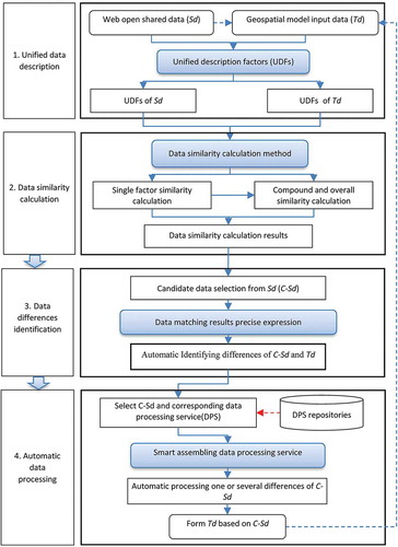
Because the description of $Sd$is quite different from that of $Td$, first the Unified Description Factors(UDFs) are used to ensure that the attributes of $Sd$ and $Td$are described using the same syntax and semantic standard. This allows the similarity between $Sd$and $Td$at different levels to be calculated. The data similarity includes the single factor similarity, the compound similarity of several factors and the overall similarity for all factors. The degree of data similarity for different factors and levels may be calculated using very different methods. If there is a $Sd$whose overall similarity is equal to 1, it can be directly input into the geospatial model and the automatic data- matching task is then finished. Otherwise (in practice, in most cases), it is necessary to continue to the third step and do some further work.

In the third step, the $Sd$ closest to $Td$is first selected as the candidate. In the selection of the candidate data, the $Sd$are sorted based on their similarity values from large to small, and the $Sd$whose similarity values are greater than a designated threshold are selected as candidate data. There are also some special rules that must be considered in candidate data selection. For instance, the similarity value of the data content must be greater than 0 – that is the data content must be relevant – and the spatial and temporal topology cannot be disconnection type. Subsequently, these candidate data-matching results are precisely expressed and formalized in order to automatically identify the types and ranges of differences between the candidate data and $Td$.

Based on the matching results and according to the differences types and ranges, one or several candidate data and corresponding data processing service(s) are selected; these are then assembled to form a data-processing service chain. It should be noted that a DPS needs to be developed in advance or else obtained from existing open DPS repositories which comply with the Web Processing Service (WPS) standard proposed by the OGC (Open Geospatial Consortium). Using the data-processing service chain, the candidate data differences can be automatically handled one by one so that target data that fully meet the requirements of the geospatial model can be produced.

4. Key issues and challenges

In the general automatic data-matching general framework described above, there exist four key issues that include the need for unified description factors, the data similarity calculation method, the precise expression of the data-matching results, and the smart assembly of the data-processing services. Unless these are properly handled, fully automatic data matching is difficult to achieve. To a large extent, these factors decide the degree, precision and efficiency of the data matching.

4.1. Unified description factors

Having a unified data description is a precondition of the similarity calculation for $Sd$ and $Td$. Since the existing open data description standards are quite different from those of geospatial models, and these standards include different factors which may vary in terms of syntax and semantics, the key to having a unified data description is to use unified description factors (UDFs) to re-describe $Sd$ and $Td$ so that the homogeneity of the data descriptions can be ensured.

The main existing geospatial data description metadata standards include the Content Standard for Digital Geospatial Metadata (FGDC 1998); ISO 19,115: Geographic information-Metadata (ISO 2003); and DIF: Directory Interchange Format (NASA 2018). The input data declarations for geospatial models are usually included in interface specifications; these include WPS: Web Processing Service Specification(OGC 2007); OpenMI: Open Modelling Interface Standard(OGC 2014); GeoMSI: Geospatial Model Service Interface(Feng et al. 2011); and UDX: Universal Data eXchange model(Yue et al. 2015, 2016). Although several of the descriptive items – such as title and abstract – in the metadata standards and model interface specifications are the same, they have different emphases. The former pay more attention to spatial and temporal scope, as well as the spatial reference system, data quality and the dissemination of information, whereas, WPS, OpenMI and GeoMSI focus more on the data type, structure, format, and encoding, with UDX containing the two basic elements Node and Kernel that describe the structure and type of the model data hierarchy (Yue et al. 2016). In addition, neither the metadata standards nor the interface specifications describe the morphological and semantic features of geospatial data completely or accurately.

Therefore, by integrating elements of the metadata standards and model interface specifications, we have proposed the Unified Description Factors (Zhu et al. 2017a). This paper goes further and, based on the the requirements of fully automatic matching of data for geospatial models, expands and optimizes the existing UDFs, as shown in Table 1. The new UDFs include not only the intrinsic features of data content, and spatial and temporal coverage and precision, but also the morphological features of data type, format or structure, and the semantic features of attribute fields, units, and classification system.

Table 1. Unified description factors (UDFs).

Data feature type	UDF class	UDF name			UDF type	Maximum occurrence (constraint)
Data intrinsic features	Data content	Title			String	1(M)
		Keywords			String	N(O)
		Abstract			String	1(O)
		Topic category			Enumeration	N(O)
	Spatial coverage	Location description			String	1(C)
		Coordinates 1(C)	West longitude		Numeric	1(M)
			East longitude		Numeric	1(M)
			South latitude		Numeric	1(M)
			North latitude		Numeric	1(M)
	Temporal coverage	Time description			String	1(C)
		Data date 1(C)	Start date		Date	1(M)
			End date		Date	1(M)
	Spatial precision	Scale			Numeric	1(C)
		Resolution			Numeric	1(C)
		Spatial granularity			Enumeration	1(O)
		Vertical stratified depth			Numeric	1(O)
	Temporal precision	Temporal granularity			Enumeration	1(M)
Data morphological features	Spatial datum	Projection reference system			Enumeration	1(O)
		Coordinate reference system			Enumeration	1(O)
		Elevation reference system			Enumeration	1(O)
	Data organization	Data type			Enumeration	1(M)
		Data format 1(C)		Format name	Enumeration	1(M)
				Format version	Numeric	1(O)
		Data structure			GML	1(C)
Data semantic features	Data semantic	Attribute fields 1(O)		Field name	String	1(M)
				Field unit	Enumeration	1(O)
				Classification system	String	1(O)
		Coordinate unit			Enumeration	1(O)
		Resolution unit			Enumeration	1(O)
		Depth unit			Enumeration	1(O)

In Table 1, GML is the Geography Markup Language, which is an XML (eXtensible Markup Language) encoding for the transport and storage of geographic information (OGC 2002). The constraint M, which indicates a factor or element to be documented, is mandatory; O is optional and represents a factor or element that may either be documented or not be documented; C is conditional and expresses a choice between two or more factors, with at least one factor being mandatory, meaning that it must be documented. A conditional factor must have one or more counterparts: for example, the counterpart of Location description is Coordinates; the counterpart of Time description is Data date; the counterpart of Scale is Resolution; and the counterpart of Data format is Data structure.

An advantage of UDFs is that they eliminate the syntactical and semantic differences between existing data description standards, and build a bridge between open online geospatial data and the input data requirements of geospatial models. They thus pave the way for the subsequent data similarity calculation. However, there are still some challenges related to the use of UDFs, including the following. (1) The core idea of UDFs is that each factor should be unambiguous and there is a consensus regarding its definition and semantics. This means that, in the future, it will be necessary to precisely define UDFs using existing ontology. (2) UDFs should be dynamically extendable according to the requirements of fully automatic data matching; however, there must be a guarantee that revised or added factors do no conflict with the original factors; (3) A disadvantage of using UDFs is the need to transform existing geospatial data and model standards to UDFs, and these transformation are complex and workload-intensive because the existing standards are very different from each other. Therefore, how to establish the mapping between these standards and the UDFs so that the unified data descriptions can be efficiently implemented is a major challenge in practical applications, and will be one of important issues considered in our future research.

4.2. Data similarity calculation method

Data similarity is the basis of automatic data matching for geospatial models. It decides whether $Sd$is directly input into the geospatial model, or discarded as useless data, or taken as candidate data to be further processed. Therefore, data similarity calculation methods are very important and can seriously affect the accuracy and efficiency of the similarity calculation.

Generally speaking, there are three types of data similarity: single factor similarity, compound similarity and overall similarity. Compound and overall similarity are usually calculated by using the analytic hierarchy process (AHP) (Zhu et al. 2017a). The single factor similarity calculation methods can be very different and complex because each individual factor has various types and characteristics. In general, the single similarity calculation methods can be divided into two types: quantitative calculation methods, and qualitative comparison measures. The former includes semantic, spatial, and temporal similarity calculations whereas the latter is based on a keyword comparison that determines whether the $Sd$and $Td$factor value is the same, totally different or partially consistent. In the case of partial consistency, the similarity needs to be further divided into several different levels depending on the degree of consistency. This is done using expert field expert knowledge.

Semantic similarity is commonly expressed as the semantic distance – the methods of calculating this again include two main types of algorithm. The first type of algorithm is the edit distance: i.e. the Levenshtein distance or one of its variant algorithms (Petroni and Serva 2010; Wichmanna et al. 2010). The second type of algorithm includes th taxonomy tree or the network path length. These are based on existing ontologies or dictionaries such as Wordnet or Hownet (Wu and Palmer 1994; Lee, Huh, and McNiel 2008; Liu, Bao, and Xu 2012). Within these ontologies or dictionaries, there is only one path for any two concept nodes, and the path length is just the semantic distance between them: the larger the semantic distance, and the smaller the similarity.

Spatial similarity calculation covers spatial topology as well as the the calculation of spatial distance or area proportion. Spatial topology calculations mainly make use of the region connection calculus model (RCC), the 4-intersection model, or the 9-intersection model as well as improved versions of this, such as the Voronoi map-based V9I model (Chen et al. 2000). In general, the similarity is given as 1 when the spatial topology relationship is equal or containing; the similarity is set to 0 when the spatial topology relationship is disjoint or adjacent. The similarity is greater than 0 and less than 1 if the spatial topology relationship is inside or intersection, and its exact value is determined by the spatial distance (Euclidean distance) or area proportion (Mesquitaa et al. 2017).

As with spatial similarity, temporal similarity calculations also include temporal topology and distance calculations. The biggest difference between temporal topology and spatial topology is that the former needs to consider the time direction (before or after) (Zhu et al. 2017a). Generally, it is assumed that the new data are better than the old. Therefore, when the temporal topology is disjoint or adjacent but the time of $Sd$is later than $Td$, the similarity is not set to 0. The key to temporal distance calculation is to unify the time granularity of $Sd$and $Td$. For example, the temporal granularity of $Td$is day, and the counterpart of $Sd$should be day rather than year or hour; otherwise, the temporal granularity of $Sd$must be transformed to day.

In summary, three types of data similarity calculation method have been widely studied: (1) quantitative calculation methods for single factor similarity, (2) qualitative comparison methods for single factor similarity, and (3) use of the AHP for compound and overall similarity. In terms of the quantitative calculation algorithms, finding algorithms that can adapt to features of individual factors and find a good balance between accuracy and efficiency is still difficult challenge and a topic for future research. In contrast, the second type – the qualitative comparison methods – do not need complex algorithms, but require consistent or interchangeable semantic descriptions of comparative items. In the case of the compound or overall data similarity, since these are usually calculated using the AHP, it is very important that the weights of all participating factors are reasonable and reflect their contributions to the compound or overall data similarity. In addition to the traditional expert scoring method, the use of the in-depth learning-based method for the weight assignment will be an important research direction in the future.

4.3. Precise expression of data-matching results

In the case of the incomplete matching candidate data, i.e data for which the similarity is greater than 0 and less than 1, further automatic processing based on series of web data processing services (DPSs) is needed. However, several questions remain including how do we know which DPSs to use, which data should be processed, and how should they be processed? In order to answer these questions, the data-matching results must be precisely and semantically expressed to record the differences between $Sd$and $Td$.

Existing research mainly focuses on the optimization of the ranking of search results obtained from well-known online search engines, such as Google, Baidu, etc. as well as various professional network searches. Many sorting algorithms exist, including word frequency statistics, word position weighted sum, link analysis ranking, attribute characteristics correlation degree sorting, and the latest knowledge graph method etc. (Jindal, Bawa, and Batra 2014; Fionda, Gutierrez, and Pirrò 2016; Goel et al. 2019). These sorting methods can generally reflect the matching degree between retrieval results and user requirements, but they cannot precisely record the differences between retrieval results and target needs. Therefore, it is difficult to achieve the proposed automatic processing of candidate data in this way.

The precise expression of data matching results includes two parts: the quantitative similarity values and semantic matching sets. The second part comprises the matching relations and extent, which precisely record the differences in syntax and semantics between $Sd$and $Td$. The form for expressing the matching results is shown as Equation (2). In practice, matching results are expressed by the XML (eXtensible Markup Language)-based RDF (Resource Description Framework), which is a machine-understandable language.

(2) $MR=\{{\text{S}}_t,D_t\{\underset{i=1}{\overset{n}{S_i}},\underset{i=1}{\overset{n}{R_i}},\underset{i=1}{\overset{n}{E_i}}\left\}\right\}$(2)

where $MR$is the expression for the matching results,$S_t$is the overall similarity value, $D_t$ is the overall semantic matching set, $S_i$ is the similarity value of the $i^{th}$ factor, $R_i$ is the matching relation for the $i^{th}$ factor, and $E_i$ is the matching extent of the $i^{th}$ factor. The total number of factor is $n$.

The quantitative similarity value is a control factor: only when it is greater than 0 and less than 1 are the semantic matching sets needed. In the semantic matching sets, the matching relation can semantically reflect the difference type, which is used to guide the DPS selection through the linkage between the matching relation and the DPS (see Table 2). The matching extent precisely expresses the difference size to assist in the choice of the candidate data and their processing range. For example, if the spatial topology relation is intersection, this indicates that the spatial clip processing service should be used to extract the ‘intersection’ part of the data from $Sd$whereas the intersection boundaries can be precisely defined by the matching extent based on GeoJSON (a format used to encode a variety of geographic data structures).

Table 2. Links between matching relations and DPS.

Matching relation type	Matching relation instance(Sd relative to Td)	Data processing service
Data content semantic relation	Same	/
	Hypernym	ContentExtract
	Hyponym	ContentFusion
	SiblingConcept	/
	Different
Spatial topology relation	Same	/
	Intersect	SpatialClipping, SpatialMerge
	Contain	SpatialClipping
	Within	SpatialClipping, SpatialMerge
	Touch	/
	Disjoint	/
Temporal topology relation	Same	/
	Intersect	TemporalExtract, TemporalCombine
	Contain	TemporalExtract
	Within	TemporalExtract, TemporalCombine
	Touch	/
	Disjoint	/
Spatial precision relation	Same	/
	Higher	SpatialDownScaling
	Lower	SpatialUpScaling
Temporal granularity relation	Same	/
	Higher	TemporalDownScaling
	Lower	TemporalUpScaling
Projection reference system relation	Same	/
	Different	SpatialReprojection
Coordinate reference system relation	Same	/
	Different	SpatialCRSTransform
Elevation reference system relation	Same	/
	Different	ElevationRSTransform
Data type relation	FullSame	/
	SameMainCategory	DataCategoryTransform
	SameSubCategory
	Different
Data format relation	FullSame	/
	SameFamily	DataFormatTransform
	Different
Data structure relation	Same	/
	Different	DataStructureTransform
Attribute field name relation	Same	/
	LexicalDifferent	AttributeFieldNameModify
	Different	/
Attribute field unit relation	Same	/
	Different	AttributeFieldUnitTransform
Attribute field classification system relation	Same	/
	Different	AttributeFieldCSTransform
Coordinate unit relation	Same	/
	Different	CoordinateUnitTransform
Resolution unit relation	Same	/
	Different	ResolutionUnitTransform
Depth unit relation	Same	/
	Different	DepthUnitTransform

The application schema for the precise expression of matching results used to support the automatic data processing is shown as Figure 2.

Figure 2. the application schema of matching results precise and semantic expression.

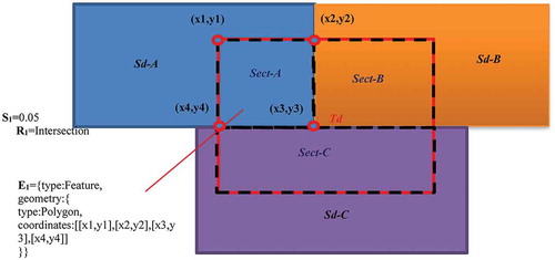
In Figure 2, it is assumed that the spatial topology relations for the geospatial model input data ($Td$, red rectangle) and its three candidate data (Sd-A, Sd-B, Sd-C) are all intersection. The intersection parts are respectively Sect-A, Sect-B and Sect-C. According to Equation (1), the matching results for each part need to precisely define the similarity value, matching relation and extent: for example, S₁ = 0.05, R1 = Intersection, and E₁ = { … coordinates: [x1, y1], [X2, y2], [X3, Y3], [x4, y4]}, express the matching results for Sd-A.

As mentioned above, the key points in the precise expression of the data-matching results are a clear matching relation and a detailed matching extent. The former decides what processing will be carried out on the candidate data while the latter determines the scope of the candidate data to be processed. Therefore, in future, two important research directions related to the precise expression of data-matching results will be (1) the need for the matching relation to be continuously expanded and clearly defined as well as have the ability to bind to specific data-processing services; and (2) the need for the matching range of the candidate data need to be recorded in more detail. This means that as many vertexes as possible should be recorded rather than just the external rectangle of the matching part.

4.4. Smart assembly data-processing services

Based on the precise expression of the data-matching results, one or several candidate data and corresponding DPS(s) will be automatically selected and smart assembled to form the specific data-processing service chain. Using the data-processing service chain, all differences between $Sd$and $Td$ can be automatically handled step by step, and data that are fully consistent with the geospatial model requirements will eventually be generated.

According to the application objectives, the online processing service should arrange and compose a series of related existing online processing services appropriate to the order of the task execution, and then process the specified input data step by step (Yue et al. 2009; Sun, Peng, and Di 2012; Chen, Zhang, and Wang 2015). For example, in order to prepare and process data for geo-analysis models, three types of data processing services based on the UDX model – the data-mapping process, data-refactoring process and visualization process services are need (Wang et al. 2018). Compared with the composition of existing online processing services, the method of assembling data-processing services proposed in this paper is more complex and intelligent because its application objectives, input data and processing range are all undefined in advance – the matching results are dynamically parsed to obtain the precise differences between $Sd$and $Td$, and, subsequently, the application objectives, input data and processing range are intelligently deduced.

The workflow for smart assembling DPSs is as follows. First, the similarity value of each candidate data is parsed from the matching result expression. If the similarity value is 1 or 0, there is no need to further parse matching relation and extent of the candidate data. Otherwise, the matching relation and extent are further parsed to guide the selection of specific DPSs and clarify their range. DPSs should have the ability of process the possible differences between $Sd$and $Td$, and especially the differences in UDFs shown in Table 1. Based on the UDFs, DPSs can be divided into the following types: data content, spatial coverage, temporal coverage, spatial precision, temporal precision, spatial datum, data organization, data semantic processing, and transformation services. In practice, each type of DPS contain a series of specific services. For examples, spatial-coverage processing services include spatial clipping, spatial merging and spatial overlay; spatial-datum transformation services include coordinate system conversion, projection transformation; etc. Taking the example of the application shown in Figure 2, the detailed procedure for the smart-assembly of DPSs is as shown in Figure 3.

Figure 3. the workflow of smart assembling DPSs to automatic processing data.

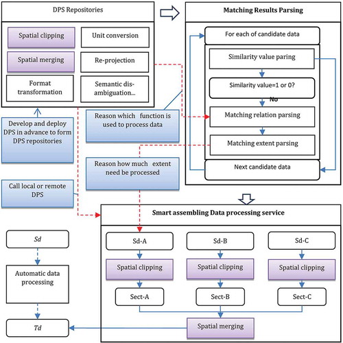
In the example shown in Figure 3, either the DPS repository needs to be developed locally in advance or open-data processing services need to be called in real time. Moreover, these DPSs must adhere to OGC WPS; otherwise, it is difficult to assemble them because of their heterogenous interfaces and semantics. Therefore, building a perfect DPS repository will be one of the key points of our future research. For DPS development, in order to improve the efficiency and shorten the cycle, it is possible to use existing geospatial data-processing open-source libraries, such as GDAL (Geospatial Data Abstraction Library) released by the Open Source Geospatial Foundation (Warmerdam 2008). It is worth noting that, in order to deal with the limitation of the simple data type used in WPS, in our approach, each DPS is firstly given the input data address from ListDiff.xml; the complex data are then downloaded and handled by data-parsing functions that are built into each DPS. When, remote calling existing open DPSs, the key is to maintain their compatibility with OGC WPS, and also maintain network accessibility and stability. DPS sharing, standardization and quality assessment will, therefore also be issues that we will consider in future research.

5. Case study

5.1. Target model and source data

Guizhou province, located in the southwest of China, is a typical karst region. The assessment and conservation of soil and water loss are of great significance to the sustainable development of Guizhou. This case study takes calculating the soil and water loss in Guizhou from 2000 to 2010 as an application that uses the revised universal soil loss equation (RUSLE) (Renard, Foster, and Weesises 1997) as the target model, and the open data in the National Earth System Scientific Data Sharing Platform of China (Geodata.CN¹) as the source data.

In the RUSLE model, the soil and water loss amount (A) is equal to the product of the rainfall erosivity factor (R), soil erodibility factor (K), slope length factor (L), slope factor (S), vegetation and management factor (C), and the soil and water conservation measure factor (P) (see Equation 3).

(3) $\mathrm{A}=R\times K\times L\times S\times C\times P$(3)

where R, the rainfall erosivity factor, reflects the potential of soil erosion caused by rainfall and the influence of climatic factors on water power: it can be calculated using Equation 4 (Wischmeier and Simth 1978).

(4) $\mathrm{R}=\sum _{\hspace{0.17em}}^{\hspace{0.17em}}1.735\times {10}^{[(1.5\times lg\frac{{p_i}^2}{p})-0.8188]}$(4)

Here P_i is the monthly rainfall (mm), and P denotes the annual rainfall (mm). In the example of the calculation of the 2000–2010 soil and water loss for Guizhou, only the automatic matching of data from Geodata.CN with the RUSLE parameter P is considered in detail to illustrate our proposed new framework. The data matching for the other RUSLE parameters is similar to that for P.

Geodata.CN was launched in 2003 and supported by the Ministry of Science and Technology of China. It is one of China’s national sciences and technology infrastructures (NSTI). It adopts a service-oriented architecture to provide one-stop data sharing and open service, and ISO19115-based metadata to describe the core characteristics of datasets and data documents to record the other features of datasets (Zhu et al. 2017a). So far, Geodata.CN holds about 150 TB of data resources covering different disciplines, such as geography, geophysics, hydrology, atmosphere, resource science, and the ecological environment (Zhu et al. 2017b).

5.2. UDFs of input parameter P of RULSE and source data

All of the mandatory factors and some of the important optional factors for RUSLE input parameter P that are shown in Table 1 are described in Table 3.

Table 3. UDFs of the RUSLE input parameter P.

Input parameter P (annual rainfall) for calculating 2000–2010 Guizhou soil and water loss amount
		Data date								Attribute fields
Title	Location description	Start date	End date	Resolution	Temporal granularity	Projection reference system	Coordinate reference system	Data type	Data format name	Field name	Field unit	Resolution unit
Guizhou 2000–2010 annual 1 km raster rainfall	Guizhou province	2000	2010	1	Annual	Albers	WGS 84	Spatial raster	Arc/Info ASCII Grid	rainfall	mm	km

In Geodata.CN, there are 100 datasets related to rainfall. These dataset descriptions are converted to UDFs taken from ISO19115-based metadata by using appropriate pre-customized mapping templates. The UDFs of some of the datasets are shown in Table 4. For these 100 relevant datasets, each single factor similarity, compound similarity and overall similarity are respectively calculated. The detailed calculation methods can be found in the reference of Zhu et al (2017a, 2017b). According to the candidate data selection rules described in section 3.2, only ‘2000–2010 China 1 km annual rainfall raster dataset’ can be selected in this case, for the other 99 datasets, either the content similarity, the spatial coverage similarity, or the temporal coverage similarity is equal to 0.

Table 4. UDFs of some of the related source data.

		Data date								Attribute fields
UDFs Name	Location description	Start date	End date	Resolution	Temporal granularity	Projection reference system	Coordinate reference system	Data type	Data format name	Field name	Field unit	Resolution unit
No.1	Title:2000–2010 China 1km annual rainfall raster dataset
UDFs value	China	2000	2010	1	Annual	Albers	WGS 84	Spatial raster	GeoTiff	rainfall	mm	km
No.2	Title: 30m resolution rainfall erosivity map of China
UDFs value	China	1981	2010	30	Annual	Albers	WGS 84	Spatial raster	ESRI Grid	rainfall erosivity	MJ•mm/(ha•h•a)	m
No.3	Title: Average rainfall distribution map of many years with 500 m resolution of China
UDFs value	China	Station setup time	1980	500	Annual	Albers	WGS 84	Spatial raster	GeoTiff	rainfall	mm	m
No.4	Title: Monthly rainfall database for Central plains economic zone in recent years
UDFs value	Central plains economic region	2000	2012	2	Monthly	Albers	Xi’an 80	Spatial raster	GeoTiff	rainfall	mm	km
…

5.3. Precise expression of matching results for RULSE input parameter P

The results of the data matching between RULSE input parameter P and the candidate data is precisely expressed by using XML, and is stored in the file named ListDiff.xml, as shown in Figure 4.

Figure 4. the XML-based precise expression of data matching result.

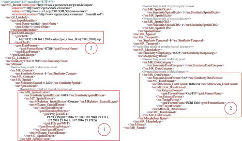
From Figure 4, it is clear that there are two differences between RULSE input parameter P and the candidate data. The first difference (marked by the red rectangle 1 in Figure 4) is the quantitative difference in spatial coverage (Guizhou versus China). The similarity value is equal to 0.018; the matching relation is ‘Contain’; the coordinates of the matching range are accurately recorded using a WKT (well-known text) polygon. The second difference (the red rectangle 2 in Figure 4) corresponds to a qualitative difference in data format: for this, the similarity value is equal to 0.65; the matching relation is ‘Different’; the source format is ‘ESRI Grid’ and the target format is ‘GeoTiff’.

5.4. Automatic data processing based on the precise expression of the matching result

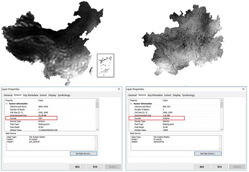
By parsing the file ListDiff.xml, the differences ‘spatial coverage’ and ‘data format’, along with their matching relations and matching range, can be automatically identified. Given the matching relations ‘spatial contain’ and ‘format different’, the corresponding data-processing services ‘spatial clipping’ and ‘format transformation’ are then selected and executed. These data-processing services were developed in advance based on OGC WPS. Moreover, the required parameters for the ‘spatial clipping’ data-processing service, i.e. the source data and the clipping coverage, are retrieved through the ‘DataLinkage’ and ‘PolygonWKT’ elements of ListDiff.xml, respectively. After the ‘spatial clipping’ data-processing service has been successfully executed, the ListDiff.xml file is simultaneously updated, with the ‘format transformation’ data-processing service being marked as the currently activated service and the ‘DataLinkage’ element value is set to the output data of the previous service. The required parameters for the ‘format transformation’ data processing service, i.e. the original and target format, are obtained from the ‘OriginalFormat’ and ‘TargetFormat’ elements of ListDiff.xml. Detailed of the workflow for automatic processing of ‘2000–2010 China 1km annual rainfall raster dataset’ based on the precise expression of the matching result, and the final data-processing result for the case study are shown as Figures 5 and 6, respectively.

Figure 5. the workflow of data automatic processing of the case study.

Figure 6. the data matching and processing result of the case study.

6. Conclusions and discussions

Automatic matching of data from existing open and shared web portals is a highly efficient and innovative framework of input data preparation for geospatial models. It is also a new paradigm that links and promotes the integrated sharing of geospatial data and models. Open and shared data can be selected as candidate data and seamlessly input into geospatial models after they have been properly processed or transformed. This framework thus not only promotes the application of geospatial models, but also greatly improves the value of open data.

It is worth noting that automatic data matching is a comprehensive activity. It includes the four steps of unified data description, data similarity calculation, data difference identification, and automatic data processing. The four key issues in the workflow are the use of unified description factors, the data similarity calculation method, the precise expression of matching results, and the smart assembly of data- processing services. These issues need to be dealt with carefully as they may affect not only the accuracy of the automatic data matching but also its efficiency.

In the future, more efforts should be made towards improving and optimizing the workflow and deal with the key issues described above. First, it is necessary to dynamically expand and unambiguously define UDFs based on ontology so that the open data and the geospatial model input data can be described in a consistent way. Moreover, in order to adapt to the requirements of different disciplines and domains of geospatial data and models, the corresponding optional and conditional UDFs factors can be adjusted or selected based on the maintenance of the consistency of the mandatory factors. At the same time, there is an urgent need to develop new tools to efficiently transform the descriptions of existing open data and geospatial model input data to UDFs. Secondly, the development of more accurate similarity calculation methods that accord with the characteristics of each UDF and that use state-of-the-art deep learning and knowledge graphs should be a focus of future research. Meanwhile, once the source data expands to include all of the geospatial data that is available online, the computational workload related to the data similarity calculations will increase dramatically. Therefore, improving the efficiency of the data similarity calculation will be another important research topic – its solution will depend not only on cloud computing technology, but also on a reasonable data-selection strategy. Thirdly, the precise expression of the data-matching result is the basis of smart assembly data-processing services. Therefore, how to automatically adjust and optimize the order of data-processing services based on the precise expression of the data-matching results, and also dealing with data-processing exceptions, will be the focus of our subsequent research. Finally, automatic data-processing depends on existing DPSs, which means that lots of DPSs need to be developed and shared in advance. Meanwhile, it is worth noting that some data differences are very difficult to process online – or maybe cannot be processed at all. This includes, for example, the conversion of raster data to vector data. Therefore, such data processing services should be excluded when generating the data processing services chain.

The big data era and the fourth research paradigm, i.e. data-intensive scientific research, require the use of massive scientific data through mining analysis, simulation and prediction methods to discover and look for hidden laws and issues in scientific research (Hey and Trefethen 2005). It is very important to urgently develop the integrated sharing of geospatial data and models – e-Geoscience – to facilitate their usage (Zhu et al. 2016). An automatic data-matching framework is the indispensable foundation for bridging the gap between geospatial data and models, and for supporting the development of the fourth research paradigm.

Acknowledgements

The authors would like to thank for the editor in chief and the anonymous reviewers for their very helpful suggestions that improved the article.

Disclosure statement

No potential conflict of interest was reported by the authors.

Additional information

Funding

This work was supported by the Natural Science Foundation of China [Nos. 41771430 and 41631177], the National Special Program on Basic Works for Science and Technology of China [No. 2013FY110900], and the Strategic Priority Research Program of the Chinese Academy of Sciences [No. XDA23100100].

Notes

1. National Earth System Scientific Data Sharing Platform of China: http://www.geodata.cn.

References

- Arnold, J. G., and N. Fohrer. 2005. “SWAT2000: Current Capabilities and Research Opportunities in Applied Watershed Modelling.” Hydrological Processes 19 (3): 563–572. doi:10.1002/hyp.5611.
- Aydinoğlu, A. Ç., and A. Kara. 2017. “Modelling and Publishing Geographic Data with Model-driven and Linked Data Approaches: Case Study of Administrative Units in Turkey.” Journal of Spatial Science 4: 1–21. doi:10.1080/14498596.2017.1368420.
- Bai, Y., and L. Di. 2012. “Review of Geospatial Data Systems’ Support of Global Change Studies.” British Journal of Environment & Climate Change 2 (4): 421–436. doi:10.9734/BJECC/2012/2726.
- Bernard, L., I. Kanellopoulos, A. Annoni, and P. Smits. 2005. “The European Geoportal-One Step Towards the Establishment of A European Spatial Data Infrastructure.” Computers, Environment and Urban Systems 29: 15–31. doi:10.1016/j.compenvurbsys.2004.05.009.
- Bone, C., A. Ager, K. Bunzel, and L. Tierney. 2014. “A Geospatial Search Engine for Discovering Multi-format Geospatial Data across the Web.” International Journal of Digital Earth 9 (1): 47–62. doi:10.1080/17538947.2014.966164.
- Chen, J., C. Li, Z. Li, and C. M. Gold. 2000. “Improving 9-intersection Model by Replacing the Complement with Voronoi Region.” Geo-spatial Information Science 3 (1): 1–10. doi:10.1007/BF02826800.
- Chen, N., X. Zhang, and C. Wang. 2015. “Integrated Open Geospatial Web Service Enabled Cyber-Physical Information Infrastructure for Precision Agriculture Monitoring.” Computers and Electronics in Agriculture 111: 78–91. doi:10.1016/j.compag.2014.12.009.
- Dile, Y. T., P. Daggupati, C. George, R. Srinivasan, and J. Arnold. 2016. “Introducing A New Open Source GIS User Interface for the SWAT Model.” Environmental Modelling & Software 85: 129–138. doi:10.1016/j.envsoft.2016.08.004.
- Dowman, I., and H. I. Reuter. 2017. “Global Geospatial Data from Earth Observation: Status and Issues.” International Journal of Digital Earth 10 (4): 328–341. doi:10.1080/17538947.2016.1227379.
- Elliott, J., C. Müller, D. Deryng, J. Chryssanthacopoulos, K. J. Boote, M. Büchner, I. Foster, et al. 2015. “The Global Gridded Crop Model Intercomparison: Data and Modelling Protocols for Phase 1 (v1.0).” Geoscientific Model Development 8 :261–277. doi:10.5194/gmd-8-261-2015.
- Erol, A., Ö. Koskan, and M. A. Basaran. 2015. “Socioeconomic Modifications of the Universal Soil Loss Equation.” Solid Earth 6: 1025–1035. doi:10.5194/se-6-1025-2015.
- Eyring, V., S. Bony, G. A. Meehl, C. A. Senior, B. Stevens, R. J. Stouffer, and K. E. Taylor. 2016. “Overview of the Coupled Model Intercomparison Project Phase 6 (CMIP6) Experimental Design and Organization.” Geoscientific Model Development 9: 1937–1958. doi:10.5194/gmd-9-1937-2016.
- Feng, M., S. Liu, N. H. Euliss, C. Young, and D. M. Mushet. 2011. “Prototyping an Online Wetland Ecosystem Services Model Using Open Model Sharing Standards.” Environmental Modelling & Software 26: 458–468. doi:10.1016/j.envsoft.2010.10.008.
- FGDC (Federal Geographic Data Committee). 1998. FGDC-STD-001-1998:Content Standard for Digital Geospatial Metadata. Washington, D.C: Federal Geographic Data Committee.
- Fionda, V., C. Gutierrez, and G. Pirrò. 2016. “Building Knowledge Maps of Web Graphs.” Artificial Intelligence 239: 143–167. doi:10.1016/j.artint.2016.07.003.
- Foley, J. A., I. C. Prentice, N. Ramankutty, S. Levis, and D. Pollard. 1996. “An Integrated Biosphere Model of Land Surface Processes, Terrestrial Carbon Balance, and Vegetation Dynamics.” Global Biogeochemical Cycles 10 (4): 603–628. doi:10.1029/96GB02692.
- Goel, S., R. Kumar, M. Kumar, and V. Chopra. 2019. “An Efficient Page Ranking Approach Based on Vector Norms Using sNorm (p) Algorithm.” Information Processing and Management 56: 1053–1066. doi:10.1016/j.ipm.2019.02.004.
- Goodchild, M. F., P. Fu, and P. Rich. 2007. “Sharing Geographic Information: An Assessment of the Geospatial One-Stop.” Annals of the Association of American Geographers 97 (2): 250–266. doi:10.1111/j.1467-8306.2007.00534.x.
- Gregersen, J. B., P. J. A. Gijsbers, and S. J. P. Westen. 2007. “OpenMI: Open Modelling Interface.” Journal of Hydroinformatics 9 (3): 175–191. doi:10.2166/hydro.2007.023.
- Hey, T., S. Tansley, and K. Tolle. 2009. The Fourth Paradigm: Data Intensive Scientific Discovery. Redmond, Washington: Microsoft Corporation.
- Hey, T., and A. E. Trefethen. 2005. “Cyberinfrastructure for e-Science.” Science 308: 817–821. doi:10.1126/science.1110410.
- Hu, S., and L. Bian. 2009. “Interoperability of Functions in Environmental Models-A Case Study in Hydrological Modeling.” International Journal of Geographical Information Science 23 (5): 657–681. doi:10.1080/13658810902733674.
- Hudak, P. F. 2014. “Inundation Patterns and Plant Growth in Constructed Wetland Characterized by Dynamic Water Budget Model.” Environmental Earth Sciences 72 (6): 1821–1826. doi:10.1007/s12665-014-3091-2.
- Hurrell, J. W., M. M. Holland, P. R. Gent, S. Ghan, J. E. Kay, P. J. Kushner, J. F. Lamarque, et al. 2013. “The Community Earth System Model: A Framework for Collaborative Research.” Bulletin of the American Meteorological Society 94 (9): 1339–1360. doi:10.1175/BamS-d-12-00121.1.
- ISO (the International Organization for Standardization). 2003. ISO 19115: 2003(E) Geographic information-Metadata.
- Jindal, V., S. Bawa, and S. Batra. 2014. “A Review of Ranking Approaches for Semantic Search on Web.” Information Processing and Management 50: 416–425. doi:10.1016/j.ipm.2013.10.004.
- Lee, S., S. Y. Huh, and R. D. McNiel. 2008. “Automatic Generation of Concept Hierarchies Using WordNet.” Expert Systems with Applications 35: 1132–1144. doi:10.1016/j.eswa.2007.08.042.
- Liu, H., H. Bao, and D. Xu. 2012. “Concept Vector for Semantic Similarity and Relatedness Based on WordNet Structure.” The Journal of Systems and Software 85: 370–381. doi:10.1016/j.jss.2011.08.029.
- Mesquitaa, D. P. P., J. P. P. Gomes, A. H. S. Junior, and J. S. Nobre. 2017. “Euclidean Distance Estimation in Incomplete Datasets.” Neurocomputing 248: 11–18. doi:10.1016/j.neucom.2016.12.081.
- NASA (National Aeronautics and Space Administration). 2018. “Directory Interchange Format (DIF) Writer’s Guide.” Global Change Master Directory. https://gcmd.nasa.gov/add/difguide
- Nativi, S., P. Mazzetti, and G. N. Geller. 2013. “Environmental Model Access and Interoperability: The GEO Model Web Initiative.” Environmental Modelling & Software 39 (1): 214–228. doi:10.1016/j.envsoft.2012.03.007.
- OGC (Open GIS Consortium). 2002. “OpenGIS Geography Markup Language (GML) Implementation Specification, version 2.1.2.”.
- OGC (Open GIS Consortium). 2007. “OpenGIS Web Processing Service, version 1.0.0”.
- OGC (Open GIS Consortium). 2014. “Open Modelling Interface Interface Standard, Version 2.0.” http://www.opengis.net/doc/IS/openmi/2.0
- Petroni, F., and M. Serva. 2010. “Measures of Lexical Distance between Languages.” Physica A Statistical Mechanics & Its Applications 389: 2280–2283. doi:10.1016/j.physa.2010.02.004.
- Renard, K. G., G. R. Foster, and G. A. Weesises. 1997. Predicting Soil Erosion by Water: A Guide to Conservation Planning with the Revised Universal Soil Loss Equation (RUSLE). Washington DC: United States Department of Agriculture.
- Risse, L. M., M. A. Nearing, A. D. Nicks, and J. M. Laflen. 1993. “Error Assessment in the Universal Soil Loss Equation.” Soil Science Society of America Journal 57 (3): 825–833. doi:10.2136/sssaj1993.03615995005700030032x.
- Sun, Z., Y. Peng, and L. Di. 2012. “GeoPWTManager: A Task-Oriented Web Geoprocessing System.” Computers & Geosciences 47: 34–45. doi:10.1016/j.cageo.2011.11.031.
- Wang, J., M. Chen, G. Lü, S. Yue, K. Chen, and Y. Wen. 2018. “A Study on Data Processing Services for the Operation of Geo-analysis Models in the Open Web Environment.” Earth and Space Science 5: 844–862. doi:10.1029/2018EA000459.
- Warmerdam, F. 2008. “The Geospatial Data Abstraction Library.” In Open Source Approaches in Spatial Data Handling, edited by G. B. Hall and M. G. Leahy, 87–104. Berlin, Heidelberg: Springer.
- Wen, Y., M. Chen, G. Lu, H. Lin, L. He, and S. Yue. 2013. “Prototyping an Open Environment for Sharing Geographical Analysis Models on Cloud Computing Platform.” International Journal of Digital Earth 6 (4): 356–382. doi:10.1080/17538947.2012.716861.
- Wichmanna, S., E. W. Holman, D. Bakker, and C. H. Brown. 2010. “Evaluating Linguistic Distance Measures.” Physica A Statistical Mechanics & Its Applications 389: 3632–3639. doi:10.1016/j.physa.2010.05.011.
- Wischmeier, W. H., and D. D. Simth. 1978. Predicting Rainfall Erosion Losses-A Guide to Conservation Planning. Washington, DC: United States Department of Agriculture.
- Wu, Z., and M. Palmer. 1994. “Verb Semantics and Lexical Selection.” Paper presented at the 32nd annual meeting of the association for computational linguistics. Las Cruces, New Mexico, Stroudsburg, June 27–30.
- Xu, C., and C. Yang. 2014. “Introduction to Big Geospatial Data Research.” Annals of GIS 20 (4): 227–232. doi:10.1080/19475683.2014.938775.
- Xu, G. H. 2007. “Open Access to Scientific Data: Promoting Science and Innovation.” Data Science Journal 6: OD21–OD25. doi:10.2481/dsj.6.OD21.
- Yue, P., L. Di, W. Yang, G. Yu, P. Zhao, and J. Gong. 2009. “Semantic Web Services‐based Process Planning for Earth Science Applications.” International Journal of Geographical Information Science 23 (9): 1139–1163. doi:10.1080/13658810802032680.
- Yue, S., M. Chen, Y. Wen, and G. Lu. 2016. “Service-oriented Model-encapsulation Strategy for Sharing and Integrating Heterogeneous Geo-analysis Models in an Open Web Environment.” ISPRS Journal of Photogrammetry and Remote Sensing 114: 258–273. doi:10.1016/j.isprsjprs.2015.11.002.
- Yue, S., Y. Wen, M. Chen, G. Lu, D. Hu, and F. Zhang. 2015. “A Data Description Model for Reusing, Sharing and Integrating Geo-analysis Models.” Environmental Earth Sciences 74 (10): 7081–7099. doi:10.1007/s12665-015-4270-5.
- Zhang, G., and A.-X. Zhu. 2018. “The Representativeness and Spatial Bias of Volunteered Geographic Information: A Review.” Annals of GIS 24 (3): 1–12. doi:10.1080/19475683.2018.1501607.
- Zhu, A.-X., G. Zhang, W. Wang, W. Xiao, Z. P. Huang, G. S. Dunzhu, G. Ren, et al. 2015. “A Citizen Data-based Approach to Predictive Mapping of Spatial Variation of Natural Phenomena.” International Journal of Geographical Information Science 29 (10): 1864–1886. doi:10.1080/13658816.2015.1058387.
- Zhu, Y., P. Pan, S. Fang, L. Xu, J. Song, J. Zhang, and M. Feng. 2016. “The Development and Application of e-Geoscience in China.” Information Systems Frontiers 18 (6): 1217–1231. doi:10.1007/s10796-015-9571-4.
- Zhu, Y., A.-X. Zhu, M. Feng, J. Song, H. Zhao, J. Yang, Q. Zhang, K. Sun, J. Zhang, and L. Yao. 2017a. “A Similarity-based Automatic Data Recommendation Approach for Geographic Models.” International Journal of Geographical Information Science 31 (7): 1403–1424. doi:10.1080/13658816.2017.1300805.
- Zhu, Y., A.-X. Zhu, J. Song, J. Yang, M. Feng, K. Sun, J. Zhang, Z. Hou, and H. Zhao. 2017b. “Multidimensional and Quantitative Interlinking Approach for Linked Geospatial Data.” International Journal of Digital Earth 10 (9): 1–21. doi:10.1080/17538947.2016.1266041.