Fuzzy inference approach in traffic congestion detection

ABSTRACT

One of the major tasks within the concept of an intelligent transportation system is the immediate indication of traffic breakdowns. A conventional approach evaluates a traffic condition by classifying (1) traffic volume and (2) vehicles average speed. This mathematical approach is acceptable and leads to good results as long as the analyzed data correctly represents the observed situation. However, both traffic situations and behaviour of individual drivers cannot be foreseen. In such circumstances, ‘crisp’ computational models cannot deal effectively with accompanied ambiguities and uncertainties. An alternative approach is to apply fuzzy logic systems, which enable knowledge-based analysis for effective and efficient traffic congestion detection. In this paper, traffic flow and density are inputs for the proposed fuzzy inference model and the output comes in form of detected levels of congestion (ranging from ‘congestion free’ to ‘extreme congestions’ conditions). The results show that fuzzy logic inference model for congestion detection might be highly suitable for transportation planning, management and security assessment.

KEYWORDS:

• Traffic flow theory
• traffic
• congestion
• fuzzy logic
• fuzzy inference model

Introduction

Traffic congestion is one of the major issues affecting big cities throughout the world. People seem to accept some levels of delay; however, they often face many negative impacts that traffic congestion evokes (e.g. impede mobility, increase in fuel waste, loss of time, etc.). Even though traffic congestion might be inevitable, there are ways to cope with it and slow the rate at which it intensifies. Several procedures could do that effectively, especially if used in concert. These procedures primarily refer to either building high occupancy tool and/or vehicle lanes, reacting more rapidly on the traffic-blocking accidents and incidents, extending existing or building new transportation infrastructure, etc. These actions, however, relieve the phenomena to a certain level, and, most probably, only for a limited period of time. The question is how to implement traffic guidance and control using already available road resources even more effectively?

The concept of Intelligent Transportation Systems (ITS) emerged in early nineties (Wardrop 1952) aiming to improve efficiency of surface transportation systems and solving transportation problems through modern information and communication technologies. ITS is implemented to fulfil increasing traffic demand and facilitate efficient utilization of transport infrastructure. In other words, its main role was and still is to improve the efficiency of the existing transportation system. Currently, transportation systems aim to increase the use of alternative transportation and improve traffic flow through variety of measures such as route guidance systems, traffic signal improvements, incident management and traffic flow prediction. All these measures have two things in common; to understand the nature of traffic at the specific location and control its growth. To do so, each of these measures relies mostly on traditional mathematical methods (e.g. statistical regression) and is usually unable to fully address the complexity of a road traffic characteristics and relationships. Additionally, the process of participating in a traffic flow is heavily based on the behavioural aspects associated with human drivers. As most of the traffic related decisions take place under imprecision, uncertainty and partial truth, it is immensely important and necessary to include the human factor into the modelling equations. This, additionally, leads to a severe increase in computation complexity and execution time. Therefore, we aim to bring forward a measure of congestion, which involves uncertainty (coming from impression in measurements), the traveller’s perception of acceptability, variations in data and the analyst’s uncertainty about causal relations. We approach real-life traffic congestion detection by quantifying it with subjective knowledge (linguistic information) rather than applying traditional analytical techniques. We do so because our intention is to investigate whether a knowledge-based approach could be adopted in traffic congestion detection and driver behaviour modelling. The proposed model is based on fuzzy logic theory and capable of dealing with ambiguities and uncertainties. It consist of two input variables that explain the nature of traffic congestion and one output variable, which can be used to indicate levels (severity) of detected congestion. Due to the proposed number of inputs and the number of generated fuzzy rules, the computation time and complexity is within an acceptable time frame. In addition, the proposed approach not only facilitates the understanding and analysis of congestions, but also shows efficient performance and effective traffic congestion detection possibilities with extremely high noise tolerance.

Concepts of stream parameters in traffic congestion detection

Traffic flow theory dates back to the early fifties when Wardrop (1952) described traffic flows using mathematical and statistical ideas. Traffic flow theory studies the interactions between travellers (pedestrians, cyclists, drivers and their vehicles) and infrastructure (highways, signage and traffic control devices). It aims in understanding and developing an optimal transport network with efficient movement of traffic and minimal traffic congestion (Wardrop 1952). It is considered that efficient movement of traffic is achieved through the following goals: keep traffic flowing, slow down traffic before known congestion areas and reduce risk of accidents (Krause, von Altrock, and Pozybill 1996). For this cause, the scientific field of traffic engineering defines three main properties of the traffic stream (Immers and Logghe 2008), including density, flow and mean speed. These parameters are commonly known as macroscopic traffic variables (vehicles are not seen as separate entities) and can be calculated for every location, at any point of time and for every measurement interval.

(1) $\mathrm{q}={\mathrm{k}}^{\mathrm{x}}\mathrm{u}$(1)

with flow – the number of vehicles per unit of time (q), density – the number of vehicles per unit of space (k) and mean speed – quotient of the flow rate and the density (u). Because this relation irrevocably links flow rate, density and mean speed, it is often called the fundamental relation of traffic flow theory. Additionally, knowing two of these parameters immediately leads to the remaining third. In practice, needful data for calculating these parameters is captured mostly using traffic detectors and video cameras.

Knowing these parameters has a significant role in detecting traffic congestion. The question is what is meant by traffic congestion and how it can be categorized? In which way these parameters can be set to measure and/or detect congestions? According to Aftabuzzaman (2007), traffic congestion should be seen and categorized as demand–capacity related congestion, delay-travel time and cost-related congestion.

• Demand–capacity congestion is a ratio between supply and demand or relative quality of traffic flow ratio between ideal conditions and existing conditions (Rosenbloom 1978). An imbalance between traffic flow and capacity that causes increased travel time, cost and modification of behaviour (Miller and Li 1994). It is a situation when traffic is moving at speeds below the designed capacity of a roadway (Downs 2004).

• Delay travel time congestion is travel time or delay in excess of that normally incurred under light or free-flow travel conditions (Lomax et al. 1997). It defines a condition of traffic delay (when the flow of traffic is slowed below reasonable speeds) because the number of vehicles trying to use the road exceeds the traffic network capacity to handle them (Weisbrod, Vary, and Treyz 2001). Another definition suggests a presence of delays along a physical pathway due to presence of other users (Kockelman 2004).

• Cost-related congestion refers to the incremental costs resulting from interference among road users (VTPI 2005).

Many researchers from different fields have argued upon how to measure congestion. Lomax et al. (1997) imply that an ideal congestion measure would have clarity and simplicity (understandable, unambiguous and credible). That includes a descriptive and predictive ability (ability to describe existing conditions and predict changes) and statistical analysis capability (ability to apply statistical techniques to provide a reasonable portrayal of congestion and replicability of result with a minimum of data collection requirements). Additionally, it includes general applicability to various modes, facilities and time periods.

One of the most commonly used traffic congestion measures is the level of service (LOS) represented as a grading system using one of six letters A– F where LOS–A denotes the best, while LOS–F the worst traffic conditions (May 1990). Schrank and Lomax (1997) developed a Roadway Congestion Index (RCI) as a measure of area wide severity of congestion. The daily vehicle per mile (or km) of the area is weighted by the type of the road and compared with the total expected vehicles per mile in the area under congested conditions (as well weighted by the road type). If this index has values equal or higher than 1, it indicates an undesirable area-wide congestion level. Lomax et al. (1997) developed this Relative delay rate (RDR) as a measure of flow quality relative in relation to actual and acceptable travel time. D’Este, Zito, and Taylor (1999) and Taylor (1992) developed similar measure, called Congestion Index (CI), where flow quality is measured in relation to actual and ideal (free flow) travel time.

Nonetheless, one has to keep in mind that both traffic observations and measurements are approximate. Therefore, any measure of congestion has to be associated with uncertainty regarding the accuracy of its representation of the real conditions. Real world conditions change depending on the roadway section and traffic participant’s experience and familiarity with the area. Stepwise approaches, such as LOS, can lead to a wrong impression that the measure is very well defined. However, a small change in the input can sometimes significantly change the outputs. Since congestion is seen as a vague concept, one should include combination of conditions in order to model the ‘traffic participants feeling’ into classifications like ‘acceptable’ or ‘good’. Hence, the process of determining the degree of congestion is fuzzy. It has to involve imprecise quantities and subjective notion of acceptability, as well as judgement in the calculation and interpretation of the results.

Fuzzy logic theory in transportation and traffic

Traditional analytical techniques have often found to be non-effective when dealing with problems in which the dependencies between variables are too complex or vaguely defined. Moreover, real-life situations such as traffic are frequently hard to quantify using ‘classical’ mathematical techniques. This is mostly because subjectivity judgement is present in many traffic phenomena, such as route choice, drivers’ perception, established LOS, defining criteria for alternative routing, etc. Since existing crisp–computational models for solving complex traffic and transportation engineering problems cannot deal effectively with the transport decision-makers’ ambiguities, uncertainties and vagueness, we approach to these problems by using different fuzzy set theory techniques.

Fuzzy logic system can uniformly approximate any real continuous nonlinear function to an arbitrary degree of accuracy (Mendel 1995). Terms as ambiguity, uncertainty and vagueness are used to describe traffic related events and traffic itself. Zadeh (1973) shows that vague logical statements enable the formation of algorithms that uses vague data to derive vague inferences. Pappis and Mamdani (1977) are among the first ones to solve a practical traffic and transportation problem using fuzzy logic. Nakatsuyama, Nagahashi, and Nishizuka (1984), Sugeno and Nishida (1985), Sasaki and Akiyama (1986, 1987, 1988) solve complex traffic and transportation problems indicating the great potential of using fuzzy set theory techniques.

Fuzzy logic theory is based on a premise that the key elements of human thinking are not numbers, but rather labels of fuzzy sets. In other words, the pervasiveness of fuzziness in human thought processes suggests that much of the logic behind human reasoning is not the traditional two or multivalued logic, but a logic with fuzzy truths, fuzzy connectives and fuzzy rules of inference (Zadeh 1973). Therefore, fuzzy logic, fuzzy sets and fuzzy inference methods provide means for the manipulation of vague and imprecise concepts. We can formalize these by stating X to be a non-empty set. A fuzzy set A in X is characterized by its membership function:

μA:X → [0, 1]

and μA(x) is interpreted as the degree of membership of element x in fuzzy set A for each x ∈ X. The degree to which the statement ‘x is A’ is true is defined as the degree of membership of x in A (Fullér and Zimmermann 1993). Fuzzy set here is seen as an extension of the classical (crisp) set. In contrast to crisp sets, where element either belong or does not belong to the set, fuzzy set can contain elements with degree of membership between completely belonging to the set to completely not belonging to the set. In other words, fuzzy logic is capable of handling the concept of, so called, partial truth. That is, the truth with values between completely true and completely false. There are two main terms related with fuzzy logic modelling approach that we wish to discuss further – membership functions and fuzzy inference process.

Membership function curves are used to define if the elements of input space belong/do not belong, and to which degree of membership do they belong/not belong to a fuzzy set by assigning each element with the corresponding membership value in a closed unit interval [0–1]. Generally, there are five common shapes of membership functions: triangular, trapezoidal, Gaussian, generalized bell and sigmoidal. Regardless of the shape, a single membership function may only define one fuzzy set. Usually, more than one are used to describe a single input variable.

Now, the question is how can we utilize a fuzzy inference approach in traffic congestion detection? Fuzzy inference is the process of formulating the mapping from a given input to an output using fuzzy logic (Fuller and Zimmermann 1993). The process itself involves several phases – defining and fuzzyfying input parameters, applying fuzzy rules and operators, applying implication method, applying aggregation method and defuzzification (if necessary). There are two main types of fuzzy inference systems – Mamdani and Suegeno type, proposed by Mamdani and Assilian (1975) and Sugeno (1985), respectively. These two vary mainly in the way how outputs are determined. Mamdani’s method was among the first control systems built using fuzzy set theory. It was proposed in 1975 by Ebrahim Mamdani (Mamdani 1975) as an attempt to control a steam engine and boiler combination by synthesizing a set of linguistic control rules obtained from experienced human operators. Mamdani’s effort is based on Zadeh (1973) paper on fuzzy algorithms for complex systems and decision processes. On the other side, Sugeno type systems are used to model any inference system in which the output membership functions are either linear or constant. This system enhances the efficiency of the defuzzification process due to the simplified computational requirements. Rather than integrating across the two-dimensional function (as seen in Mamdani), the system uses the weighted average of data points to find the centroid. Mamdani’s fuzzy inference method is currently the most commonly utilized fuzzy methodology.

Defining input parameters is a challenging task. It involves both knowledge and experience in the specific field of interest. The first step after defining input variables is the transformation of the crisp numerical values of selected input variables, through membership functions, into membership degrees of the fuzzy set. The only condition a membership function has to satisfy is that it must be on the [0–1] interval. The simplest, but still most commonly used, membership function is the triangular function or in some specific cases, one could use more ‘exotic’ membership functions, such as a Gaussian, sigmoidal or polynomial function. It is often the case that the fuzzy inference system contains more than one input variable. In fuzzy inference process, it is necessary to establish a mechanism, which indicates how to project input variables onto output space. This is done by specifying if–then fuzzy rules. A single fuzzy if–then rule follows the form:

If x is A, Then y is B

The first if part is defined as the antecedent, where x is input variable. The rest, then part is defined as the consequent, and y is output variable. Both A and B are linguistic values which enables this form of conditional statement to work as concordant with human judgement. The antecedent is usually defined with more than one fuzzy sets. To combine these membership values and obtain unique resulting value, we apply fuzzy operators. The most common used operators are AND and OR, which apply function min and function max as connectors of previously specified linguistic variables. The consequent part of the ‘if–then’ rule is another fuzzy linguistic set defined by the corresponding membership function. In general, interpreting an ‘if–then’ rule involves evaluating the antecedent and applying that result to the consequent. In practice, the common way to modify the output fuzzy set is, so called truncation method, which works on behalf of standard min operator. The output of each if–then rule is a fuzzy set. In other words, the aggregation is the process by which the fuzzy sets that represent the outputs of each rule are combined into a single fuzzy set. Different methods are applicable for aggregation operation (e.g. max, sum, probabilistic or) but commonly used one is max (maximum of all inputs). After the aggregation process, generated fuzzy sets for each output variable might need de-fuzzification. Among many existing methods, centroid method (it finds the centroid of two-dimensional function) proposed by Sugeno (1985) and Lee (1990) is most commonly applied.

Fuzzy inference model for detecting traffic congestion levels

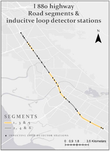
Can we use subjective knowledge by applying linguistic rules to model real traffic and indicate congestion? To test this, we are utilizing the Mobile Century (Herrera et al. 2010) data, which was collected on 8 February 2008 on Interstate 880, as part of a joint UC Berkeley–Nokia project. The California Department of Transportation funded it to support the exploration of uses of GPS enabled phones to monitor traffic. In addition to the cell phone GPS data, two additional data sources are available for the experiment site. Inductive loop detector data obtained through the Freeway Performance Measurement System (PeMS), and travel time data obtained through vehicle re–identification using high-resolution video data are included with this release. For our analyses, we use the Inductive Loop Detector Data only (Table 1). Twenty-seven stations collect flow and occupancy data for each lane every 30 seconds. We use a subset of the dataset with the time interval between 6pm and 9pm.

Table 1. Description of the data.

pems_id	Vehicle Detector Station ID of the loop detector station in the PeMS database
lat, lon	Approximate latitude and longitude of the loop detector stations
Flows	Vehicle count per lane over 30 second period
Occs	Occupancy of the sensor per lane over a 30 second period

Total length of the observed highway segment is 18 km. Figure 1 shows the area of interest (I 880 highway), with road segments and locations of inductive loop detector stations. We divide the highway stretch on six segments and calculate the average level of congestion at each segment during the time interval between 6pm and 9pm. The road segments are not of the same length, but rather follow the constitution of detector loops. The segment ends before the highway entrance, or starts after exit, depending on where the station is placed. Additionally, we observe congestion behaviour in each of four lanes individually.

Figure 1. The stretch of highway I 880 at which the mobile century experiment took place, with road segments and locations of inductive loop detectors.

The first step in building our fuzzy inference model is to specify models’ both input and output parameters. We choose to use two input parameters (traffic flow and density) and one output (level of congestion). Flow refers to the number of vehicles that passes a certain cross section per time unit (in this case 30 seconds’ period). The data, for all four lanes, is obtained from loop detector stations and for this purpose used in its original form. Density represents number of cars passing through a specific location (latitude and longitude of the Loop Detector Stations on the highway I 880, direction Northbound) at the specific time interval (here time interval equals 30 seconds). Since our dataset does not provide information about density, we calculate traffic density using data coming from traffic detectors. If we assume that all vehicles are of the same length, we get a relation between relative occupancy (b) and density (k):

(2) $\mathrm{b}={\mathrm{L}}^{\mathrm{x}}\mathrm{k}$(2)

where L is the length of the vehicles (we use length of 4 m as a standard). As for the output parameter, level of congestion we define it in the first step as well, while more attention is given to it in further steps.

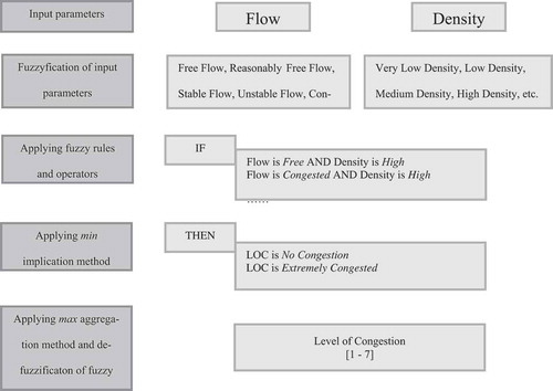
In the second step, we fuzzyfy both input and one output parameters by assigning them seven membership functions. For all input and output parameters, six full-triangle membership functions describe the middle range of the universe of discourse and one half triangle membership function represents the end of the domain of discourse, respectively. These neighbouring membership functions overlap with each other by 20–50%. The input parameter – Flow – is assigned with the following linguistic variables: Free Flow, Reasonably Free Flow, Stable Flow, Unstable Flow, Near-congestion Flow, Congested Flow and Extremely Congested Flow. The input parameter – Density – is fuzzyfied as: Very Low Density, Low Density, Medium Density, High Density, Very High Density, Extreme Density and Over Extreme Density. The output parameter – Level of Congestion – (calculated for each road segment and lane individually) is also fuzzyfied with seven linguistic variables. Table 2 shows the interpretation of each individual level of congestion.

Table 2. Fuzzy inference model output parameter (level of congestion) interpretation set-up.

LoC 1	Completely Congestion Free
LoC 2	Congestion Free
LoC 3	Stable
LoC 4	Unstable
LoC 5	Near Congestion
LoC 6	Congestion
LoC 7	Severe Congestion

In the third step, we combine our previously fuzzyified inputs using if–then fuzzy rules. Linguistic information (such as free flow and moderate density) are connected with AND operator meaning that minimum condition has to be met in order for conditional if statement to be fulfilled. Each rule combination is evaluated parallel, applying a minimum implication operator, which truncates the output fuzzy set. There are thirty-one ‘if–then’ rule combinations in total. Selected subset of rules is listed in Table 3. In order to obtain the decision based on all rules output, the outputs need to be further combined (aggregation step). We use maximum aggregation operator to combine fuzzy outputs of each individual rule and obtain single fuzzy set output. This aggregated output fuzzy set is at the same time input parameter for the de-fuzzification process. We choose centroid de-fuzzification method that gives us the average of the maximum value of the output set.

Table 3. Fuzzy if–then rules with AND operator.

IF	AND	THEN
Flow is Free Flow		Density is Very Low	LOC is LOC1
Flow is Free Flow		Density is Low	LOC is LOC2
Flow is Stable Flow		Density is Low	LOC is LOC2
Flow is Stable Flow		Density is High	LOC is LOC4
Flow is Unstable Flow		Density is High	LOC is LOC5
Flow is Congested Flow		Density is Moderate	LOC is LOC4
Flow is Heavy Congested Flow		Density is Extreme	LOC is LOC7

A schematic view of our proposed fuzzy inference model is shown in Figure 2. The figure shows the structure of the model, with input parameters, assigned linguistic variables to our crisp inputs, applied fuzzy rules and operators, chosen implication and aggregation method as well as calculated value of congestion as a defuzzified output.

Figure 2. Fuzzy inference model with two input variables (flow and density of the vehicles) and one output (level of congestion).

In the fourth and final step, we run our model with all specified parameters and export the results, separately for all four lanes. This results in particular values for flow, density and level of congestion. Table 4 shows the subset of the obtained results. It is important to note that the closer the value to zero, the less congested the segment is and vice versa – the closer to one, the more congested it gets.

Table 4. Table view of the fuzzy inference model input variables (flow and density) and output variable (level of congestion) where levels of congestion closer to 0 indicate congestion free zones and closer to 1 severe congestion zones.

Flow	Density	Level of Congestion
11	17.2	0.65
14	38.9	0.9
14	42.6	0.9
9	107.4	0.5

Based on these outputs, we are able to observe traffic behaviour at the small segment of the highway I 880, direction Northbound where the experiment took place. The maps depicted in Figure 3 show the detected levels of congestion at the segmented highway section, in each lane separately.

Figure 3. Levels of congestion detected between 6pm and 9pm on 8 February 2008, stretch of highway I 880 – northbound direction, in all four lanes.

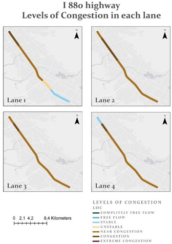
We notice that detected levels of congestion do not differ a lot among each other. There is a smooth transition from stable flow to noticeable congestion in all four lanes (south–east to north–west direction). Lane 1 has slightly lower detected CIs, compared to the rest three lanes. Additionally, lane 4 has an interesting decrease in traffic flow from segment 5 to segment 6 jumping from extreme congestion to unstable flow.

Congestion observation within segments shows similar pattern, with mostly near congestion to congested levels. Somewhat different are segment 1 at lane 1 and segment 6 at lane 4, which show rather stable flows. We observe the behaviour and occurrence of the traffic congestion on an hourly level (namely 6–7pm, 7–8pm, 8–9pm). The results revile that there is no evident difference in congestion behaviour compared to the three hour period (6–9pm). Detected levels of congestion on an hourly level show similar pattern that we already observe in Figure 3. All lanes have smooth transition between near to congestion and congestion condition.

Discussion and conclusions – effectiveness of a fuzzy inference model

After defining input variables, we need to calculate the traffic density values from the row data sample. Since our data contains the information of relative occupancy at the specific location, we are able to derive the information about densities (Equation 1.2). We assume, additionally, that all vehicles have the same length. However, traffic stream is rarely homogeneous in reality and vehicles are, usually, not of the same length. Better solution for finding traffic density using traffic detectors, would be to measure the flow rate and mean speed, and then calculate density using the fundamental relation (Equation 1.1). The second input variable for the fuzzy inference model is flow. Loop detectors across the study area provide vehicle counts per lane over 30 second period. Given that the total flow, expected on the section of interest, is approximately 6000 vehicles per hour (from PeMS) we assume that capacity of each lane is equal and amounts to 1500 vehicles per hour (~13 vehicles per 30s period). This normalized approach might cause results misinterpretation, which we cannot detect.

We use two input variables to describe traffic congestion – flow and density. These have proven to be sufficient for the fuzzy inference model. Most likely more factors determine this phenomenon and as such needs to be included into the model. Very often, different weights are assigned to different parameters, depending on their influence on observed event. In our example, we assume that both flow and density are weighted the same (even though flow information is provided and density information is calculated accounting for homogeneous traffic conditions) which might vary depending on the road conditions within the case study area. In addition, we specify arbitrary number of if–then rules based on existing literature review recommendations and our personal experience as traffic participants. This step in building a fuzzy inference model needs to be further investigated and improved by extending the knowledge about the data and the study area. Additionally, used data refer only to a very short time interval between 6pm and 9pm when levels of traffic congestions are generally smoother than during the peak hours. The strength of the fuzzy model could be better observed and evaluated if more data is fed into the system.

In contrast to traditional methods of detecting traffic congestion, we use rather approximate approach. Our fuzzy inference model does not consider nor rely on the exact numbers to derive conclusions (e.g. the exact count of vehicles within the road segment implies how congested specific segment is). On the contrary, this approach is based on natural language (linguistic information) rules, which are consistent with the general feelings of traffic participants. Since more than single rule is applied in the inference system (multiple rules describe given situation), derived conclusion is a composite image of traffic conditions. Additionally, the proposed method is simple to apply and follows common sense logic. We believe that this viewpoint presents a promising approach in modelling traffic and transportation processes because of its flexibility in dealing with subjectivity, ambiguity, imprecision and uncertainty. Our goal here is to introduce our own approach, based on own knowledge and available study data, to be further improved and utilized for obtaining more accurate traffic events prognosis. In future steps, we plan to extend the model with other relevant measures (such as mean speed or velocity), as well as to improve model performance through more sophisticated fuzzy rules assignment.

Data availability statement

The data that support the findings of this study are openly available at http://traffic.berkeley.edu/project/downloads/mobilecenturydata. By downloading the data, the user acknowledges that the data would be:

1. Used only for research and analysis purposes.

2. Will not be distributed further.

3. Any publication using the data should refer to the following article: Herrera et al. (2010) Evaluation of traffic data obtained via GPS-enabled mobile phones: The Mobile Century field experiment. Transportation Research Part C: Emerging Technologies. Pergamon, 18(4): 568–583. doi: 10.1016/J.TRC.2009.10.006.

Disclosure statement

No potential conflict of interest was reported by the authors.

References

- Aftabuzzaman, M. 2007. “Measuring Traffic Congestion - A Critical Review.” 30th Australasian Transport Research Forum. Accessed 30 November 2018. https://scholar.google.com/scholar?as_q=Measuring+traffic+congestion%3A+A+critical+review&as_occt=title&hl=en&as_sdt=0%2C31
- D’Este, G., R. Zito, and M. Taylor. 1999. “Using GPS to Measure Traffic System Performance.” Computer - Aided Civil and Infrastructure Engineering. 14 (4): 255–265. doi:10.1111/0885-9507.00146.
- Downs, A. 2004. “Why Traffic Congestion Is Here to Stay … and Will Get Worse.” ACCESS Magazine 1 (25): 19–25. Accessed 30 November 2018. https://escholarship.org/uc/item/3sh9003x
- Fullér, R., and H. Zimmermann. 1993. “Fuzzy Reasoning for Solving Fuzzy Mathematical Programming Problems.” Fuzzy Sets and Systems 60 (3): 121–133. Accessed 30 November 2018. https://pdfs.semanticscholar.org/0ca9/bb36a2b7917f2652ac1062ad25c37dacc97b.pdf
- Herrera, J.,Work, D. B., Herring, R., Ban, X. J., Jacobson, Q., and Bayen, A. M. 2010. “Evaluation of Traffic Data Obtained via GPS-enabled Mobile Phones: The Mobile Century Field Experiment. Transportation Research Part C: Emerging Technologies.” Pergamon 18 (4): 568–583. doi:10.1016/J.TRC.2009.10.006.
- Immers, L., and S. Logghe. 2008. “Multi-class Kinematic Wave Theory of Traffic Flow. Transportation Research Part B: Methodological.” Pergamon 42 (6): 523–541. doi:10.1016/J.TRB.2007.11.001.
- Kockelman, K. 2004. “Traffic Congestion.” In Handbook of Transportation Engineering Chapter 12: Traffic Congestion, edited by K. Myer. pp. 1-20. New York: McGraw-Hill.
- Krause, B., C. von Altrock, and C. Pozybill. 1996. “Intelligent Highway by Fuzzy Logic: Congestion Detection and Traffic Control on Multi-lane Roads with Variable Road Signs.” In Proceedings of IEEE 5th International Fuzzy Systems, pp. 1832–1837. New Orleans, USA. IEEE. doi: 10.1109/FUZZY.1996.552649.
- Lee, C. C. 1990. “Fuzzy Logic in Control Systems: Fuzzy Logic Controller-Part I and Part H.” IEEE Transactions on Systems Man and Cybernetics 20 (2): 404–435.
- Lomax, T. 1997. “Quantifying Congestion.” NCHRP Report. Washington, DC: Transportation Research Board. Accessed 30 November 2018. http://onlinepubs.trb.org/onlinepubs/nchrp/nchrp_rpt_398.pdf
- Mamdani, E. H., and S. Assilian. 1975. “An Experiment in Linguistic Synthesis with a Fuzzy Logic Controller.” International Journal of Man-Machine Studies 7 (1): 1–13. doi:10.1016/S0020-7373(75)80002-2.
- May, A. 1990. Traffic Flow Fundamentals. New Jersey: Prentice Hall, Englewood Cliffs.
- Mendel, J. 1995. “Fuzzy Logic Systems for Engineering.” Proceedings of the IEEE 83: 345–377. doi:10.1109/5.364485.
- Miller, M. A., and K. Li. 1994. “An Investigation of the Costs of Roadway Traffic Congestion: Preparatory Step for IVHS Benefit’s Evaluation.” UC Berkeley - California Partners for Advanced Transportation Technology. Accessed 30 November 2018. https://escholarship.org/uc/item/1zk368mg
- Nakatsuyama, M., H. Nagahashi, and N. Nishizuka. 1984. “Fuzzy Logic Phase Controller for Traffic Junctions in the One-way Arterial Road.” Proceedings of 9th International Federation of Automatic Control World Congress 17 (2): 2865–2870. doi:10.1016/S1474-6670(17)61417-4.
- Pappis, C. P., and E. H. Mamdani. 1977. “A Fuzzy Logic Controller for A Trafc Junction.” IEEE Transactions on Systems, Man, and Cybernetics 7 (10): 707–717. doi:10.1109/TSMC.1977.4309605.
- Rosenbloom, S. 1978. “Peak-period Traffic Congestion: A State-Of-the-art Analysis and Evaluation of Effective Solutions.” Transportation. Kluwer Academic Publishers 7 (2): 167–191. doi:10.1007/BF00184638.
- Sasaki, T., and T. Akiyama. 1986. “Development of Fuzzy Traffic Control System on Urban Expressway.” In Control in Transportation Systems 1st Edition - Proceedings of the 5th IFAC/IFIP/IFORS Conference, Vienna, Austria, 8-11 July 1986, edited by R. Genser, T. Hasegawa, M.M. Etschmaier and H. Strobel, 215–220. doi:10.1016/B978-0-08-033438-7.50040-9.
- Sasaki, T., and T. Akiyama. 1987. “Fuzzy On-ramp Control Model on Urban Expressway and Its Extension.” In Transportation and Traffic Theory, edited by N. Gartner and N. Wilson, 377–395. New York: Elsevier Science.
- Sasaki, T., and T. Akiyama. 1988. “Traffic Control Process of Expressway by Fuzzy Logic.” Fuzzy Sets and Systems North-Holland. 26 (2): 165–178. doi:10.1016/0165-0114(88)90206-0.
- Schrank, D., and T. Lomax. 1997. “Urban Roadway Congestion: 1982–1994.” Research Report 1: 1131–1139. Accessed 30 November 2018. https://static.tti.tamu.edu/tti.tamu.edu/documents/1131-9-V1.pdf
- Sugeno, M. 1985. “An Introductory Survey of Fuzzy Control.” Information Sciences 36: 59–83. doi:10.1016/0020-0255(85)90026-X.
- Sugeno, M., and M. Nishida. 1985. “Fuzzy Control of Model Car. In: Fuzzy Sets and Systems.” North-Holland 16 (2): 103–113. doi:10.1016/S0165-0114(85)80011-7.
- Taylor, M. A. P. 1992. “Exploring the Nature of Urban Traffic Congestion: Concepts, Parameters, Theories and Models.” Proceedings of 16th Australian Road Research Board Conference 16 (5): 83–105. Perth: ARRB.
- Victoria Transport Policy Institute - VTPI. 2005. “Congestion Reduction Strategies: Identifying and Evaluating Strategies to Reduce Congestion.” In Online TDM Encyclopaedia, Victoria. British Columbia, Canada: Victoria Transport Policy Institute. Accessed 30 November 2018. https://www.vtpi.org/tdm/tdm96.htm
- Wardrop, J. G. 1952. “Some Theoretical Aspects of Road Traffic Research.” Proceedings of the Institution of Civil Engineers 1 (3): 325–362. doi:10.1680/ipeds.1952.11259.
- Weisbrod, G., D. Vary, and G. Treyz. 2001. “Economic Implications of Congestion.” In National Cooperative Highway Research Program - NCHRP Report 463, 1-55. National Academy Press, Washington DC. Accessed 30 November 2018. http://onlinepubs.trb.org/onlinepubs/nchrp/nchrp_rpt_463-a.pdf
- Zadeh, L. A. 1973. “Outline of a New Approach to the Analysis of Complex Systems and Decision Processes.” IEEE Transactions on Systems, Man, and Cybernetics - SMC 3 (1): 28–44. doi:10.1109/TSMC.1973.5408575.