An evaluation of the efficiency of similarity functions in density-based clustering of spatial trajectories

ABSTRACT

Spatiotemporal movement pattern discovery has stimulated considerable interest due to its numerous applications, including data analysis, machine learning, data segmentation, data reduction, abnormal behaviour detection, noise filtering, and pattern recognition. Trajectory clustering is among the most widely used approaches of extracting interesting patterns in large trajectory datasets. In this paper, regarding the optimal performance of density-based clustering, we present a comparison between eight similarity measures in density-based clustering of moving objects’ trajectories. In particular, Distance Functions such as Euclidean, L1, Hausdorff, Fréchet, Dynamic Time Warping (DTW), Longest Common SubSequence (LCSS), Edit Distance on Real signals (EDR), and Edit distance with Real Penalty (ERP) are applied in DBSCAN on three different datasets with varying characteristics. Also, experimental results are evaluated using both internal and external indices. Furthermore, we propose two modified validation measures for density-based trajectory clustering, which can deal with arbitrarily shaped clusters with different densities and sizes. These proposed measures were aimed at evaluating trajectory clusters effectively in both spatial and spatio-temporal aspects. The evaluation results show that choosing an appropriate Distance Function is dependent on data and its movement parameters. However, in total, Euclidean distance proves to show superiority over the other Distance Functions regarding the Purity index and EDR distance can provide better performance in terms of spatial and spatio-temporal quality of clusters. Finally, in terms of computation time and scalability, Euclidean, L1, and LCSS are the most efficient Distance Functions.

KEYWORDS:

• Spatial trajectories
• clustering
• distance functions
• spatio-temporal similarity
• DBSCAN

1. Introduction

Remarkable developments in information and communication technologies such as wireless networks and mobile computing devices along with the significant increase in accuracy of positioning services have led to the collection of massive volumes of moving objects’ trace data. Performing data analysis over traces of moving objects, e.g. citizens, vehicles, and animals leads to useful information about movement patterns. Pattern extraction play an essential role in many applications including traffic control, urban planning, smart transportation, and biological studies (Basiri, Amirian, and Mooney 2016; Yuan et al. 2017; Zheng et al. 2009; Mahdavinejad et al. 2018) which has captured lots of attention over the last two decades.

The term spatial trajectory refers to a special kind of time series in which the location of a moving object has been captured at specific instances of time (Georgiou et al. 2018). Generally, spatial trajectories are represented by a sequence of timestamped locations as follows (Aghabozorgi, Shirkhorshidi, and Wah 2015):

(1) ${\mathrm{P}}_{\mathrm{k}}=\left(\mathrm{i}{\mathrm{d}}_{\mathrm{k}},\mathrm{l}\mathrm{o}{\mathrm{c}}_{\mathrm{k}},{\mathrm{t}}_{\mathrm{k}},{\mathrm{A}}_{\mathrm{k}}\right),\mathrm{i}\mathrm{n}\mathrm{t}\mathrm{h}\mathrm{e}{\mathrm{k}}^{\mathrm{t}\mathrm{h}}\mathrm{t}\mathrm{i}\mathrm{m}\mathrm{e}$(1)

where id_k is the location identifier, loc_k is the position at the time t_k, and A_k is other descriptive data related to the point.

In order to extract useful patterns out of trajectory data with huge volume, different methods such as clustering and classification are usually applied. Clustering is an unsupervised learning method, associating data in groups (clusters) based on their distance. (Han, Pei, and Kamber 2011; Xu and Wunsch 2005). The aim of trajectory clustering is categorizing a trajectory dataset in groups of clusters based on their movement characteristics. Trajectories existing in each cluster have similar movement characteristics or behaviour to one another within the same cluster and dissimilar to the trajectories in other clusters (Berkhin 2006; Besse et al. 2015; Yuan et al. 2017).

Generally, two main approaches can be employed for clustering complex data like trajectories. First, defining trajectory-specific clustering algorithms and second, using generic clustering algorithms which utilizes trajectory-specific Distance Functions (DFs). The latter encapsulated the specifics of the trajectory data are in DFs (Andrienko and Andrienko 2010). Some generic clustering algorithms like K-means are only able to extract clusters with a convex shape, and they are also unstable against outliers. However, it is clear that trajectory clusters are of arbitrary shape (concave, drawn-out, linear, elongated), and their datasets are much capable of having outliers. One of the most suitable clustering methods for trajectories is density-based clustering (Kriegel et al. 2011) which can extract clusters with arbitrary shape and is also tolerant against outliers(Ester et al. 1996). Density-Based Spatial Clustering of Applications with Noise (DBSCAN) is one of the most popular methods among this family, which is widely employed in trajectory clustering (Zhao and Shi 2019; Cheng et al. 2018; Chen et al. 2011b; Lee, Han, and Whang 2007).

Measuring the similarity is the central core of the clustering problem; therefore, similarity (inverse of distance) should be determined before grouping. Distance definition in spatial trajectories is much more complicated than point data. Trajectories are sequences of points in several dimensions that are not of the same length. Thus, in order to compare two trajectories, a comprehensive approach is needed to fully determine their distance. Depending on the analysis purpose and also the data type, different DFs are presented. The concept of similarity is domain specific, so different DFs is defined in order to address different aspects of similarity such as spatial, spatio-temporal, and temporal.

Spatial similarity is based on spatial parameters like movement path and its shape whereas spatio-temporal similarity is based on movement characteristics like speed, and temporal similarity is based on time intervals and movement duration (Ranacher and Tzavella 2014). For instance, in order to extract the movement patterns in trajectories like detecting the transportation mode, besides the trajectories geometry, their movement parameters should also be considered. Accordingly, every distance function is not suitable for all applications, and correct recognition of data and application is crucial.

Among all defined Distance Functions so far, Euclidean, Fréchet, Hausdorff, DTW, LCSS, EDR, and ERP distances are the basic functions in similarity measurements from which so many other functions are generated (Aghabozorgi, Shirkhorshidi, and Wah 2015; Wang et al. 2013; Ali Abbaspour, Shaeri, and Chehreghan 2017).

Validation is widely considered as the most challenging and vital factor in clustering. The present paper aims to evaluate the effect of different DFs in clustering methods, which are based on density in spatial trajectories. Considering the fact that in previous research density-based methods performed better in trajectory clustering than other methods (Birant and Kut 2007; Zhang et al. 2014), finding a DF with the best efficiency among this type of clustering functions is an essential issue that, no one to the best of our knowledge has studied it. In order to fulfil this aim, the effectiveness of some frequently used DFs is evaluated in DBSCAN clustering algorithm. For the correct selection of similarity functions to be used in DBSCAN, the results of each algorithm are compared to Purity index, Spatial CS measure, and Spatio-temporal to find out to which of the distance functions the DBSCAN algorithm shows a more efficient reaction. The current research attempts to reach the intended results by contributing to the following aspects compared to the previous studies:

• Using datasets with different movement parameters and varying complexities for studying the effect of data variety

• Studying the effect of different values of noise and outliers

• Using both internal and external indicators to evaluate the quality of clustering

• Suggesting two modified validation measures for density-based trajectory clustering to meet both spatial and spatio-temporal quality of clusters

• Comparing the operational time of different similarity functions and assessing the effect of the increase in the data volume on it.

This paper continues as follows: after the introduction, Section 2 gives a brief overview of the literature review. Theoretical foundations and suggested method are detailed in Section 3. Section 4 begins by describing the data under study and continues with examining the applied framework on this data. Finally, the paper is ended with some conclusions and suggestions in Section 5.

2. Literature review

Up to now, numerous Distance Functions have been proposed that each one makes use of a different definition of similarity in trajectories. The most basic Distance Function is Euclidean distance. Clarke (1976), Richalet et al. (1978), and Takens (1980) have made use of this distance for studying the similarity in trajectories. Myers, Rabiner, and Rosenberg (1980) pioneered in employing DTW, another important DF, to compute the time series distance. Besides, Kruskal (1983) and Picton et al. (1988) exploited this algorithm for measuring the spatial trajectory distance. Concerning the nature of spatio-temporal data, which contains noise and outliers, developing DFs which were more robust against these errors was reasonable. Therefore, some DFs were proposed based on the LCSS by Kearney and Hansen (1990) and Vlachos, Kollios, and Gunopulos (2002a).

In addition to the research mentioned above in suggesting new DFs, several studies were also conducted on comparing and evaluating the similarity functions. Wang et al. (2013) widely investigated the weaknesses and strengths of six DFs including Euclidean, DTW, PDTW, EDR, ERP, and LCSS distances for the measurement of trajectory similarity by applying different transformations. They have identified DTW as the superior DF, and LCSS as the only resistant DF against noise and inconstant sampling rate. However, the effect of distance functions in trajectory clustering is not investigated.

Despite the considerable amount of literature on defining Distance Functions and evaluating them, not much is known about the performance of DFs in spatial trajectory clustering. Atev, Miller, and Papanikolopoulos (2010) compared the performance of their suggested edited Hausdorff function to two basic DFs, DTW and LCSS, in trajectory clustering by hierarchical and spectral methods and concluded that their proposed function has superiority over those two basic DFs. However, the effect of other important Distance Functions like Euclidean distance, L1 Norm, Hausdorff, Fréchet, EDR, and ERP in clustering has not been addressed. Besse et al. (2016) conducted an assessment of the performance of their suggested DF (SSPD) and some known DFs (DTW, LCSS, ERP, Hausdorff, Fréchet, Discrete Fréchet, and OWD) in two clustering methods of hierarchical and affinity propagation. They claimed that the best results had been achieved from OWD, and on the other hand, LCSS had shown a weak performance.

Much work on the evaluation of geometrical similarity function has been carried out, yet there are still some critical issues about movement similarity parameters like velocity, acceleration, direction, and complexity. For many application domains, however, the geometrical similarity is insufficient for an in-depth understanding of the motion of moving objects. For instance, in order to group the pedestrians in a sidewalk and to distinguish the ones who walk from the ones who run, the use of geometrical similarity will not lead to consistent results, and it is crucial to consider the speed similarity and speed changes during time. Each type of measures has advantages and disadvantages, and that which one is better suited in the domain of density-based trajectory clustering is the central question that is addressed in this paper.

Our paper aims to present a comprehensive comparison of the performance of the similarity functions in trajectory clustering and on data with different complexities which contain noise and outliers based on three criteria: clustering quality, our proposed velocity coefficient, and the computational time, which has not been addressed in previous studies.

3. Methodology

In this section, we propose a framework that summarizes the whole procedure of evaluating the performance of Distance Functions in density-based clustering, as shown in Figure 1.

Figure 1. A general flowchart for assessment of distance functions in density-based clustering.

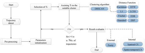
In the initial stage of the process, experimental data with different movement characteristics are selected in order to do the secondary analysis. In the pre-processing stage, noise and outliers with different values are applied to the original data in order to evaluate the effect of the error on the performance of Distance Functions in density-based trajectory clustering. The process of trajectory clustering with DBSCAN algorithm using Euclidean, L1, Hausdorff, Fréchet, DTW, LCSS, EDR, and ERP distances is presented in the following part. In the next step, the efficiency of each DF in density-based clustering is evaluated using internal and external indicators and the computational time.

3.1. Distance functions

3.1.1. Euclidean distance

The Euclidean distance is a traditional distance which is employed in various areas of data mining like determining the trajectory similarity. Among all advantages of this DF, the simplicity of implementation, low computation time, and not requiring the initial parameter can be mentioned. However, its result is considerably sensitive to the presence of noise and outliers. Moreover, it requires trajectories to be the same length and be sampled at fixed time intervals. (Pfeifer and Deutrch 1980; Priestley 1980). To overcome these stated drawbacks, other DFs were defined that will be discussed later. Given two trajectories L_i and L_j of length n in p dimension, the Euclidean distance between them, DE (L_i, L_j), is defined as Formula 2.

(2) ${\mathrm{D}}_{\mathrm{E}}\left({\mathrm{L}}_{\mathrm{i}},{\mathrm{L}}_{\mathrm{j}}\right)=\frac{1}{\mathrm{n}}\sum _{\mathrm{k}=1}^{\mathrm{n}}\sqrt{\sum _{\mathrm{m}=1}^{\mathrm{p}}{\left({\mathrm{a}}_{\mathrm{k}}^{\mathrm{m}}-{\mathrm{b}}_{\mathrm{k}}^{\mathrm{m}}\right)}^2}$(2)

where, ${\mathrm{a}}_{\mathrm{k}}^{\mathrm{m}}$ is the m^th dimension of the k^th point of L_i.

3.1.2. Norm L1

Norm L1 is similar to the Euclidean distance except that it is more robust to noise. Lp-norms are easy to compute. However, they cannot handle local time-shifting, which is essential in trajectory similarity measurement. The calculation of this distance is detailed in Equation (3). Parameters used in this equation are defined in the same way as Equation (2) (Jajuga 1987).

(3) ${\mathrm{D}}_{\mathrm{L}}\left({\mathrm{L}}_{\mathrm{i}},{\mathrm{L}}_{\mathrm{j}}\right)=\frac{1}{\mathrm{n}}\sum _{\mathrm{k}=1}^{\mathrm{n}}\sqrt{\sum _{\mathrm{m}=1}^{\mathrm{p}}|{\mathrm{a}}_{\mathrm{k}}^{\mathrm{m}}-{\mathrm{b}}_{\mathrm{k}}^{\mathrm{m}}|}$(3)

3.1.3. Hausdorff distance

Hausdorff distance is another function for calculating the closeness of two trajectories or a subset of them. Two trajectories are defined as close if each one of the first trajectory points is proximate to at least one point of the second trajectory (Wei et al. 2013). To calculate the Hausdorff distance, Equation (4) is used (Chen et al. 2011a).

(4) ${\mathrm{D}}_{\mathrm{H}}\left({\mathrm{L}}_{\mathrm{i}},{\mathrm{L}}_{\mathrm{j}}\right)=\mathrm{m}\mathrm{a}\mathrm{x}(\mathrm{h}\left({\mathrm{L}}_{\mathrm{i}},{\mathrm{L}}_{\mathrm{j}}\right),\mathrm{h}\left({\mathrm{L}}_{\mathrm{j}},{\mathrm{L}}_{\mathrm{i}}\right))$(4)

where h(L_i, L_j) is calculated from Equation (5).

(5) $\mathrm{h}\left({\mathrm{L}}_{\mathrm{i}},{\mathrm{L}}_{\mathrm{j}}\right)=\mathrm{m}\mathrm{a}{\mathrm{x}}_{\mathrm{a}\in {\mathrm{L}}_{\mathrm{i}}}\left(\mathrm{m}\mathrm{i}{\mathrm{n}}_{\mathrm{b}\in {\mathrm{L}}_{\mathrm{j}}}\left(\mathrm{e}\mathrm{u}\mathrm{c}\left(\mathrm{a},\mathrm{b}\right)\right)\right)$(5)

In Equation (5), euc (a, b) is the Euclidean distance between the sampled points a and b which belong to trajectories L_i and L_j respectively.

3.1.4. Fréchet distance

This function emphasizes on the location as well as the order of points in the sequence for measuring the similarities. Fréchet distance searches all the points in both trajectories to find the longest Euclidean distance between two trajectories (Alt and Godau 1995). Fréchet distance between two trajectories L_i and L_j are given by Equation (6) (Khoshaein 2013).

(6) ${\mathrm{D}}_{\mathrm{F}}\left({\mathrm{L}}_{\mathrm{i}},{\mathrm{L}}_{\mathrm{j}}\right)=\mathrm{m}\mathrm{i}\mathrm{n}\left\{\left|\left|\mathrm{c}\right|\right|,\mathrm{c}\mathrm{i}\mathrm{s}\mathrm{c}\mathrm{o}\mathrm{u}\mathrm{p}\mathrm{l}\mathrm{i}\mathrm{n}\mathrm{g}\mathrm{b}\mathrm{e}\mathrm{t}\mathrm{w}\mathrm{e}\mathrm{e}\mathrm{n}{\mathrm{L}}_{\mathrm{i}}\mathrm{a}\mathrm{n}\mathrm{d}{\mathrm{L}}_{\mathrm{j}}\right\}$(6)

where ||c|| is calculated by Equation (7).

(7) $\left|\left|\mathrm{c}\right|\right|={\mathrm{m}\mathrm{a}\mathrm{x}}_{\mathrm{k}=1}^{\mathrm{K}}\mathrm{e}\mathrm{u}\mathrm{c}\left({\mathrm{a}}_{\mathrm{i}}^{\mathrm{k}},{\mathrm{b}}_{\mathrm{j}}^{\mathrm{k}}\right)$(7)

where L_i and L_j are two trajectories of m and n lengths and K = min(m,n). ${\mathrm{a}}_{\mathrm{i}}^{\mathrm{k}}$ and ${\mathrm{b}}_{\mathrm{j}}^{\mathrm{k}}$ are the k^th points of L_i and L_j trajectories, respectively.

3.1.5. DTW

DTW is a popular DF for finding the optimal queueing between two time series, and it is employed for evaluating the similarity in trajectories having even different lengths. Its primary purpose is to find the path w between two trajectories with the lowest cost. Compared to Euclidean distance and norm L1, among the advantages of this method, more stability because of independence from local time shifting as well as finding the optimal path even with temporal stretch and the different sampling rate can be mentioned (Kruskal 1983; Myers, Rabiner, and Rosenberg 1980). DTW distance between two trajectories L_i and L_j of lengths m and n, respectively, is defined by Equation (8) (Berndt and Clifford 1994).

(8) ${\mathrm{D}}_{\mathrm{D}\mathrm{T}\mathrm{W}}\left({\mathrm{L}}_{\mathrm{i}},{\mathrm{L}}_{\mathrm{j}}\right)=\left\{\begin{array}{c}0,\mathrm{m}=\mathrm{n}=0\\ \mathrm{\infty },\mathrm{m}=0||\mathrm{n}=0\\ \mathrm{e}\mathrm{u}\mathrm{c}\left({\mathrm{a}}_{\mathrm{i}}^{\mathrm{k}}{,\mathrm{b}}_{\mathrm{j}}^{\mathrm{k}}\right)+\mathrm{m}\mathrm{i}\mathrm{n}\left\{\begin{array}{c}{\mathrm{D}}_{\mathrm{D}\mathrm{T}\mathrm{W}}\left(\mathrm{R}\left({\mathrm{L}}_{\mathrm{i}}\right),\mathrm{R}\left({\mathrm{L}}_{\mathrm{j}}\right)\right),\\ {\mathrm{D}}_{\mathrm{D}\mathrm{T}\mathrm{W}}\left(\mathrm{R}\left({\mathrm{L}}_{\mathrm{i}}\right),{\mathrm{L}}_{\mathrm{j}}\right),\\ {\mathrm{D}}_{\mathrm{D}\mathrm{T}\mathrm{W}}\left({\mathrm{L}}_{\mathrm{i}},\mathrm{R}\left({\mathrm{L}}_{\mathrm{i}}\right)\right)\end{array}\right\},\mathrm{o}\mathrm{t}\mathrm{h}\mathrm{e}\mathrm{r}\end{array}\right.$(8)

where, R(L_i) and R(L_j) are the remained trajectory from L_i and L_j, respectively, after removing their initial points.

3.1.6. LCSS

The LCSS is a variation of the Edit Distance which calculates the size of the longest similar substring in two trajectories. This function contains two threshold values of σ and ɛ, which are used in x and y directions respectively. When the difference between x and y of two points in two trajectories is less than the threshold extent, these pairs of points are assumed similar, and LCSS is increased by one unit. Unlike Euclidean and DTW, LCSS attempts to match two trajectories by enabling them to stretch, without rearranging the sequence of the elements, however allowing some elements to be unmatched, which makes it very robust to noise (Vlachos, Kollios, and Gunopulos 2002b). LCSS distance between two trajectories L_i and L_j are given by Equation (9) (Rick 2000).

(9) ${\mathrm{D}}_{\mathrm{L}\mathrm{C}\mathrm{S}\mathrm{S}}\left({\mathrm{L}}_{\mathrm{i}},{\mathrm{L}}_{\mathrm{j}}\right)=\left\{\begin{array}{c}0,\mathrm{m}=\mathrm{n}=0\\ 1+{\mathrm{D}}_{\mathrm{L}\mathrm{C}\mathrm{S}\mathrm{S}}\left(\mathrm{R}\left({\mathrm{L}}_{\mathrm{i}}\right),\mathrm{R}\left({\mathrm{L}}_{\mathrm{j}}\right)\right),\left|{\mathrm{a}}_{\mathrm{i}}^{\mathrm{x}}{-\mathrm{b}}_{\mathrm{j}}^{\mathrm{x}}\right|\pounds \sigma \mathrm{a}\mathrm{n}\mathrm{d}\left|{\mathrm{a}}_{\mathrm{i}}^{\mathrm{y}}{-\mathrm{b}}_{\mathrm{j}}^{\mathrm{y}}\right|\le \epsilon \\ \mathrm{m}\mathrm{a}\mathrm{x}\left\{\begin{array}{c}{\mathrm{D}}_{\mathrm{L}\mathrm{C}\mathrm{S}\mathrm{S}}\left(\mathrm{R}\left({\mathrm{L}}_{\mathrm{i}}\right),{\mathrm{L}}_{\mathrm{j}}\right),\\ {\mathrm{D}}_{\mathrm{L}\mathrm{C}\mathrm{S}\mathrm{S}}\left({\mathrm{L}}_{\mathrm{i}},\mathrm{R}\left({\mathrm{L}}_{\mathrm{i}}\right)\right)\end{array}\right\},\mathrm{O}\mathrm{t}\mathrm{h}\mathrm{e}\mathrm{r}\end{array}\right.$(9)

where ε and σ are the required initial parameters of the equation which should be determined by the user. ${\mathrm{a}}_{\mathrm{i}}^{\mathrm{x}}$ and ${\mathrm{a}}_{\mathrm{i}}^{\mathrm{y}}$ are x and y coordinate of the first point of L_i respectively where ${\mathrm{b}}_{\mathrm{j}}^{\mathrm{x}}$ and ${\mathrm{b}}_{\mathrm{j}}^{\mathrm{y}}$ are x and y coordinates of the first point of L_j respectively.

3.1.7. EDR

EDR is a similarity measure based on Edit Distance on strings, which seeks the minimum number of edit operations (e.g. replace, insert, or delete) required to change one trajectory to another. EDR is able to deal with three common problems in previous DFs, including noise, shifts, and data scaling. Given two trajectories L_i and L_j of lengths n and m, respectively, EDR distance between L_i and L_j is defined as follows (Chen, Tamer Özsu, and Oria 2005):

(10) ${\mathrm{D}}_{\mathrm{E}\mathrm{D}\mathrm{R}}\left({\mathrm{L}}_{\mathrm{i}},{\mathrm{L}}_{\mathrm{j}}\right)=\left\{\begin{array}{c}\mathrm{n},\mathrm{m}=0\\ \mathrm{m},\mathrm{n}=0\\ \mathrm{m}\mathrm{i}\mathrm{n}\left\{\begin{array}{c}{\mathrm{D}}_{\mathrm{E}\mathrm{D}\mathrm{R}}\left(\mathrm{R}\left({\mathrm{L}}_{\mathrm{i}}\right),\mathrm{R}\left({\mathrm{L}}_{\mathrm{j}}\right)\right)+\mathrm{d}\mathrm{i}\mathrm{s}\mathrm{t}\left({\mathrm{L}}_{\mathrm{i}}\left(1\right),{\mathrm{L}}_{\mathrm{j}}\left(1\right)\right),\\ {\mathrm{D}}_{\mathrm{E}\mathrm{D}\mathrm{R}}\left({\mathrm{L}}_{\mathrm{i}},\mathrm{R}\left({\mathrm{L}}_{\mathrm{j}}\right)\right)+\mathrm{d}\mathrm{i}\mathrm{s}\mathrm{t}\left(\mathrm{g}\mathrm{a}\mathrm{p},{\mathrm{L}}_{\mathrm{j}}\left(1\right)\right),\\ {\mathrm{D}}_{\mathrm{E}\mathrm{D}\mathrm{R}}\left(\mathrm{R}\left({\mathrm{L}}_{\mathrm{i}}\right),{\mathrm{L}}_{\mathrm{j}}\right)+\mathrm{d}\mathrm{i}\mathrm{s}\mathrm{t}\left({\mathrm{L}}_{\mathrm{i}}\left(1\right),\mathrm{g}\mathrm{a}\mathrm{p}\right)\end{array}\right\},\mathrm{o}\mathrm{t}\mathrm{h}\mathrm{e}\mathrm{r}\end{array}\right.$(10)

where the $\mathrm{d}\mathrm{i}\mathrm{s}\mathrm{t}\left(,\right)$ function is computed using Equation (11).

(11) $\mathrm{d}\mathrm{i}\mathrm{s}\mathrm{t}\left({\mathrm{a}}_{\mathrm{i}},{\mathrm{b}}_{\mathrm{j}}\right)=\left\{\begin{array}{c}0,\mathrm{e}\mathrm{u}\mathrm{c}\left({\mathrm{a}}_{\mathrm{i}},{\mathrm{b}}_{\mathrm{j}}\right)<\epsilon \mathrm{a}\mathrm{n}\mathrm{d}{\mathrm{a}}_{\mathrm{i}}\mathrm{a}\mathrm{n}\mathrm{d}{\mathrm{b}}_{\mathrm{j}}\mathrm{a}\mathrm{r}\mathrm{e}\mathrm{c}\mathrm{o}\mathrm{n}\mathrm{c}\mathrm{u}\mathrm{r}\mathrm{r}\mathrm{e}\mathrm{n}\mathrm{t}\\ 1,\mathrm{o}\mathrm{t}\mathrm{h}\mathrm{e}\mathrm{r}\end{array}\right.$(11)

3.1.8. ERP

ERP is a commonly used metric DF in similarity evaluation, which borrows ideas from both norm L1 and Edit Distance. Functions which are based on Lp-norms are metric; however they do not support local time shifting. On the other hand, functions based on edit distance are non-metric, but they are able to cope with local time shifting (Chen et al., 2005, 107). Given two trajectories L_i and L_j, ERP distance between L_i and L_j is:

(12) $\begin{array}{rl}& {\mathrm{D}}_{\mathrm{E}\mathrm{R}\mathrm{P}}({\mathrm{L}}_{\mathrm{i}},{\mathrm{L}}_{\mathrm{j}})=\left\{\begin{array}{c}\sum _1^{\mathrm{n}}\mathrm{e}\mathrm{u}\mathrm{c}\left({\mathrm{L}}_{\mathrm{i}}\left(\mathrm{i}\right),\mathrm{g}\mathrm{a}\mathrm{p}\right),\mathrm{m}=0\\ \sum _1^{\mathrm{m}}\mathrm{e}\mathrm{u}\mathrm{c}\left(\mathrm{g}\mathrm{a}\mathrm{p},{\mathrm{L}}_{\mathrm{j}}\left(\mathrm{j}\right)\right),\mathrm{n}=0\\ min\left\{\begin{array}{c}{\mathrm{D}}_{\mathrm{E}\mathrm{D}\mathrm{R}}\left(\mathrm{R}\left({\mathrm{L}}_{\mathrm{i}}\right),\mathrm{R}\left({\mathrm{L}}_{\mathrm{j}}\right)\right)+\mathrm{d}\mathrm{i}\mathrm{s}\mathrm{t}\left({\mathrm{L}}_{\mathrm{i}}\left(1\right),{\mathrm{L}}_{\mathrm{j}}\left(1\right)\right),\\ {\mathrm{D}}_{\mathrm{E}\mathrm{D}\mathrm{R}}\left({\mathrm{L}}_{\mathrm{i}},\mathrm{R}\left({\mathrm{L}}_{\mathrm{j}}\right)\right)+\mathrm{d}\mathrm{i}\mathrm{s}\mathrm{t}\left(\mathrm{g}\mathrm{a}\mathrm{p},{\mathrm{L}}_{\mathrm{j}}\left(1\right)\right),\\ {\mathrm{D}}_{\mathrm{E}\mathrm{D}\mathrm{R}}\left(\mathrm{R}\left({\mathrm{L}}_{\mathrm{i}}\right),{\mathrm{L}}_{\mathrm{j}}\right)+\mathrm{d}\mathrm{i}\mathrm{s}\mathrm{t}\left({\mathrm{L}}_{\mathrm{i}}\left(1\right),\mathrm{g}\mathrm{a}\mathrm{p}\right)\end{array}\right\},\mathrm{o}\mathrm{t}\mathrm{h}\mathrm{e}\mathrm{r}\end{array}\right.\\ & \end{array}$(12)

where the $\mathrm{d}\mathrm{i}\mathrm{s}\mathrm{t}\left(,\right)$ function is given by Equation (12). Constant value gap can be assumed (0, 0).

(13) $\mathrm{d}\mathrm{i}\mathrm{s}\mathrm{t}\left({\mathrm{a}}_{\mathrm{i}},{\mathrm{b}}_{\mathrm{j}}\right)=\left\{\begin{array}{c}\mathrm{e}\mathrm{u}\mathrm{c}\left({\mathrm{a}}_{\mathrm{i}},{\mathrm{b}}_{\mathrm{j}}\right),{\mathrm{a}}_{\mathrm{i}}\mathrm{a}\mathrm{n}\mathrm{d}{\mathrm{b}}_{\mathrm{j}}\mathrm{a}\mathrm{r}\mathrm{e}\mathrm{c}\mathrm{o}\mathrm{n}\mathrm{c}\mathrm{u}\mathrm{r}\mathrm{r}\mathrm{e}\mathrm{n}\mathrm{t}\\ \mathrm{e}\mathrm{u}\mathrm{c}\left({\mathrm{a}}_{\mathrm{i}},\mathrm{g}\mathrm{a}\mathrm{p}\right),{\mathrm{b}}_{\mathrm{j}}\mathrm{i}\mathrm{s}\mathrm{g}\mathrm{a}\mathrm{p}\\ \mathrm{e}\mathrm{u}\mathrm{c}\left(\mathrm{g}\mathrm{a}\mathrm{p},{\mathrm{b}}_{\mathrm{j}}\right),{\mathrm{a}}_{\mathrm{j}}\mathrm{i}\mathrm{s}\mathrm{g}\mathrm{a}\mathrm{p}\end{array}\right.$(13)

3.2. Density-based clustering

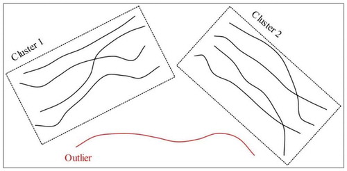
For three main reasons, density-based algorithms are appropriate choices for trajectory clustering. First, in many real-world applications, captured trajectories inevitably contain some noise and outliers, but as they do not affect the total density of the data, density-based clustering will perform more effectively. Second, in many applications such as analysis of the birds’ movement, the forms of clusters do not follow any particular shape. Therefore, using methods such as K-means which are only able to extract clusters with spherical shape will not yield satisfactory results. On the other hand, using density-based methods which are capable of extracting clusters of arbitrary shape is more reasonable. Third, the number of clusters is not usually previously known. Some of the clustering algorithms require the number of clusters as the input parameter, but density-based algorithms do not suffer from this limitation. Figure 2. demonstrate how the DBSCAN algorithm works for trajectory clustering.

Figure.2. DBSCAN algorithm for trajectory clustering.

3.2.1. DBSCAN algorithm

DBSCAN is one of the most used clustering algorithms, which is based on the notion of density (Ester et al. 1996). The algorithm clusters a set of objects in groups where the density of objects is high and recognizes the ones out of the dense area as outliers. These techniques do not require the number of clusters to be given as an input parameter and also do not make any assumptions about the density within the clusters. The basic idea of using DBSCAN for trajectory clustering is that considering a similarity function (such as Euclidean or DTW), each trajectory existing in a cluster should have at least minTr number of trajectories in its neighbourhood within a radius of Eps.

Given the trajectory dataset TD and distance function dis: TD $\times$ TD$\to$ ${\mathrm{R}}_0^{+}$,in the following, we will introduce the definitions involving the basic idea of using DBSCAN in the trajectory clustering task.

• Eps-neighbourhood of trajectory T_i $\in$ TD is defined by ${\mathrm{N}}_{\mathrm{E}\mathrm{p}\mathrm{s}\left({\mathrm{T}}_{\mathrm{i}}\right)}=\left\{{\mathrm{T}}_{\mathrm{j}}\in \mathrm{T}\mathrm{D}|\mathrm{d}\mathrm{i}\mathrm{s}\left({\mathrm{T}}_{\mathrm{i}},{\mathrm{T}}_{\mathrm{j}}\right)\le \mathrm{E}\mathrm{p}\mathrm{s}\right\}$. If Eps-neighbourhood of T_o has at least minTr trajectories, T_o is called a core trajectory.

• T_i is directly density-reachable to T_o with respect to Eps, minTr and DF if T_i $\in$ N_Eps(T_o) and |N_Eps(T_o)| ≥ minTr

• For a given Eps, minTr and DF, trajectory T_p is density-reachable from a trajectory T_q if there exists a series of trajectories T₁, …, T_n, T₁ = T_q, T_n = T_p in the condition that T_k is directly density-reachable to T_k+1.

• Trajectories T_i and T_j are density-connected for a given Eps, minTr and DF, if there is a trajectory T_o such that both T_i and T_j are density-reachable from it.

• A cluster C is a non-empty subset of TD, for every Tp, T_q: if T_p $\in$ C, T_q is density-reachable from Tp then T_q $\in$ C and T_p is density-connected to T_q. A trajectory which is not part of any clusters is defined as an outlier.

3.3. Motivation of using clustering validation indices

In distance-based trajectory clustering, the quality of clustering is generally affected by choice of the Distance Function. It is necessary to assess the efficiency of different DFs for both spatial and spatio-temporal aspects. Different partitions generated by the clustering algorithm from the same data are not equally useful and can sometimes be misleading. Therefore, assessment and validation of the results is a crucial task and at the same time a difficult one. Each clustering method results in a unique grouping of objects and also requires unique computation time. Computation time and clustering quality are among the most frequently used measuring criteria for evaluation of the clustering methods. In case of large high-dimensional datasets like trajectories visual perception of the clusters structure is unable to assess the quality of a clustering, and proper clustering validation indices should be employed.

In general, there are two main approaches to evaluate the clustering results: internal and external criteria. An external validation index uses prior knowledge, whereas an internal index is only based on information from the data. In this paper, we use both internal and external approaches.

3.3.1. External validation measure

External clustering validation approaches compare clustering results with externally given cluster labels. In other words, these indices measure the degree to which cluster labels affirm ground truth. Assume that the trajectory dataset TD, and true clustering classes C = {c₁,c₂, …, c_J} are available. We use Purity as a common external validation index to evaluate clusters Cʹ = {cʹ₁,cʹ₂, …, cʹ_K} as follows:

(13) $\mathrm{P}\mathrm{u}\mathrm{r}\mathrm{i}\mathrm{t}\mathrm{y}\left({\mathrm{C}}^{\prime }\right)=\frac{1}{\mathrm{n}}\sum _{\mathrm{k}}\underset{\mathrm{j}}{max}\left|\mathrm{c}{ }_{\mathrm{k}}^{\prime }\cap {\mathrm{c}}_{\mathrm{j}}\right|$(13)

3.3.2. Internal validation measure

In real-world applications, there are no predefined classes in the clustering process. Consequently, external measures are not practical to determine whether the found cluster has a satisfactory configuration. Internal criteria measure the quality of clustering without any external information using only information intrinsic to the data. Examples include Dunn’s measure (Dunn 1974), Silhouette (Rousseeuw 1987), and Davies-Bouldin’s measures (Davies and Bouldin 1979). However, many of the current validation criteria are developed for the evaluation of convex shaped clusters and have major issues with trajectory clusters which are usually dense and arbitrarily shaped. CS index is a validation measure that can handle this issue and shows superiority to other indices in term of coping with clusters of different densities, sizes, and shapes (RamakrishnaMurty, Murthy, and Prasad Reddy; Chou, Su, and Lai 2004). Having a TD dataset partitioned as C = {C₁,C₂, …, C_K}, CS measure is computed using the following equation:

(14) $\mathrm{C}\mathrm{S}=\frac{{\sum }_{\mathrm{i}=1}^{\mathrm{K}}\left[\frac{1}{\left|{\mathrm{C}}_{\mathrm{i}}\right|}{\sum }_{{\mathrm{T}}_{\mathrm{i}\in }{\mathrm{C}}_{\mathrm{i}}}\underset{{\mathrm{T}}_{\mathrm{q}}\in {\mathrm{C}}_{\mathrm{i}}}{max}\left\{\mathrm{d}\mathrm{i}\mathrm{s}\left({\mathrm{T}}_{\mathrm{i}},{\mathrm{T}}_{\mathrm{q}}\right)\right\}\right]}{{\sum }_{\mathrm{i}=1}^{\mathrm{K}}\left[\underset{\mathrm{j}\in \mathrm{K},\mathrm{j}\ne \mathrm{i}}{min}\left\{\mathrm{d}\mathrm{i}\mathrm{s}\left({\mathrm{R}}_{\mathrm{i}},{\mathrm{R}}_{\mathrm{j}}\right)\right\}\right]}$(14)

where R_i is the representative trajectory for the cluster C_i and dis is the similarity function of the trajectories.

The trajectory clustering aims to describe the trajectory dataset as a group of clusters based on their movement characteristics. The reason for defining different distance functions is the different definitions of similarity in different applications and various aspects of similarity, such as spatial and spatio-temporal. Therefore, in order to address this issue, two spatial and spatio-temporal indicators are applied to evaluate the results more precisely.

3.3.2.1. Spatial

In some applications, in order to extract and discover useful information, it is very limiting to investigate trajectories which have the same path and are captured in a similar time. Spatial similarity only considered spatial closeness of trajectories, and ignore their temporal dimension. Accordingly, it does not address the similarity of movement parameters like velocity and acceleration. In this study, in order to investigate the quality of clustering from the spatial aspect, the Euclidean distance is chosen to be the dis(T_i, T_j) in Equation (14), because it is a fast function and it can also evaluate the spatial closeness of trajectories effectively.

3.3.2.2. Spatio-temporal

The aim of spatio-temporal similarity is considering both the spatial and temporal dimensions of trajectories and their other dynamic characteristics such as velocity (Pelekis et al. 2007). In applications such as smart transportation which is aimed at discovering the pattern of vehicles on the roads, and also the traffic anomaly detection, it is important to pay attention to the density of trajectories and their speed changes. Hence, the quality assessment of clustering result considering only the spatial closeness of trajectories inside clusters is not enough. To evaluate the clustering quality from a spatio-temporal point of view and using CS indicator, we formulate dis(Ti, Tj) in Equation (14) as detailed below:

1. Showing each trajectory T_i as a vector of velocities V_i = {v₁, v₂, …, v_m} such that v_p is the velocity in i ^th point of trajectory T_i.

2. Using linear interpolation to equalize the length of vectors V_i and V_j.

3. Utilizing Euclidean distance to calculate the distance between two velocity borders after equalizing the lengths.

The less the value of Spatial and Spatio-temporal CS, the higher is the quality of the clustering in terms of velocity similarity of cluster members with each other.

4. Implementation and evaluation

In the current paper, the CVRR trajectory Analysis dataset provided by the Computer Vision and Robotics Department of the University of California, San Diego is used for the trajectory clustering task (Morris and Trivedi 2011). It consists of five different simulated scenes, among which i5, cross, and labomni are employed in this study and are illustrated in Figure 3. Their trajectories contain only the spatial information, and velocity must be inferred. I5 is a highway trajectory in both directions including 806 trajectories, cross is a four-way traffic intersection which includes 1900 trajectories, and labomni contains 209 trajectories of humans walking through a lab. In order to properly investigate the clustering performance of different DFs, noise with Gaussian distribution and a Signal-to-Noise Ratio (SNR) of 2 and 5 and outlier data with 1% and 2% have been added to these two datasets. Table 1. summarizes, for each data, important movement parameters.

Figure 3. Trajectory datasets (a) cross, (b) i5, and (c) labomni.

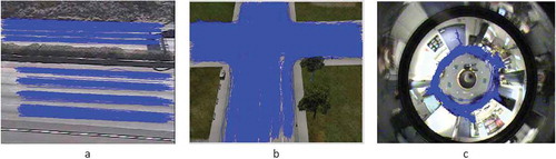
Table 1. The characteristics of the data under study.

Datasets	No. Trajectory	No. Cluster	Speed deviation	Length deviation	Shape complexity
I5	806	8	2.38	4.10	1.00
Cross	1900	19	5.07	4.27	0.85
Labomni	209	15	0.31	142.26	0.71

4.1. Pre-processing

Lengths of trajectories vary significantly, not only because of inconsistent sampling rates but also because of the gap(s) caused by sensor failures. In Euclidian and L1 distances, trajectories are required to be the same length.

Therefore, linear interpolation can be used as the pre-processing operation to transform trajectories to similar lengths. The value of non-acquisition point p at the time t can be estimated by Eq. 18.

(15) $\mathrm{v}\mathrm{a}\mathrm{l}\mathrm{u}\mathrm{e}=\frac{\mathrm{v}\mathrm{a}\mathrm{l}\mathrm{u}{\mathrm{e}}_{\mathrm{p}2}-\mathrm{v}\mathrm{a}\mathrm{l}\mathrm{u}{\mathrm{e}}_{\mathrm{p}1}}{{\mathrm{t}}_2-{\mathrm{t}}_1}\times \left(\mathrm{t}-\mathrm{t}1\right)+\mathrm{v}\mathrm{a}\mathrm{l}\mathrm{u}{\mathrm{e}}_{\mathrm{p}1}$(15)

where p1, p2, t₁, and t₂ are the first point before P, the first point after P, the acquisition time of p1 and acquisition time of p2, respectively.

4.2. Effectiveness of CS measure

In this part, the effectiveness of the proposed indicators for trajectory clustering is investigated. Three different trajectory datasets (Figure 4.) are clustered using the DBSCAN algorithm with the different number of clusters, and the value of Spatial CS in different K’s are shown in Table 2. As it is evident from the table, this indicator has performed successfully in finding the appropriate number of clusters in three cases: clusters with different shapes, clusters with different shapes and sizes, and clusters with different shapes and densities.

Figure 4. Demonstration of trajectories with (a) different shapes (b) different shapes and sizes (c) different shapes and densities.

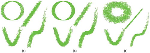
Table 2. Numerical value of spatial CS measure in different cases.

Trajectory cluster types	K = 2	K = 3	K = 4	K = 5	K = 6	K = 7	K = 8
Different shape	2.4387	4.2299	2.0633	4.1786	6.2097	9.6821	13.1705
Different shape and size	2.7544	2.3283	1.4779	2.4174	6.1859	9.8899	14.2855
Different shape and density	2.4795	1.7450	0.7585	6.0539	9.9306	14.3994	19.4300

4.3. Parameter analysis

Despite all the advantages of the DBSCAN algorithm, it suffers from sensitivity to the input parameters. However, without understanding the characteristics of the trajectory dataset, determining an appropriate value for this parameter is a challenging task. For example, with a given minTr, if a low value of Eps is considered, many of the trajectories will be recognized as outliers and on the other hand considering a high value for Eps will result in containing the outliers in the clusters that lead to the integration of small clusters forming big ones. These clustering results might be inappropriate to conclude from about the data. Considering this, we conduct the experiment with different values of Eps and MinTr in order to investigate the input parameter effects on clustering outcomes. In the figure below the values for two spatial and spatio-temporal indicators for different values of Eps and MinTr in the labomni clustering and with EDR distance is shown which can be used to choose appropriate values for these parameters.

4.4. Clustering results

For the purpose of evaluating similarity functions’ performance in density-based trajectory clustering, different DFs, and DBSCAN algorithm are run on a core i5 computer with 8G RAM. Setting the parameters of DBSCAN is one of the challenges of these algorithms. To obtain the desired number of clusters for each dataset, each DF with different values of Eps and MinTr was executed, and the best results were considered in this paper.

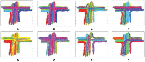
In Figure 6., clustering results for different methods on the cross data are depicted, and each group is shown with a different colour. Trajectories which are assigned to no clusters denote noises and are shown by black circles. Due to the space limitations, i5 and labomni results are not discussed in this paper. It is observed from the figures below that trajectories with the same path are placed in the same group. Clusters with different shape, despite using the same clustering method, shows the effect of the used DF on the geometrical shape of clusters.

Figure 5. Determine the input parameters of DBSCAN algorithm using (a) Spatial CS measure and (b) Spatio-temporal CS measure.

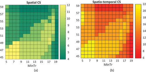
Figure 6. Clustering results with DBSCAN algorithm using (a) Euclidean, (b) L1, (c) Fréchet, (d) Hausdorff, (e) LCSS, (f) DTW, (g) ERP, (h) EDR.

4.4.1 Purity for original data

In Table 3, Purity index for different similarity functions are illustrated. According to the results, for each dataset, a different similarity function has shown the best performance, which indicates the dependence of the optimum similarity function on the data. In i5, Hausdorff distance with the purity index value of 0.6166, in cross, the Euclidean distance with the purity index value of 0.9153 and in labomni, the Fréchet distance with the purity index value of 0.9091 have obtained the most suitable results. Considering all three datasets together, the Euclidean distance with the average value of 0.7447 for purity index has had a stronger performance among the mentioned DFs in density-based clustering of trajectories.

Table 3. Purity value for different distances.

Distance	i5	Cross	Labomni
Euclidean	0.6055	0.9153	0.8708
L1	0.6166	0.9105	0.8469
DTW	0.6663	0.4037	0.5024
Fréchet	0.5112	0.7858	0.9091
Hausdorf	0.7494	0.3579	0.1770
LCSS	0.3052	0.2737	0.3110
EDR	0.3524	0.5711	0.7751
ERP	0.5955	0.5579	0.5167

4.4.2 Purity in the presence of error

Some errors are inevitable in capturing the trajectory points’ locations using measurement devices like GPS. The errors appear as two major forms of noise and outliers. Thus, it is essential to pay attention to these two errors in trajectory clustering. In order to conduct experiments considering the effect of errors on the performance of DFs; at first step, noise with Signal to Noise Ratio of 2 and 5 was added to all three datasets. In Figures 7 and 8, the error percentage resulted from imposing noise and outlier, respectively, on the results in Table 3. is illustrated. According to the results, the noise did not affect the results of L1 and LCSS distances, whereas DTW has been affected the most. Among all three datasets, i5 has been the most sensitive against noise.

Figure 7. Error caused by imposing noise on original data.

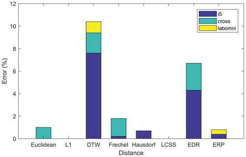
Figure 8. Error caused by imposing noise on original data.

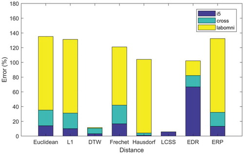
In the next step, 1% and 2% of outliers were added to the three datasets, and the results are shown in Figure 9 As it is observable from this figure, the presence of outliers severely affects the results. Hence, using proper preprocessing techniques to eliminate outliers is necessary. Additionally, because of LCSS distance’s nature, it has shown to be more resistant to outliers than other DFs. The quality of results using LCSS for cross and labomni datasets in case of containing outliers have not changed from than that of containing any outliers. Another surprising point is the low sensitivity of DTW results against outliers, whereas it has been undertaking the most from noise. On the other hand, L1, which had a satisfactory performance in the case of containing noise, showed highly dependent and sensitive to outliers. The main conclusion of the above experiments is that despite the functional abilities of the DBSCAN algorithm in handling noise, it cannot perform satisfactorily against outliers in most DFs. However, LCSS distance has proved to be remarkably resistant to both noise and outliers.

4.4.3. Spatial and spatio-temporal CS

In the following part, a comparison between the similarity functions using indicators which were introduced in section 3.3.2 has been made and discussed. As can be observed from Table 4, in total, EDR has achieved the best results regarding the spatial similarity with the average spatial CS value of 28.50. It means that using this distance in applications in which only the spatial closeness of trajectories is important will be more optimum than other similarity functions. L1, Euclidean, Fréchet, ERP, LCSS, and Hausdorff have achieved the next ranks in the best DFs. On the other hand, considering Spatio-temporal CS measure, EDR again has obtained the best result than other distance with the average spatio-temporal CS value of 40.86. After EDR distance, Fréchet, DTW, LCSS, L1, ERP, and Euclidean distances have shown higher ranks concerning the value of Spatio-temporal CS measure.

Table 4. Numerical value of spatial and spatio-temporal CS measure in different distances.

	I5		CROSS		LABOMNI
Distance	Spatial CS	Spatio-temporal CS	Spatial CS	Spatio-temporal CS	Spatial CS	Spatio-temporal CS
Euclidean	29.01	127.49	61.51	94.94	34.63	37.52
L1	27.97	123.18	50.62	62.67	34.97	37.52
DTW	40.33	67.57	23.02	25.19	99.15	58.11
FRÉCHET	34.12	43.53	61.67	51.94	39.59	43.47
HAUSDORF	58.87	66.70	117.66	64.45	-	-
LCSS	57.81	55.44	164.04	103.63	113.56	42.26
EDR	15.04	42.76	35.75	34.70	34.70	45.13
ERP	41.96	86.09	124.46	133.90	75.12	37.77

Another salient point in Table is that for the cluster members, Euclidean and L1 distances have shown a satisfactory performance regarding the spatial closeness and a weak performance with regard to the spatio-temporal similarity. This denotes that using these DFs can only achieve acceptable results only in cases in which the temporal dimension of trajectories is ignored, and therefore adding time will not yield satisfactory outcomes. By getting along well with the time shift, EDR and Fréchet distances, have obtained the first and the second ranks respectively in density-based trajectory clustering regarding the velocity similarity of cluster members with each other. Taking into account the optimum performance of EDR, the clustering quality in a different number of clusters is depicted in Figure 5.

4.4.4. Computation time

Figure 10 pinpoints the efficiency of different DFs in terms of computation time. As illustrated in this figure, by increasing the data size, the running time of all algorithms is increased. However, this increase is less significant in Euclidean, L1 Norm, and LCSS methods than other methods. This mentions a lower dependence of these methods on the increase of the data volume. By increasing data volume by four times, the running time is multiplied about ten times for Euclidean, L1 Norm, and LCSS and about 17 times for other DFs.

Figure 9. CS measure for different number of clusters.

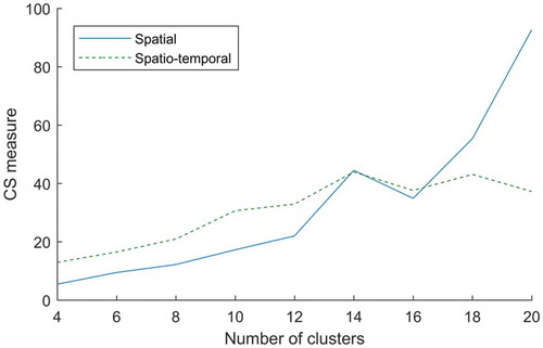
Figure 10. Performance comparison of different distance functions in clustering with the DBSCAN algorithm.

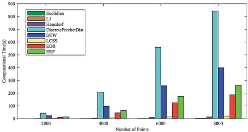
It is observable that the running time of clustering using the Euclidean and L1 Norm is less than 10 seconds, which is insignificant comparing to other methods. The high running time of Fréchet is another critical point in this graph. With a data volume of 2000 points, running time of clustering using Fréchet is 50 seconds, and with increasing the data volume by four times, it will increase to 800 seconds. After Fréchet distance, DTW is proving to be costly and time-consuming.

5. Conclusion

As stated in the introduction, density-based methods are best suited for arbitrarily-formed clusters among the various kinds of existing clustering methods. Therefore, our main objective was to evaluate the effectiveness of well-known Distance Functions in density-based clustering of trajectories from two spatial and spatio-temporal aspects. In this paper, we evaluated the performance of different DFs in the presence of two common types of error (noise and outlier). Choosing an appropriate DF in density-based trajectory clustering is a challenging task, and as can be observed from the experimental results, it depends on both data and movement parameters of. Hence, considering the Purity index, the best three results for i5, cross, and labomni dataset are achieved by Hausdorf, Euclidean, and Fréchet distances, respectively.

Besides, considering the fact that trajectory datasets usually have many noise and outliers. This experiment shows that density-based clustering algorithms are marginally affected by noise regardless of the utilized Distance Function. However, the presence of outliers severely influences the results of most of the DFs. LCSS and in the next rank, DTW have proven to be highly resistant against outliers in the trajectory datasets.

In this experiment, we find that although Lp-norm distances are fast and easy to compute, there are two major problems in utilizing them for density-based clustering of trajectories. First, results achieved from these DFs are highly influenced by the presence of noise and outliers, although L1 is less affected than Euclidean distance. Second, due to not supporting local time shifts, the quality of clustering is deficient from spatio-temporal aspect comparing to the spatial point of view. In order to deal with the first problem, in this study using LCSS distance is suggested for density-based clustering of trajectories. Unlike Lp-norm distance, LCSS permits some elements to remain unmatched. Hence in case of unreliability about the preprocessing procedures using LCSS is recommended. Besides, our experiment states the superiority of LCSS over DTW, ERP, EDR, Fréchet, and Hausdorff distances in terms of computation time and scalability. Despite the ability of this distance function to cope with errors, LCSS is a coarse measure, as it does not differentiate between trajectories in density-based trajectory clustering. As can be seen from the results,it performed poorly in both Purity and CS measures. Different speeds of the moving objects may lead to local time shifts in trajectories. DTW, LCSS, and EDR have been proposed to address this problem. However, in this experiment, we find that despite the promising result of EDR and at the next rank DTW, LCSS could not yield satisfactory results regarding velocity similarity of cluster members. After EDR, Fréchet distance has obtained one of the best performances due to the consideration of the order of points in trajectories besides their geometry. As can be seen from Table 3, Fréchet has performed more satisfactorily in labomni than the other two datasets because of its complexity of data.

We propose that further research investigate the effect of geometrical transformations, changes in the acquisition rate of the points, and time shift on the performance of different DFs. Moreover, depending on the intended application, it is possible to benefit from different data with more different characteristics than the data used in this study.

Disclosure statement

No potential conflict of interest was reported by the authors.

References

- Aghabozorgi, S., A. S. Shirkhorshidi, and T. Y. Wah. 2015. “Time-series clustering–A Decade Review.” Information Systems 53: 16–38. doi:10.1016/j.is.2015.04.007.
- Ali Abbaspour, R., M. Shaeri, and A. Chehreghan. 2017. “A Method for Similarity Measurement in Spatial Trajectories.” Spatial Information Research 25 (3): 491–500. doi:10.1007/s41324-017-0115-5.
- Alt, H., and M. Godau. 1995. “Computing the Fréchet Distance between Two Polygonal Curves.” International Journal of Computational Geometry & Applications 5 (01n02): 75–91. doi:10.1142/S0218195995000064.
- Andrienko, G., and N. Andrienko. 2010. “Interactive Cluster Analysis of Diverse Types of Spatiotemporal Data.” Acm Sigkdd Explorations Newsletter 11 (2): 19–28. doi:10.1145/1809400.
- Atev, S., G. Miller, and N. P. Papanikolopoulos. 2010. “Clustering of Vehicle Trajectories.” IEEE Transactions on Intelligent Transportation Systems 11 (3): 647–657. doi:10.1109/TITS.2010.2048101.
- Basiri, A., P. Amirian, and P. Mooney. 2016. “Using Crowdsourced Trajectories for Automated OSM Data Entry Approach.” Sensors 16 (9): 1510. doi:10.3390/s16122100.
- Berkhin, P. 2006. “A Survey of Clustering Data Mining Techniques.” In: Kogan J., Nicholas C., Teboulle M. (eds)., Grouping Multidimensional Data, 25–71. Springer, Berlin: Springer.
- Berndt, D. J., and J. Clifford. 1994. “Using Dynamic Time Warping to Find Patterns in Time Series.” Paper presented at the KDD workshop.
- Besse, P., B. Guillouet, J.-M. Loubes, and F. Royer. 2015. “Review and Perspective for Distance Based Trajectory Clustering.” ARXIV.
- Besse, P. C., B. Guillouet, J.-M. Loubes, and F. Royer. 2016. “Review and Perspective for Distance-based Clustering of Vehicle Trajectories.” IEEE Transactions on Intelligent Transportation Systems 17 (11): 3306–3317. doi:10.1109/TITS.2016.2547641.
- Birant, D., and A. Kut. 2007. “ST-DBSCAN: An Algorithm for Clustering Spatial–Temporal Data.” Data & Knowledge Engineering 60 (1): 208–221. doi:10.1016/j.datak.2006.01.013.
- Chen, J., R. Wang, L. Liu, and J. Song. 2011a. “Clustering of Trajectories Based on Hausdorff Distance.” Paper presented at the Electronics, Communications and Control (ICECC), 2011 International Conference on Ningbo, China.
- Chen, J., R. Wang, L. Liu, and J. Song. 2011b. “Clustering of Trajectories Based on Hausdorff Distance.” Paper presented at the 2011 International Conference on Electronics, Communications and Control (ICECC), Ningbo, China.
- Chen, L., M. Tamer Özsu, and V. Oria. 2005. “Robust and Fast Similarity Search for Moving Object Trajectories.” Paper presented at the Proceedings of the 2005 ACM SIGMOD international conference on Management of data, New York, USA.
- Cheng, Z., L. Jiang, D. Liu, and Z. Zheng. 2018. “Density Based Spatio-temporal Trajectory Clustering Algorithm.” Paper presented at the IGARSS 2018-2018 IEEE International Geoscience and Remote Sensing Symposium Valencia.
- Chou, C.-H., M.-C. Su, and E. Lai. 2004. “A New Cluster Validity Measure and Its Application to Image Compression.” Pattern Analysis and Applications 7 (2): 205–220. doi:10.1007/s10044-004-0218-1.
- Clarke, F. H. 1976. “Optimal Solutions to Differential Inclusions.” Journal of Optimization Theory and Applications 19 (3): 469–478. doi:10.1007/BF00941488.
- Davies, D. L., and D. W. Bouldin. 1979. “A Cluster Separation Measure.” IEEE Transactions on Pattern Analysis and Machine Intelligence PAMI-1 (2): 224–227. doi:10.1109/TPAMI.1979.4766909.
- Dunn, J. C. 1974. “Well-separated Clusters and Optimal Fuzzy Partitions.” Journal of Cybernetics 4 (1): 95–104. doi:10.1080/01969727408546059.
- Ester, M., H.-P. Kriegel, J. Sander, and X. Xiaowei 1996. “A Density-based Algorithm for Discovering Clusters in Large Spatial Databases with Noise.” Paper presented at the Kdd HINNEBURG.
- Georgiou, H., S. Karagiorgou, Y. Kontoulis, N. Pelekis, P. Petrou, D. Scarlatti, and Y. Theodoridis. 2018. “Moving Objects Analytics: Survey on Future Location & Trajectory Prediction Methods.” arXiv Preprint arXiv:1807.04639.
- Han, J., J. Pei, and M. Kamber. 2011. Data Mining: Concepts and Techniques. Elsevier.
- Jajuga, K. 1987. “A Clustering Method Based on the L1-norm.” Computational Statistics & Data Analysis 5 (4): 357–371. doi:10.1016/0167-9473(87)90058-2.
- Kearney, J. K., and S. Hansen. 1990. Stream Editing for Animation. Department of Computer Science University of Iowa.
- Khoshaein, V. 2013. “Trajectory Clustering Using a Variation of Fréchet Distance.” (Doctoral dissertation, University of Ottawa). Citeseer.
- Kriegel, H., P. Kröger, J. Sander, and A. Zimek. 2011. “Density‐based Clustering.” Wiley Interdisciplinary Reviews: Data Mining and Knowledge Discovery 1 (3): 231–240.
- Kruskal, J. B. 1983. “An Overview of Sequence Comparison: Time Warps, String Edits, and Macromolecules.” SIAM Review 25 (2): 201–237. doi:10.1137/1025045.
- Lee, J.-G., J. Han, and K.-Y. Whang. 2007. “Trajectory Clustering: A Partition-and-group Framework.” Paper presented at the Proceedings of the 2007 ACM SIGMOD international conference on Management of data.
- Mahdavinejad, M. S., M. Rezvan, M. Barekatain, P. Adibi, P. Barnaghi, and A. P. Sheth. 2018. “Machine Learning for Internet of Things Data Analysis: A Survey.” Digital Communications and Networks 4 (3): 161–175. doi:10.1016/j.dcan.2017.10.002.
- Morris, B. T., and M. M. Trivedi. 2011. “Trajectory Learning for Activity Understanding: Unsupervised, Multilevel, and Long-term Adaptive Approach.” IEEE Transactions on Pattern Analysis and Machine Intelligence 33 (11): 2287–2301. doi:10.1109/TPAMI.2011.64.
- Myers, C., L. Rabiner, and A. Rosenberg. 1980. “Performance Tradeoffs in Dynamic Time Warping Algorithms for Isolated Word Recognition.” IEEE Transactions on Acoustics, Speech, and Signal Processing 28 (6): 623–635. doi:10.1109/TASSP.1980.1163491.
- Pelekis, N., I. Kopanakis, G. Marketos, I. Ntoutsi, G. Andrienko, and Y. Theodoridis. 2007. “Similarity Search in Trajectory Databases.” Paper presented at the 14th International Symposium on Temporal Representation and Reasoning (TIME’07).
- Pfeifer, P. E., and S. J. Deutrch. 1980. “A Three-stage Iterative Procedure for Space-time Modeling Phillip.” Technometrics 22 (1): 35–47. doi:10.2307/1268381.
- Picton, T., M. Hunt, R. Mowrey, R. Rodriguez, and J. Maru. 1988. “Evaluation of Brain-stem Auditory Evoked Potentials Using Dynamic Time Warping.” Electroencephalography and Clinical Neurophysiology/Evoked Potentials Section 71 (3): 212–225. doi:10.1016/0168-5597(88)90006-8.
- Priestley, M. B. 1980. “State‐dependent Models: A General Approach to Non‐linear Time Series Analysis.” Journal of Time Series Analysis 1 (1): 47–71. doi:10.1111/j.1467-9892.1980.tb00300.x.
- Ranacher, P., and K. Tzavella. 2014. “How to Compare Movement? A Review of Physical Movement Similarity Measures in Geographic Information Science and Beyond.” Cartography and Geographic Information Science 41 (3): 286–307. doi:10.1080/15230406.2014.890071.
- Richalet, J., A. Rault, J. L. Testud, and J. Papon. 1978. “Model Predictive Heuristic Control.” Automatica (journal of IFAC) 14 (5): 413–428. doi:10.1016/0005-1098(78)90001-8.
- Rick, C. 2000. “Efficient Computation of All Longest Common Subsequences.” Paper presented at the Scandinavian Workshop on Algorithm Theory. Berlin, Heidelberg: Springer.
- Rousseeuw, P. J. 1987. “Silhouettes: A Graphical Aid to the Interpretation and Validation of Cluster Analysis.” Journal of Computational and Applied Mathematics 20: 53–65. doi:10.1016/0377-0427(87)90125-7.
- Takens, F. 1980. “Motion under the Influence of a Strong Constraining Force.” In Global Theory of Dynamical Systems, 425–445. Berlin, Heidelberg: Springer.
- Vlachos, M., G. Kollios, and D. Gunopulos. 2002a. “Discovering Similar Multidimensional Trajectories.” Paper presented at the Data Engineering, 2002. Proceedings. 18th International Conference on data engineering, San Jose, CA, USA, USA..
- Vlachos, M., G. Kollios, and D. Gunopulos. 2002b. “Discovering Similar Multidimensional Trajectories.” Paper presented at the Proceedings 18th international conference on data engineering, San Jose, CA, USA.
- Wang, H., S. Han, K. Zheng, S. Sadiq, and X. Zhou. 2013. “An Effectiveness Study on Trajectory Similarity Measures.” Paper presented at the Proceedings of the Twenty-Fourth Australasian Database Conference-Volume, 137, Adelaide, Australia.
- Wei, L.-X., X.-H. He, Q.-Z. Teng, and M.-L. Gao. 2013. “Trajectory Classification Based on Hausdorff Distance and Longest Common Subsequence.” Dianzi Yu Xinxi Xuebao(Journal of Electronics and Information Technology) 35 (4): 784–790.
- Xu, R., and D. Wunsch. 2005. “Survey of Clustering Algorithms.” IEEE Transactions on Neural Networks 16 (3): 645–678. doi:10.1109/TNN.2005.845141.
- Yuan, G., P. Sun, J. Zhao, L. Daxing, and C. Wang. 2017. “A Review of Moving Object Trajectory Clustering Algorithms.” Artificial Intelligence Review 47 (1): 123–144. doi:10.1007/s10462-016-9477-7.
- Zhang, X., H. Liu, X. Zhang, and X. Liu. 2014. “Novel Density-Based Clustering Algorithms for Uncertain Data.” Neural Networks 93 (2017): 240-255.
- Zhao, L., and G. Shi. 2019. “A Trajectory Clustering Method Based on Douglas-Peucker Compression and Density for Marine Traffic Pattern Recognition.” Ocean Engineering 172: 456–467. doi:10.1016/j.oceaneng.2018.12.019.
- Zheng, Y., L. Zhang, X. Xie, and M. Wei-Ying. 2009. “Mining Interesting Locations and Travel Sequences from GPS Trajectories.” Paper presented at the Proceedings of the 18th international conference on World wide web, Madrid, Spain.