GIS-based multi criteria decision making method to identify potential runoff storage zones within watershed

ABSTRACT

The objective of this study was to identify potential runoff storage zones based on the various physical characteristics of the Vishwamitri watershed using a GIS-based conceptual framework that combines through analytic hierarchy process using multi criteria decision-making method. The conceptual framework will help to identify potential runoff storage zones for water storage sites based on the various physical characteristics (rainfall, slope, land use/land cover, height above the nearest drainage, stream order, curve number, topographic wetness index) of the watershed. It was found out that 17% of the area is optimally suitable, 33.2% of the area is moderately suitable, 33.1% of the area is marginally suitable and 18.7% of the area is not suitable for water storage zones/structures. Results will help concerned authorities in the proficient arrangement and execution of water-related plans and schemes, improve water shortage, reduce dependability on ground water and ensure sustainable water availability for local and agricultural purposes in the study area.

KEYWORDS:

• Analytic Hierarchy Process (AHP)
• Multi Criteria Decision-Making (MCDM)
• GIS
• runoff
• water storage

1. Introduction

A naturally occurring geohydrological unit draining to a common point by a system of natural streams/drains is defined as a watershed. The integrated watershed management is a multidisciplinary approach for rational utilization of natural resources existing in the watershed. The existing water resources of most of the countries are underneath the growing pressure of population and rapidly growing urban areas that results in the water deficiency and food insecurity. Potential runoff storage zones in a catchment are the zones where rainwater-harvesting structures like small dams or check dams, nala bunds, gully plug, bundhis (local name in India), percolation tanks etc. can be constructed in a planned and systematic manner to create water buffer within the catchment, which will help reducing vulnerability to drought and seasonal variations in rainfall. These structures can be used for multiple purposes, such as agriculture, livestock watering and domestic use. In general, check dams are constructed at lower order streams, the slope of the terrain should be from flat to gentle so as to retain maximum quantity of water with less height of check dam. It should be located nearer to agricultural areas and settlement to convey the water. Check dams have greater importance than other structures since it has got a complimentary benefit of controlling soil erosion. Nala bunds and percolation tanks are structures constructed across or nearer to nalas (streams) for checking velocity of runoff, increasing water percolation, increasing soil moisture regime and to hold the silt flow, which would otherwise reach the multipurpose reservoirs and reduce their useful life. Nala bunds are less expensive, smaller in dimension and constructed using locally available material whereas, percolation tanks are larger and more expensive than nala bunds. The feasibility of site for locating percolation tanks depends upon technical and economic considerations such as, the sites should be selected in a relatively flat nala reach and the slope of the nala should preferably not be more than 2 percent. Water harvesting bundhis are almost similar to the minor irrigation tanks except that they do not have extensive canal system and their command area is limited to the fields of downstream. It is used to collect and impound surface runoff during monsoon rains and facilitate infiltration to raise groundwater level in the zone of influence of the bundhi. It provides irrigation in the fields lying in close proximity of the water harvesting bundhi. It also moderates the peak flow, partly by storing and partly through flooding.

Water scarcity has become serious problem in several parts of the world, especially in developing nations like India Kumar and Jhariya (2017). In India, ever-increasing population exerts enormous pressure on the water resources of the country due to which per capita water availability is decreasing day by day Singh, Jha, and Chowdary (2017). There is a growing need for cost effective and time saving methods to identify areas that are suitable for water storage. Hence, it becomes necessary to tap the maximum possible water within the watershed. Before execution water storage structures require significant investment and hence it is important to identify the potential runoff storage zones for these structures. Remote sensing (RS) and Geographic information systems (GISs) together fulfil this need by providing a conceptual framework for collecting and analysing spatial and non-spatial data (Krois and Schulte (2014)). Proper selection of factors is of great importance for identifying sites for specific water storage structures. A review of the literature done by Ammar et al. (2016) found that a different number of layers have been used by researchers to rely on the availability of data for potential water storage areas or to identify sites suitable for rainwater harvesting. In several studies related to the identification of water storage sites, the weighted linear combination technique has been used for the integration of biophysical layers in a GIS environment. Weerasinghe, Schneider, and Loew (2011) focused on using a GIS and RS and developed a spatial analysis model named Geographic Water and Management Potential. The model was able to find potential water harvesting and storage sites for water storage and soil-moisture conservation on farms. In most studies, range of weights was decided arbitrarily or weights were assigned on the scale of 1–5 or 1–100, whereas only a few studies assigned weights on the standard 1–9 scale, as suggested by Saaty (1987). De Winnaar, Jewitt, and Horan (2007) conducted a study in which the SCS-CN method was applied to identify potential runoff-harvesting sites in a small sub-catchment in South Africa. The input data included socio-economic data gathered from available data and from field surveys, a digital elevation model (DEM) with 20-m resolution to extract slope information, a soil survey provided soil data, digital images and aerial photographs. Similarly, Ghani et al. (2013) explored potential rainwater storage sites by examining runoff patterns using a hydrologic model with the GIS/RS approach. A 90 metre DEM was used as a source for catchment elevation data to determine flow direction, drainage lines and runoff.

Krois and Schulte (2014) presented GIS and multi criteria evaluation approach to identify and rank sites for the implementation of soil and water conservation techniques within the Ronquillo watershed. Criteria maps were created by reclassifying the spatial maps based on the suitability level for each RWH technique. Pairwise comparison matrix method (analytic hierarchy process (AHP)), calculated the relative-importance weight of each criterion for each rainwater harvesting technique. The weighted overlay process (WOP) in GIS determined the suitability maps for each rainwater harvesting technique. Rainfall, runoff coefficient, slope, land use, soil texture and soil depth were selected based on the FAO guidelines. The assessment of the dominance of one criterion over another was based on the authors’ expertise and a literature survey.

A number of studies have been reported for site suitability using Multi Criteria Decision-Making (MCDM) and AHP in GIS environment (Al-Adamat (2008); Pauw, Oweis, and Youssef (2008); Kahinda et al. (2008); Mahmoud and Alazba (2014)). AHP is a popular weighting method in the field of MCDM (Saaty (1977); Rozos, Bathrellos, and Skillodimou (2011); Karimi and Zeinivand (2019)). The AHP is a theory of measurement through a pairwise comparison matrix and relies on the judgements of experts to derive priority scales. It is used as higher cognitive process tool to determine the percentage importance of various criteria used in the determination of suitable sites. The AHP method consists of three main phases: construction of hierarchy, priority analysis of data and confirmation of consistency.

According to the review study done by Ammar et al. (2016) on identification of suitable sites for water storage in arid and semi-arid regions, it was found out that the most common biophysical layers or criteria applied were slope followed by land use/land cover and soil type. We aim to improve the existing methodology by introducing new layers along with the commonly used biophysical layers for estimation of potential runoff storage zones to identify water storage sites.

In the present study, a GIS-based conceptual framework is applied with MCDM technique using AHP to produce suitability map of potential runoff storage zones within the watershed. The conceptual framework will help to identify potential runoff storage zones for water storage sites based on the various physical characteristics (Rainfall, Slope, Land use/land cover, Height above the nearest drainage, Stream order, Curve number (CN), Topographic wetness index (TWI)) of the Vishwamitri watershed. This will help concerned authorities in the proficient arranging and execution of water-related plans and schemes, improve water shortage, reduce dependability on ground water and ensure sustainable water availability for local and agricultural purposes in the study area.

2. Study area

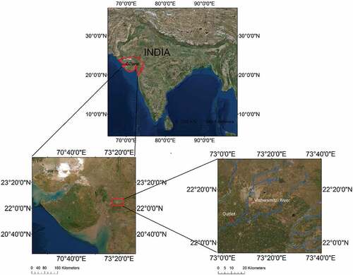
The present study was conducted in the Vishwamitri Watershed in Vadodara district, Gujarat. Vadodara district is located at the south of the Tropic of Cancer in the transition zone of heavy rainfall areas of South Gujarat and arid areas of North Gujarat plains. It has a subtropical climate with moderate humidity and forms a part of the great Gujarat plain. The eastern portion of the district is hilly terrain with several ridges, plateaus and isolated relict hills with an elevation of 150–481 m above the mean sea level. The Vishwamitri river originates from the hills of Pavagadh, 43 km northeast of Vadodara. The Pavagadh hill is made of trappean rocks that emerge abruptly 830 m above the mean sea level. The Viswamitri river has a channel length of around 70 km, of which, 58 km flows through Vadodara district. It meets the Dhadhar river at Pingalwada in Vadodara district. Figure 1 shows the geographical location of the study area.

Figure 1. Geographical location of the study area.

3. Methodology

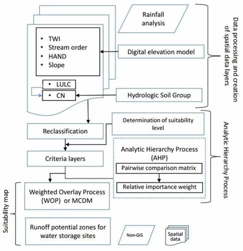
To find the potential runoff storage zones, workflow was divided into four steps (Figure 2). Firstly, the rainfall analysis was carried out using SPI and annual rainfall. Secondly, processing of spatial data and creation of spatial data layers was performed. Thirdly, criteria weights were determined using AHP. Lastly, executing WOP within GIS.

Figure 2. Multi Criteria Decision-Making (MCDM) technique workflow using AHP for identification of potential runoff storage zones for water storage.

3.1. Rainfall analysis

Study area falls under the arid areas of north Gujarat Plains. Potential runoff storage zones or structures require considerable rainfall and hence it is important to analyse variability of rainfall within the watershed for the suitable locations of these storage zones or structures before execution. For rainfall variability analysis two indicators, viz., annual rainfall and Standardized Precipitation Index (SPI) have been used. Annual rainfall is highly influenced by the amount of the rainfall, intensity of the rainfall, frequency of occurrence of the rainfall and distribution over area as well as time of the rainfall. The approach examines the annual rainfall along with the SPI drought index application for Vishwamitri watershed, and it is calculated accordingly by historical precipitation data. Results of SPI and annual rainfall help in evaluating the area whether it is suitable for water storage structures or not. Favourable results qualify the area for identification of suitable sites for water storage.

The SPI calculation for any location is based on the long-term precipitation record for a desired period. Precipitation is normalized using a probability distribution function and allows for the estimation of both dry and wet periods. Daily rainfall data was collected from State Water Data Centre, Gandhinagar, Gujarat. A total of 56 years (1961 to 2016) rainfall data of four rain gauge stations namely Vadodara, Padra, Savli and Waghodia were used for computation of SPI and annual rainfall. Annual SPI classification system used by McKee, Doesken, and Kleist (1993) shown in the Table 1 and it was computed as described by Akinsanola and Ogunjobi (2014) and Adegoke and Sojobi (2015). Positive SPI values indicate greater than median precipitation and negative values indicate less than median precipitation. Drought starts when the SPI value is equal or below −1.0 and ends when the value becomes positive.

Table 1. Annual standardized precipitation index given by McKee, Doesken, and Kleist (1993).

Classification	SPI
Near normal	−0.99 to 0.99
Moderately wet years	1.0 to 1.49
Moderately dry years	−1.0 to −1.49
Very wet	1.5 –to 1.99
Severely dry years	−1.5 to −1.99
Wet extreme	≥ +2.0
Dry extreme	≤ −2.0

= rainfall in each particular year

= mean rainfall in each particular year

= the standard deviation of rainfall in each particular year

3.2. Processing and creation of spatial data layers

3.2.1. Topographic Wetness Index (TWI)

The TWI was first introduced by Beven and Kirkby (1979). TWI is widely used topographically based soil wetness model that identifies wet areas. It is based on the assumption that local topography controls the movement of water in slopped terrain, which quantifies the effect of the local topography on runoff generation. The index is represented as the natural logarithm of the ratio of upslope flow accumulation area and slope at the cell.

Topographic wetness at a particular point on the landscape is the ratio between the catchment area contributing to that point and the slope at that point (Wilson and Gallant 2000). Locations with a high TWI value have large upslope area and are expected to have higher water availability. On the other hand, locations with small TWI value have small upslope area that are assumed to have lower water availability. Also, Steep locations receive a small TWI value and are expected to be better drained than gently sloped locations, which receive a high TWI value Sørensen and Seibert (2007); Hojati and Mokarram (2016); Bjelanovic (2016); Ågren et al. (2014); Loritz et al. (2019).

The TWI calculation for this study was conducted with the use of Topography Toolbox for ArcGIS 10.1 (Dilts 2015). Firstly, the DEM was pre-processed in order to remove shallow sinks, thus an impact of model artefacts in further analysis could be reduced. The second step included calculation of prerequisites for further TWI computation slope and catchment area; the latter parameter was calculated using the Multiple Flow Direction method (Quinn et al. 1991).

3.2.2. Generation of slope map using Topography Position Index (TPI)

The TPI is the basis of the landform classification system. Gallant and Wilson (2000) defined TPI as the relative topographic position of the central point as the difference between the elevation at this point and the mean elevation within a predetermined neighbourhood. Using TPI, landscapes can be classified in slope position classes. Many researchers have used this index in the field of geomorphology (Tagil and Jenness (2008); Liu et al. (2009); McGarigal, Tagil, and Cushman (2009)); geology (Mora-Vallejo et al. (2008); Deumlich, Schmidt, and Sommer (2010); Illés, Kovács, and Heil (2011)); hydrology (Lesschen et al. (2007); Francés and Lubczynski (2011); Liu et al. (2011)); agricultural science (Pracilio et al. (2006)); archaeology (Patterson (2008); Berking, Beckers, and Schütt (2010)).

The TPI is the difference of a cell elevation in a DEM from the mean elevation () of a user specified neighbourhood surrounding. Local mean elevation is subtracted from the elevation value at centre of the local window Gallant and Wilson, (2000) . The range of TPI depends not only on elevation differences but also on the adopted local window. Large local window values mainly reveal major landscape units, while smaller values highlight smaller features, such as minor valleys and ridges.

Where,

= elevation at the central point

= average elevation around the central point within the local window

= total number of surrounding points employed in the evaluation

TPI variation is shown in Figure 3 for arbitrary point elevations (A and B) in a DEM to the mean elevation of a specified neighbourhood around these point elevations. A small neighbourhood consisting of 33 × 33 cell units rectangular window was used in order to identify complex landscape features. The TPI provides a concise and effective technique of landscape classification in accordance with morphology. A higher degree of slope results in a higher run-off potential and low infiltration and a lower degree of slope favours the retention of water and the drainage in the depth. There are a wide range of geomorphological methods and algorithms classify the landscape into morphological classes Burrough, van Gaans, and MacMillan (2000); Deng (2007); Iwahashi and Pike (2007); Hengl and Reuter (2008). Weiss (2001) and Jenness (2006) recommend (Table 2) standard deviations () away from the mean TPI raster as threshold values for classifying six slope positions:

Figure 3. TPI variation is shown for arbitrary point elevations (A and B) in a DEM to the mean elevation of a specified neighbourhood around these point elevations.

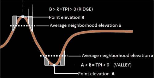
Table 2. Recommend standard deviations (σ) away from the mean TPI raster as threshold values for classifying six slope positions.

Class	Description Breakpoints
Valley	TPI ≤ −1
Lower Slope	−1 < TPI ≤ −0.5
Flat Slope	−0.5 < TPI < 0.5 , Slope ≤ 5°
Middle Slope	−0.5 < TPI < 0.5 , Slope > 5°
Upper Slope	0.5 < TPI ≤ 1
Ridge	TPI > 1

3.2.3. Land use/land cover

Land use pattern of any watershed influences the runoff. To compute hydrological elements more accurately more accurate LULC map is required. By image-processing techniques, image can be produced, which depict some of the characteristics, notably the cover types such as areas with vegetation, water bodies, bare soils etc. The LULC pattern and rainfall have a significant influence on the hydrological response of the watershed.

The Sentinel–2 Level 1 C data product (L1 C_T43QCE_A008039_20180920T054434) acquired on 20 September 2018 was downloaded from the Sentinel Hub developed by European Space Agency. Sentinel–2 Level 1 C data were processed from Top-of-Atmosphere Level 1C to Bottom-Of-Atmosphere Level 2A. The support vector machine classifiers was later used with principal components of sentinel-2 bands for classifying the data into seven major land use and land cover classes namely water, built-up, mixed forest, cultivated land, barren land, fallow land with vertisols dominance and fallow land with inceptisols dominance for the Vishwamitri watershed.

The accuracy assessment was done by comparing the real extent of the classes in the classified image relative to the reference data set using error matrix, which is used to define the quality of the map derived from the data. Accordingly, overall accuracy, producer’s and user’s accuracies and Kappa coefficient were computed. The accuracy and quality of the reference data should be at least one order better as compared to the data to be evaluated. DigitalGlobe’s WorldView-4 data (Product Id: 1ba34688-3ee0-41e4-9187-de68fdb075df-inv) acquired on 25-10-2018 at 5:30 am with 31 cm resolution was used for the accuracy assessment.

The error matrix is represented by a table that shows correspondence between the classification result and a reference image assigned to a particular category, which is relative to the actual category as indicated by the reference data. Producer’s accuracy is the probability that value in a given class was correctly classified (Rana and Suryanarayana (2019b)).

User’s accuracy is the probability that a value predicted to be in a certain class is really in that class.

The kappa coefficient measures the agreement between classification and truth-values. A kappa value of 1 represents perfect agreement, while a value of 0 represents no agreement.

The overall accuracy is given by the ratio of the proportion of the correctly classified pixels to the total number of pixels in the confusion matrix.

3.2.4. Soil texture

Soil texture refers to the relative proportion of clay, silt and sand. Soils containing large proportions of sand have relatively large pores through which water can drain freely. These soils produce less runoff. As the proportion of clay increases, the size of the pore space decreases. This restricts movement of water through the soil and increases the runoff.

Soil data based on soil texture collected from National Bureau of Soil Survey and Land Use Planning (NBSS & LUP). The land use and land cover maps were later used in Hydrologic Engineering Centre’s Geospatial Hydrologic Modelling Extension (HEC-GeoHMS) for the integration of land use land cover and soil data for CN grid preparation. The HEC-GeoHMS is extension to ESRI’s ArcGIS software that compute the Curve Number and other loss rate parameters based on various soil and land use and land cover databases.

3.2.5. Curve Number (CN)

The CN is most commonly used reliable and conceptual technique for estimating surface runoff. CN is basically a dimensionless number that reduces the rainfall to runoff. It depends upon two parameter LULC and Hydrologic Soil Group (HSG). HSG is one of the important parameters for assigning CNs and is generated by reclassifying the soil textural map considering their runoff potential into account (Singh, Jha, and Chowdary (2017); Rizeei, Pradhan, and Saharkhiz (2018); Tripathi (2018)).

The CN grid is a raster containing CN values assigned to each grid cell of land use and land cover and soil complex to indicate their specific runoff potential. A logical condition was defined in ArcGIS to generate the CN raster file from the raster files of Hydrologic Soil Group (HSG) and land use and land cover using TR-55 table Feldman (2000). CNs vary from 0 to 100 and express the runoff response to a given rainfall event. Higher CNs indicate a greater proportion of rainfall to be transformed into surface runoff. Selected CN values for the study area is given in Table 3.

Table 3. Selected curve number values for the study area using TR-55 table.

LULC	Sub classes of LULC	HSG-A	HSG-B	HSG-C	HSG-D
Water	Water	100	100	100	100
Cultivated land	Cultivated land crop1	64	75	82	85
	Cultivated land crop 2	71	80	87	90
Sparsely vegetated	Sparsely vegetated	74	83	88	90
Barren land	Barren land	77	86	91	94
Fallow land (Vertisols dominance)	Fallow land 1 Vertisols dominated	76	85	90	93
	Fallow land 2 Vertisols dominated	76	85	90	93
Fallow land (Inseptisol dominance)	Fallow land 1 inseptisol dominated	74	83	88	90
	Fallow land 2 inseptisol dominated	74	83	88	90
Mixed forest	Mixed forest	36	60	73	79
Builtup	Builtup	89	92	94	95
	Mixed builtup 1	83	89	92	93
	Mixed builtup 2	89	92	98	98

3.2.6. Stream order

The availability of the total quantity of surface water is proportional to the stream order and some particular structure are suitable at a particular drainage order only, for example, check dams should be constructed at lower order streams only (IMSD (1995) and Durga Rao and Bhaumik (2003)).

The stream order of the Vishwamitri watershed was assigned using the Strahler (1957) method. In the Strahler method, all streams without any tributaries are assigned an order of 1 and are referred to as first order. The stream segments starting from the confluence of two streams of the first order are called streams of second order and so on. The tail point of each stream is defined as the point from where a stream of higher order starts. Flow accumulation and flow direction rasters were used to generate stream network using hydrology toolset of ArcGIS. Stream ordering was done for proper planning of conservation measures in terms of storage and capacity.

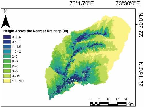
3.2.7. Height above nearest drainage (HAND)

The Height above the nearest drainage is a DEM normalized using the nearest drainage. It normalizes topography according to the local relative heights found along the drainage network and in this way presents the topology of the relative soil gravitational potential, or local draining potentials. HAND allows for the calculation of the elevation of each point in the catchment above the nearest stream it drains to, following the flow direction (Hamdani and Baali (2019); Rennó et al. (2008); Nobre et al. (2011)).

HAND raster was prepared for the 4th and 5th order streams of Vishwamitri watershed as they are highly susceptible to flooding. The first step in generating HAND raster is to remove small imperfection by filling sinks in the Cartosat-1 DEM. Sinks must be filled to ensure a proper delineation of streams. A derived drainage network may be discontinuous if the sinks are not filled Rana and Suryanarayana (2019a). Second step is to create flow-direction raster, it is computed from the DEM using the D8 method (Jenson and Domingue 1988) to determine the flow from each cell to its steepest downslope neighbour. An erroneous flow-direction raster may be resulted in the presence of sinks. Next, the accumulated flow direction is used to find the nearest stream cell for each cell. At last, the elevation of the nearest stream cell is deducted from the elevation of each cell to normalize the terrain and to get its corresponding HAND value.

3.3. Determining criteria weights using AHP

AHP is one of MCDM method that was originally developed by Saaty (1987), it has been widely applied to solve decision-making problems related to water resources. The approach combines mathematics and psychology in dealing with complex decision and in turn converts it into a simpler system of hierarchy. This method compares two criteria at a time through a pairwise comparison matrix, each criterion is assessed by arranging every possible pairing on a ratio scale to express the comparative importance by numerical values. Numerical expression of suitability rating Burnside, Smith, and Waite (2002) and scaling of comparative importance Saaty (1990) is given in Table 4. The judgement on dominance of one criterion over another is based on the authors expertise and a literature survey (Krois and Schulte (2014); Singh, Jha, and Chowdary (2017); Jha et al. (2014); Ammar et al. (2016); Wu, Molina, and Hussain (2018); Prasad, Bhalla, and Palria (2014); Bitterman et al. (2016);).

Table 4. Pairwise comparison scale for AHP preferences.

Numerical expression	Suitability rating	Comparative importance
1	Not suitable	Equal importance
3	Marginally suitable	Moderate importance of one over another
5	Moderately suitable	Essential or strong importance
7	Highly suitable	Very strong importance
9	Optimally suitable	Extreme importance
2, 4, 6, 8	Intermediate values between the two adjacent judgements
Reciprocal of above numbers	If one criterion has one of the above numbers assigned to it when compared with a second criterion, then the second criterion has the reciprocal value when compared to the first.

The determination of the relative importance weight of each criterion (Slope, TWI, LULC, CN, Stream Order and HAND) for potential runoff storage zones is calculated by using the pair-wise comparison matrix method. The number of comparison can be determined using:

where, n = number of criterion

The resulting pair-wise comparison matrix is used to obtain the Eigen value of each criterion, which represents its relative importance weight (Saaty 1990). The relative importance weight given to the criteria one over another is acceptable if the consistency ratio (CR) is less than 10%. If it increases 10%, a new value is assigned in the pair-wise comparison matrix. CR is computed as:

where is principal eigen value, n is the number of elements compared and RI is the so-called random consistency index, a value that depends on the number of criterion that are being compared (Saaty (1987)).

3.4. WOP within GIS

After calculating weights for each criterion, the WOP is applied to construct suitability map, also known as MCDM within a GIS environment. ArcGIS was used for (WOP), each criterion raster layer is assigned calculated weight in the suitability analysis. Values in the rasters were reclassified to a common 1 (least suitable) to 9 (highly suitable) suitability scale. Each raster layer is multiplied by its weight and the results are summed according to the following equation (Malczewski 1999):

where

= final suitability score in each cell

= suitability of the ith cell with respect to the jth layer

= normalized weight so that

The resulted suitability map or potential runoff storage zones map is further classified into four classes as (a) Not suitable (b) Marginally Suitable (c) Moderately Suitable (d) Optimally Suitable.

4. Results and discussion

4.1. Rainfall analysis

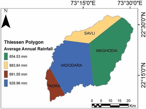
Based on past 56 years (1961 to 2016) rainfall data analysis of rain gauge stations across watershed, it was determined that the SPI indicates extremely dry years 1.8 % of the time, moderately dry years 10.7% of the time, moderately wet years 3.6% of the time, near normal years 73.2% of the time, very wet years 7.1% of the time and extremely wet years 3.6% of the time. Classification of annual rainfall of the study area based on SPI is shown in Table 5. The result therefore suggests that the overall drought events between these years were not severe. The precipitation analysis result suggests that the water shortage in the region is a management problem. This qualifies the area for identification of suitable sites for water storage. Also, computed annual rainfall for Vadodara, Savali, Padra and Waghodia rain gauge stations are 928.96, 891.56, 883.85 and 854.53 mm, respectively. The seasonal distribution of the precipitation in the study area varies and falls mostly as rain in monsoon season (June to September). Thiessen polygon of rain gauge stations is shown in Figure 4. Promoting rainwater harvesting in areas receiving less than 100 mm/year or more than 1000 mm/year of rains is not recommended (Kahinda et al. (2008); Mou, Wang, and Kung (1999); FAO (2003); Mati et al. (2006)). Water based activity are not feasible in areas that receive less than 100 mm/year of rain, also, there is no incentive to implement rain water harvesting schemes in areas with annual rains in excess of 1000 mm/year. Rainfall analysis of Vishamitri watershed shows potential to carry out water based activity in the area.

Figure 4. Thiessen polygon of rain gauge stations for Vishwamitri watershed.

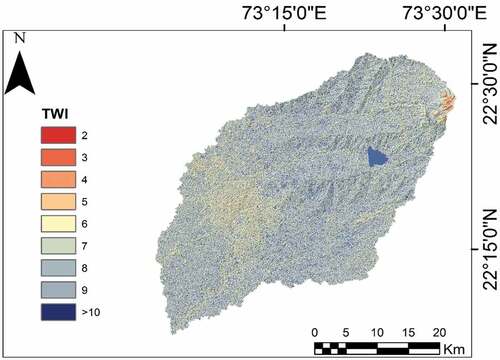
4.2. Topography wetness index (TWI)

High values of the TWI are found in converging and flat areas and are expected to have much water accumulation and low slope. In contrast, steep locations and diverging areas receive a small index value and have relatively lower water accumulation. Consequently, the index is a relative measure of the hydrological conditions of a given location in the landscape. Figure 5 shows the calculated TWI for the Vishwamitri watershed.

Figure 5. Spatial variation of topography wetness index across Vishwamitri watershed.

4.3. Generation of slope map using Topography Position Index (TPI)

Positive TPI values indicate that the target point location is higher than the average of its surroundings, as defined by the neighbourhood (ridges). Figure 7 shows conversion of elevation values to TPI along the cross section (shown in red colour in TPI map). Negative TPI values represent locations that are lower than their surroundings (valleys). TPI values near zero are either flat areas (where the slope is near zero) or areas of constant slope (where the slope of the point is significantly greater than zero). TPI for the study area is shown in Figure 6. Slope classification was done as suggested by Weiss (2001) and Jenness (2006). Slope plays a significant role in the amounts of runoff and sedimentation, the speed of water flow and the amount of material required to construct a dyke (the required height). Results shows (Table 6 and Figure 8) that maximum area belongs to flat class (35.45%), flat areas are never strictly horizontal, also, flat slopes lead to a decrease in the surface runoff velocity, which results in a longer period of time for the runoff to drain; there are gentle slopes in a seemingly flat area. Ponds are suitable for small flat areas with slopes 5%, 0.15% belongs to middle slope, nala bunds are suitable on moderate slopes of 5–10%, 12.49% area belongs to upper slope, terracing is suitable for steeper slopes of 5–30%. Ridges and upper slope together forms 30.79% of the area, they indicate least potential for rainwater harvesting because higher sloping land is inappropriate for constructing water storage structures. Valley and lower slope together constitutes for 33.58% of the area, small dams or check dams like structures are preferable on such sites.

Figure 6. Variation of topography position index across the Vishwamitri watershed.

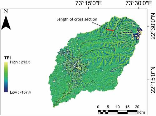
Figure 7. Comparison between the original DEM and TPI along the cross-sectional profile (red line).

Figure 8. Resulted slope map of the study area using TPI as basis of landform classification.

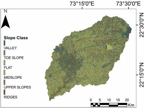
Table 5. Classification of annual rainfall based on SPI.

Classification	Years
Dry extreme years	2008
Moderately dry years	1972, 1974, 1986, 1987, 1999,2000
Moderately wet years	1983, 1994
Near normal years	1961, 1962, 1963, 1964, 1965, 1966, 1967, 1968, 1969, 1971, 1973, 1975, 1977, 1978, 1979, 1980, 1981, 1982, 1984, 1985, 1988, 1989, 1990, 1991, 1992, 1993, 1995, 1996, 1997, 1998, 2001, 2002, 2003, 2004, 2007, 2009, 2011, 2012, 2014, 2015, 2016
Very wet years	1976, 2006, 2010, 2013
Wet extreme years	1970, 2005

Table 6. Slope classifications using TPI as basis of landform classification for the study area.

Class	Description Breakpoints	Area (km^2)
Valley	TPI ≤ −4.6	255
Lower Slope	− 4.6< TPI ≤ −2.3	178
Flat Slope	−2.3 < TPI < 2.3, Slope ≤ 5°	457
Middle Slope	–2.3 < TPI < 2.3, Slope > 5°	2
Upper Slope	2.3 < TPI ≤ 4.6	161
Ridge	TPI > 4.6	236

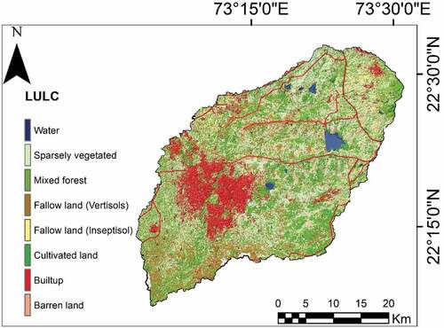
4.4. Land use/land cover

The land use/land cover map of the study area is shown in Figure 9, which reveals that there are seven major types of land use/land cover namely Waterbodies, Builtup, Mixed forest, Cultivated land, Barren land, Fallow land with vertisols dominance and Fallow land with inceptisols dominance. Major portion of the study area (about 35%) is Agricultural land (cultivated land, fallow land with vertisols dominance and fallow land with inseptisol dominance) followed by Sparsely vegetated (19%), Mixed forest (14%), Builtup (12%), Barren land (5%) and Water bodies (2%). Land-use classes such as barren land and sparsely vegetated land are generally recommended for water storage zones/structures. The results of accuracy assessment are given in Table 7.

Figure 9. Land use/land cover map of the Vishwamitri watershed.

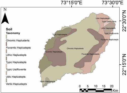
4.5. Soil texture

According to the classification based on soil texture, seven types of soils are found in the Vishwamitri watershed (Figure 10). Typic Ustifluvents and Fluventic Haplustepts correspond to HSG group A, Udic Haplustepts corresponds to HSG group B, Chromic Haplusterts and Typic Haplustepts correspond to HSG group C, and Lithic Haplustepts and Vertic Haplustepts corresponds to HSG group D. The most dominating soil, Chromic Haplusterts (HSG group C), covers 48.94% of the total watershed area. HSG-A has the lowest runoff potential (typically contains more than 90% sand and less than 10% clay), HSG-B has moderately low runoff potential (typically contains between 10 to 20% clay and 50 to 90% sand), HSG-C has moderately high runoff potential (typically contains between 20 to 40% clay and less than 50% sand) and HSG-D has high runoff potential (typically contains more than 40% clay and less than 50% sand) Ross et al. (2018).

Figure 10. Soil data based on soil texture collected from (NBSS & LUP).

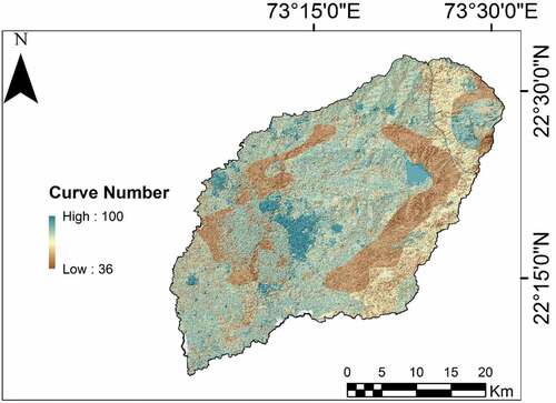
4.6. Curve Number (CN)

CN considers the relationship between land use/land cover and hydrologic soil group, which together make up the CN. The CN value varied from 36 to 100 for the study area (Figure 11) with mean value of 82.39 and standard deviation of 11.56, lower numbers indicate low runoff potential while larger numbers indicate an increased runoff potential. A CN value of 100 represents a condition of zero potential maximum retention that suggests an impermeable catchment having maximum runoff-generation capability. On the other hand, a CN value of 0 suggests an infinitely abstracting catchment having zero runoff-generation capability Jha et al. (2014). With this approach, the suitable locations for surface water storage zones/structures were located in areas with the highest capacity for runoff generation and nearby to existing drainage lines. Number of researchers applied the CN method to identify potential runoff-harvesting sites (e.g. De Winnaar, Jewitt, and Horan (2007); Jha et al. (2014); Krois and Schulte (2014)).

Figure 11. Variation of curve number across the Vishwamitri watershed.

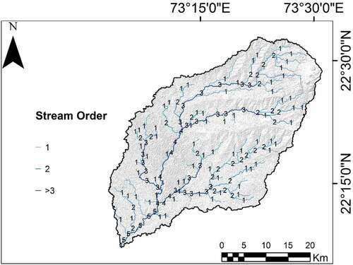
4.7. Stream order

Suitable zones/sites for surface water storage structures, all the1st, 2nd and 3rd order streams were extracted from the drainage network map and a stream-order buffer map was developed with a buffer distance of 50 m on both sides of the streams. It can be seen from the drainage network map (Figure 12) that the study area has a fifth order drainage network, with a good drainage network in the eastern portion. Length of the first order streams in the study area is nearly 294.5 km (about 52.9% of total length of drainage). The second and third order streams have also considerable drainage lengths, 124.7 km (22.4%) and 88.1 km (15.8%), respectively. The fourth order stream contributes to drainage with a length of 33.0 km, which accounts for 5.9% of the total drainage length. Mainly, the Vishwamitri River is a fifth order stream having a drainage length of 16.7 km (3.0%).

Figure 12. Drainage network map showing stream order of the Vishwamitri watershed.

4.8. Height above nearest drainage (HAND)

Low-lying land adjacent to streams is more susceptible to be flooded than higher land. HAND values for the study area varies from 0 to 749 m. HAND raster was prepared for the 4th and 5th order streams of Vishwamitri watershed as they are highly susceptible to flooding. On suitability scale, lower values were assigned for HAND values ranging from 0–2 metres as these areas are more prone to flooding, and it is not recommended to build water storage structure on such zones. Also, lower values were assigned on suitability scale for extremely high HAND values (greater than 48 metres) because higher HAND value means point moves away from the river. Figure 13 shows the Height above nearest drainage (HAND) map of the study area.

Figure 13. Height above nearest drainage (HAND) map of the Vishwamitri watershed.

4.9. Determining criteria weights using AHP

AHP provided a systematic approach to conduct MCDM. To derive suitability maps for potential runoff storage zones, the criteria maps have to be related to the result of the AHP. The AHP pair-wise matrix for the criteria used in this study is presented in Table 8. For all the five spatial layers the relative importance is derived. Thus, a common scale (0 % to 100%) is obtained from AHP procedure. As seen in Table 8, the most important criterion for decision-making is Slope (22.50%), followed by LULC (21.20%), CN (14.80%), HAND (14.50%), Stream order (14.40%) and TWI (12.60%). Calculated principal eigenvector is 6.47, which is computed with the square reciprocal matrix of pairwise comparisons between criteria. Since the AHP may have inconsistencies in establishing the values for the pairwise comparison matrix, it is important to calculate this level of inconsistency using the consistency ratio (CR). The CR of the pair-wise matrix is 7.5% (which is less than 10%) and thus the judgements made and compiled in the pair-wise matrix of Table 8 are acceptable. This implies that the comparisons were performed with good judgement, weightage for each criterion is suitable to weighted overlay.

Table 7. Accuracy assessment results.

LULC	Sub classes of LULC	Producer’s accuracy	User’s accuracy
Water	Water	1.00	1.00
Cultivated land	Cultivated land Crop 1	0.80	0.57
	Cultivated land Crop 2	0.60	0.67
	Sparsely vegetated	0.88	0.88
Barren land	Barren land	0.50	0.43
Fallow land (Vertisols dominance)	Fallow land 1 Vertisols dominance	0.60	0.86
	Fallow land 2 Vertisols dominance	1.00	0.60
Fallow land (Inseptisol dominance)	Fallow land 1 Inseptisol dominance	1.00	0.67
	Fallow land 2 Inseptisol dominance	0.75	1.00
Mixed forest	Mixed forest	0.33	0.25
Builtup	Builtup	1.00	0.86
	Mixed builtup 1	1.00	1.00
	Mixed builtup 2	0.56	1.00
	Kappa coefficient	0.74
	Overall Accuracy (%)	76.00

Table 8. Resulting weights for the criteria based on pairwise comparisons.

	Slope	TWI	LULC	Curve number	Stream order	HAND	Priority (%)	Rank
Slope	1	2	0.5	2	2	2	22.50	1
TWI	0.5	1	1	1	1	0.5	12.60	6
LULC	2	1	1	1	2	1	21.20	2
Curve number	0.5	1	1	1	0.5	2	14.80	3
Stream order	0.5	1	0.5	2	1	1	14.40	5
HAND	0.5	2	1	0.5	1	1	14.50	4

4.10. WOP within GIS

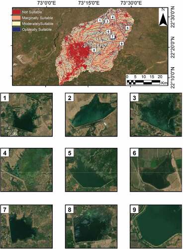
Potential runoff storage zones of the study area (Figure 14) was generated by integrating the thematic layers of slope, LULC, CN, HAND, stream order and TWI using WOP within GIS. Resulted raster was classified into four classes namely (a) Not suitable (b) Marginally Suitable (c) Moderately Suitable (d) Optimally Suitable. Result shows that 17% of the area is optimally suitable, 33.2% of the area is moderately suitable, 33.1% of the area is marginally suitable and 18.7% of the area is not suitable for water storage zones/structures. Sixteen suitable sites on such zones (optimally suitable class) have also been identified for water storage structures, as shown in Figure 15. Criteria of selection of these sites are: first, proximity of the sites to the agricultural fields. Second, sites should be on unused or barren land. Third, narrow cross-section of the valley with high shoulders to minimize the amount of construction material needed for building the small dams or check dams, nala bunds, gully plug and bundhis. Results are also confirmed by the already built water storage structures in derived potential runoff storage zones which are in optimally suitable class (Figure 16).

Figure 14. Potential runoff storage zones of the study area.

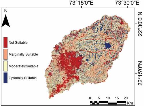
Figure 15. Identified sites for water storage structures on potential runoff storage zones.

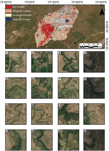
Figure 16. Already built water storage structures on the derived potential runoff storage zones.

5. Conclusion

The objective of this study was to identify potential runoff storage zones based on the various physical characteristics of the Vishwamitri watershed using a GIS-based conceptual framework that combines through AHP using MCDM method. Furthermore, the selection of factors (Slope, Land use/land cover, HAND, Stream order, CN, TWI) are based on review suggestions from several previous investigators. Results will help concerned authorities in the proficient arranging and execution of water-related plans and schemes, improve water shortage, reduce dependability on ground water and ensure sustainable water availability for local and agricultural purposes in the study area. It is recommended that the proposed suitability map be developed by the GIS technique for the study area may be implemented in the future to overcome growing water scarcity due to global/regional climate change. Since the approach and the analysis showed in this research have non-exclusive relevance, they are exceptionally valuable for other parts of the world, especially for developing countries, despite hydrological and agro-climatic variations. This approach is less time-consuming, more precise and can be utilized for identifying potential locations for different interventions for large watersheds.

Disclosure Statement

On behalf of all authors, the corresponding author states that there is no conflict of interest.

References

- Adegoke, C. W., and A. O. Sojobi. 2015. “Climate Change Impact on Infrastructure in Osogbo Metropolis, South-west Nigeria.” Journal of Emerging Trends in Engineering and Applied Sciences 6: 156–165.
- Ågren, A. M., W. Lidberg, M. Strömgren, J. Ogilvie, and P. A. Arp. 2014. “Evaluating Digital Terrain Indices for Soil Wetness Mapping–a Swedish Case Study.” Hydrology and Earth System Sciences 18 (9): 3623–3634. doi:10.5194/hess-18-3623-2014.
- Akinsanola, A. A., and K. O. Ogunjobi. 2014. “Analysis of Rainfall and Temperature Variability over Nigeria. Global Journal of Human Social Sciences.” Geography & Environmental GeoSciences 14 (3): 1–18.
- Al-Adamat, R. 2008. “GIS as a Decision Support System for Siting Water Harvesting Ponds in the Basalt Aquifer/NE Jordan.” Journal of Environmental Assessment Policy and Management 10 (2): 189–206. doi:10.1142/S1464333208003020.
- Ammar, A., M. Riksen, M. Ouessar, and C. Ritsema. 2016. “Identification of Suitable Sites for Rainwater Harvesting Structures in Arid and Semi-arid Regions: A Review.” International Soil and Water Conservation Research 4 (2): 108–120. doi:10.1016/j.iswcr.2016.03.001.
- Berking, J., B. Beckers, and B. Schütt. 2010. “Runoff in Two Semi-Arid Watersheds in a Geoarcheological Context: A Case Study of Naga, Sudan, and Resafa, Syria.” Geoarchaeology 25: 815–836. doi:10.1002/gea.v25:6.
- Beven, K. J., and M. J. Kirkby. 1979. “A Physically Based, Variable Contributing Area Model of Basin Hydrology.” Hydrological Sciences Bulletin 24 (1): 43–69. doi:10.1080/02626667909491834.
- Bitterman, P., E. Tate, K. J. Van Meter, and N. B. Basu. 2016. “Water Security and Rainwater Harvesting: a Conceptual Framework and Candidate Indicators.” Applied Geography 76: 75-84. doi:10.1016/j.apgeog.2016.09.013.
- Bjelanovic, I. 2016. “Predicting Forest Productivity Using Wet Areas Mapping and Other Remote Sensed Environmental Data.”
- Burnside, N., R. Smith, and S. Waite. 2002. “Habitat Suitability Modelling for Calcareous Grassland Restoration on the South Downs, United Kingdom.” Journal of Environmental Management 65 (2): 209e221. doi:10.1006/jema.2002.0546.
- Burrough, P. A., P. F. van Gaans, and R. A. MacMillan. 2000. “High-resolution Landform Classification Using Fuzzy K-means.” Fuzzy Sets and Systems 113 (1): 37–52. doi:10.1016/S0165-0114(99)00011-1.
- De Winnaar, G., G. P. W. Jewitt, and M. Horan. 2007. “A GIS-based Approach for Identifying Potential Runoff Harvesting Sites in the Thukela River Basin, South Africa.” Physics and Chemistry of the Earth 32: 1058–1067. doi:10.1016/j.pce.2007.07.009.
- Deng, Y. 2007. “New Trends in Digital Terrain Analysis: Landform Definition, Representation, and Classification.” Progress in Physical Geography 31 (4): 405–419. doi:10.1177/0309133307081291.
- Deumlich, D., R. Schmidt, and M. Sommer. 2010. “A Multiscale Soil–landform Relationship in the Glacial-drift Area Based on Digital Terrain Analysis and Soil Attributes.” Journal of Plant Nutrition and Soil Science 173: 843–851. doi:10.1002/jpln.v173.6.
- Dilts, T. E. 2015. “Topography Tools for ArcGIS 10.1.” http://www.arcgis.com/home/item.html?id=b13b3b40fa3c43d4a23a1a09c5fe96b9
- Durga Rao, K. H. V., and M. K. Bhaumik. 2003. “Spatial Expert Support System in Selecting Suitable Sites for Water Harvesting Structures—A Case Study of Song Watershed, Uttaranchal, India.” Geocarto International 18 (4): 43–50. doi:10.1080/10106040308542288.
- FAO. 2003. “Land and Water Digital Media Series, 26. Training Course on RWH (CDROM). Planning of Water Harvesting Schemes, Unit 22.” Food and Agriculture Organization of the United Nations. Rome: FAO.
- Feldman, A. D. 2000. “Hydrologic Modeling System HEC-HMS: Technical Reference Manual.” US Army Corps of Engineers, Hydrologic Engineering Center.
- Francés, A. P., and M. W. Lubczynski. 2011. “Topsoil Thickness Prediction at the Catchment Scale by Integration of Invasive Sampling, Surface Geophysics, Remote Sensing and Statistical Modeling.” Journal of Hydrology 405: 31–47. doi:10.1016/j.jhydrol.2011.05.006.
- Gallant, J. C., and J. P. Wilson. 2000. “Primary Topographic Attributes.” In Terrain Analysis: Principles and Applications, edited by J. P. Wilson and J. C. Gallant, 51–85. New York: Wiley.
- Ghani, M. W., M. Arshad, A. Shabbir, N. Mehmood, and I. Ahmad. 2013. “Investigation of Potential Water Harvesting Sites at Potohar Using Modeling Approach.” Pakistan Journal of Agricultural Sciences 50 (4): 723-729.
- Hamdani, N., and A. Baali. 2019. “Height above Nearest Drainage (HAND) Model Coupled with Lineament Mapping for Delineating Groundwater Potential Areas (GPA).” Groundwater for Sustainable Development 9: 100256. doi:10.1016/j.gsd.2019.100256.
- Hengl, T., and H. I. Reuter, Eds.. 2008. Geomorphometry: Concepts, Software, Applications. Vol. 33. Newnes. Amsterdam, The Netherlands: Elsevier.
- Hojati, M., and M. Mokarram. 2016. “Determination of a Topographic Wetness Index Using High Resolution Digital Elevation Models.” European Journal of Geography 7: 41–52.
- Illés, G., G. Kovács, and B. Heil. 2011. “Comparing and Evaluating Digital Soil Mapping Methods in a Hungarian Forest Reserve.” Canadian Journal of Soil Science 91: 615–626. doi:10.4141/cjss2010-007.
- IMSD. 1995. “Integrated Mission for Sustainable Development Technical Guidelines.” National Remote Sensing Agency, Department of Space, Govt. of India.
- Iwahashi, J., and R. J. Pike. 2007. “Automated Classifications of Topography from DEMs by an Unsupervised Nested-means Algorithm and a Three-part Geometric Signature.” Geomorphology 86 (3–4): 409–440. doi:10.1016/j.geomorph.2006.09.012.
- Jenness, J. 2006. “Topographic Position Index (Tpi_jen.avx) Extension for ArcView 3.x, V.1.3a.” http://www.jennessent.com/arcview/tpi.htm
- Jenson, Susan K., and Julia O. Domingue. 1988. “Extracting Topographic Structure from Digital Elevation Data for Geographic Information System Analysis.” Photogrammetric Engineering and Remote Sensing 54 (11): 1593-1600.
- Jha, M. K., V. M. Chowdary, Y. Kulkarni, and B. C. Mal. 2014. “Rainwater Harvesting Planning Using Geospatial Techniques and Multicriteria Decision Analysis.” Resources, Conservation and Recycling 83: 96–111. doi:10.1016/j.resconrec.2013.12.003.
- Kahinda, J. M., E. S. B. Lillie, A. E. Taigbenu, M. Taute, and R. J. Boroto. 2008. “Developing Suitability Maps for Rainwater Harvesting in South Africa.” Physics and Chemistry of the Earth, Parts A/B/C 33 (8–13): 788–799. doi:10.1016/j.pce.2008.06.047.
- Karimi, H., and H. Zeinivand. 2019. “Integrating Runoff Map of a Spatially Distributed Model and Thematic Layers for Identifying Potential Rainwater Harvesting Suitability Sites Using GIS Techniques.” Geocarto International 1–20. doi:10.1080/10106049.2019.1608590.
- Krois, J., and A. Schulte. 2014. “GIS-based Multi-criteria Evaluation to Identify Potential Sites for Soil and Water Conservation Techniques in the Ronquillo Watershed, Northern Peru.” Applied Geography 51: 131–142. doi:10.1016/j.apgeog.2014.04.006.
- Kumar, T., and D. C. Jhariya. 2017. “Identification of Rainwater Harvesting Sites Using SCS-CN Methodology, Remote Sensing and Geographical Information System Techniques.” Geocarto International 32 (12): 1367–1388. doi:10.1080/10106049.2016.1213772.
- Lesschen, J. P., K. Kok, P. H. Verburg, and L. H. Cammeraat. 2007. “Identification of Vulnerable Areas for Gully Erosion under Different Scenarios of Land Abandonment in Southeast Spain.” Catena 71: 110–121. doi:10.1016/j.catena.2006.05.014.
- Liu, H., R. Bu, J. Liu, W. Leng, Y. Hu, L. Yang, and H. Liu. 2011. “Predicting the Wetland Distributions under Climate Warming in the Great Xing’an Mountains, Northeastern China.” Ecological Research 26: 605–613. doi:10.1007/s11284-011-0819-2.
- Liu, M., Y. Hu, Y. Chang, X. He, and W. Zhang. 2009. “Land Use and Land Cover Change Analysis and Prediction in the Upper Reaches of the Minjiang River, China.” Environmental Management 43: 899–907. doi:10.1007/s00267-008-9263-7.
- Loritz, R., A. Kleidon, C. Jackisch, M. Westhoff, U. Ehret, H. Gupta, and E. Zehe. 2019. “A Topographic Index Explaining Hydrological Similarity by Accounting for the Joint Controls of Runoff Formation.” Hydrology and Earth System Sciences 23 (9): 3807–3821. doi:10.5194/hess-23-3807-2019.
- Mahmoud, S. H., and A. A. Alazba. 2014. “The Potential of in Situ Rainwater Harvesting in Arid Regions: Developing a Methodology to Identify Suitable Areas Using GISbased Decision Support System.” Arabian Journal of Geosciences 8: 1–13.
- Malczewski, J. 1999. GIS and Multicriteria Decision Analysis, 392. New York: John Wiley & Sons, Inc.
- Mati, B., T. De Bock, M. Malesu, E. Khaka, A. Oduor, M. Meshack, and V. Oduor. 2006. “Mapping the Potential of Rainwater Harvesting Technologies in Africa. A GIS Overview on Development Domains for the Continent and Ten Selected Countries.” Technical Manual No. 6. World Agroforestry Centre (ICRAF), 126. Nairobi, Kenya: Netherlands Ministry of Foreign Affairs.
- McGarigal, K., S. Tagil, and S. Cushman. 2009. “Surface Metrics: An Alternative to Patch Metrics for the Quantification of Landscape Structure.” Landscape Ecology 24: 433–450. doi:10.1007/s10980-009-9327-y.
- McKee, T. B., N. J. Doesken, and J. Kleist. 1993 January 17–22. “The Relationship of Drought Frequency and Duration to Time Scale.” In Proceedings of the Eighth Conference on Applied Climatology, 179–184. Anaheim, California. Boston: American Meteorological Society.
- Mora-Vallejo, A., L. Claessens, J. Stoorvogel, and G. B. M. Heuvelink. 2008. “Small Scale Digital Soil Mapping in Southeastern Kenya.” Catena 76: 44–53. doi:10.1016/j.catena.2008.09.008.
- Mou, H., H. Wang, and H. Kung. 1999. “Division Study of Rainwater Utilization in China.” In 9th International Rainwater Catchment System Conference, Brazil.
- Nobre, A. D., L. A. Cuartas, M. Hodnett, C. D. Rennó, G. Rodrigues, A. Silveira, M. Waterloo, and S. Saleska. 2011. “Height above the Nearest Drainage–a Hydrologically Relevant New Terrain Model.” Journal of Hydrology 404 (1–2): 13–29. doi:10.1016/j.jhydrol.2011.03.051.
- Patterson, J. J. 2008. “Late Holocene Land Use in the Nutzotin Mountains: Lithic Scatters, Viewsheds, and Resource Distribution.” Arctic Anthropology 45: 114–127. doi:10.1353/arc.0.0009.
- Pauw, E. D., T. Oweis, and J. Youssef. 2008. Integrating Expert Knowledge in GIS to Locate Biophysical Potential for Water Harvesting: Methodology and a Case Study for Syria, 59. Aleppo, Syria: ICARDA.
- Pracilio, G., K. Smettem, D. Bennett, R. Harper, and M. Adams. 2006. “Site Assessment of a Woody Crop Where a Shallow Hardpan Soil Layer Constrained Plant Growth.” Plant and Soil 288: 113–125. doi:10.1007/s11104-006-9098-z.
- Prasad, H. C., P. Bhalla, and S. Palria. 2014. “Site Suitability Analysis of Water Harvesting Structures Using Remote Sensing and GIS-A Case Study of Pisangan Watershed, Ajmer District, Rajasthan.” The International Archives of Photogrammetry, Remote Sensing and Spatial Information Sciences 40 (8): 1471. doi:10.5194/isprsarchives-XL-8-1471-2014.
- Quinn, P., K. Beven, P. Chevallier, and O. Planchon. 1991. “The Prediction of Hillslope Flow Paths for Distributed Hydrological Modelling Using Digital Terrain Models.” Hydrological Processes 5: 59–79. doi:10.1002/()1099-1085.
- Rana, V. K., and T. M. V. Suryanarayana. 2019a. “Visual and Statistical Comparison of ASTER, SRTM, and Cartosat Digital Elevation Models for Watershed.” Journal of Geovisualization and Spatial Analysis 3 (2): 12. doi:10.1007/s41651-019-0036-z.
- Rana, V. K., and T. M. V. Suryanarayana. 2019b. “Evaluation of SAR Speckle Filter Technique for Inundation Mapping.” Remote Sensing Applications: Society and Environment 16: 100271. doi:10.1016/j.rsase.2019.100271.
- Rennó, C. D., A. D. Nobre, L. A. Cuartas, J. V. Soares, M. G. Hodnett, J. Tomasella, and M. J. Waterloo. 2008. “HAND, a New Terrain Descriptor Using SRTM-DEM: Mapping Terra-firme Rainforest Environments in Amazonia.” Remote Sensing of Environment 112 (9): 3469–3481.
- Rizeei, H. M., B. Pradhan, and M. A. Saharkhiz. 2018. “Surface Runoff Prediction regarding LULC and Climate Dynamics Using Coupled LTM, Optimized ARIMA, and GIS-based SCS-CN Models in Tropical Region.” Arabian Journal of Geosciences 11 (3): 53. doi:10.1007/s12517-018-3397-6.
- Ross, C. W., L. Prihodko, J. Anchang, S. Kumar, W. Ji, and N. P. Hanan. 2018. “HYSOGs250m, Global Gridded Hydrologic Soil Groups for Curve-number-based Runoff Modeling.” Scientific Data 5: 180091. doi:10.1038/sdata.2018.91.
- Rozos, D., G. D. Bathrellos, and H. D. Skillodimou. 2011. “Comparison of the Implementation of Rock Engineering System and Analytic Hierarchy Process Methods, upon Landslide Susceptibility Mapping, Using GIS: A Case Study from the Eastern Achaia County of Peloponnesus, Greece.” Environmental Earth Sciences 63 (1): 49–63. doi:10.1007/s12665-010-0687-z.
- Saaty, T. L. 1977. “A Scaling Method for Priorities in Hierarchical Structures.” Journal of Mathematical Psychology 15 (3): 234–281. doi:10.1016/0022-2496(77)90033-5.
- Saaty, T. L. 1987. “Rank Generation, Preservation, and Reversal in the Analytic Hierarchy Decision Process.” Decision Sciences 18 (2): 157e177. doi:10.1111/deci.1987.18.issue-2.
- Saaty, T. L. 1990. “How to Make a Decision: The Analytic Hierarchy Process.” European Journal of Operational Research 48 (1): 9e26. doi:10.1016/0377-2217(90)90057-I.
- Singh, L. K., M. K. Jha, and V. M. Chowdary. 2017. “Multi-criteria Analysis and GIS Modeling for Identifying Prospective Water Harvesting and Artificial Recharge Sites for Sustainable Water Supply.” Journal of Cleaner Production 142: 1436–1456. doi:10.1016/j.jclepro.2016.11.163.
- Sørensen, R., and J. Seibert. 2007. “Effects of DEM Resolution on the Calculation of Topographical Indices: TWI and Its Components.” Journal of Hydrology 347 (1–2): 79–89. doi:10.1016/j.jhydrol.2007.09.001.
- Strahler, A. N. 1957. “Quantitative Analysis of Watershed Geomorphology.” Eos, Transactions American Geophysical Union 38 (6): 913–920. doi:10.1029/TR038i006p00913.
- Tagil, S., and J. Jenness. 2008. “GIS-based Automated Landform Classification and Topographic, Landcover and Geologic Attributes of Landforms around the Yazoren Polje, Turkey.” Journal Of Applied Sciences 8: 910–921. doi:10.3923/jas.2008.910.921.
- Tripathi, S. S. 2018. “Impact of Land Use Land Cover Change on Runoff Using RS & GIS and Curve Number.” International Journal of Basic and Applied Agricultural Research 16 (3): 224–227.
- Weerasinghe, H., U. A. Schneider, and A. Loew. 2011. “Water Harvest-and Storage-location Assessment Model Using GIS and Remote Sensing.” Hydrology and Earth System Sciences Discussions 8 (2): 3353–3381. doi:10.5194/hessd-8-3353-2011.
- Weiss, A. D. 2001. “Topographic Position and Landforms Analysis.” Poster Presentation, ESRI Users Conference, San Diego, CA.
- Wilson, J. P., and J. C. Gallant. 2000. “Digital Terrain Analysis.” Terrain Analysis: Principles and Applications 6 (12): 1–27.
- Wu, R. S., G. L. L. Molina, and F. Hussain. 2018. “Optimal Sites Identification for Rainwater Harvesting in Northeastern Guatemala by Analytical Hierarchy Process.” Water Resources Management 32 (12): 4139–4153. doi:10.1007/s11269-018-2050-1.