BIM/GIS integration for web GIS-based bridge management

ABSTRACT

Integration of Building Information Modelling (BIM) and Geographic Information System (GIS) can benefit both the Architecture, Engineering and Construction/Facility Management (AEC/FM) domain, and the geospatial industry. For GIS, BIM is a promising source of three-dimensional (3D) building information that can be used in the study of smart city, green building, big data, etc. The underlying data transformation from Industry Foundation Classes (IFC) to shapefile enables GIS to use the rich building information. However, this transformation is difficult due to the different modelling methods used by IFC and shapefile. IFC generally represents 3D objects using boundary representation (Brep), swept solid, constructive solid geometry (CSG), clipping and mapped representation, while shapefile only uses Brep. In addition, the use of different coordinate systems also contributes to the geometry transformation issue. Among all the solid modelling methods used by IFC, Brep and swept solid are the most often used two methods. Compared with Brep, the transformation of swept solid is more challenging as each type of profile for swept solid defined in IFC has to be properly interpreted and converted. This paper develops algorithms to interpret the commonly used profiles of swept solid for the transformation of IFC into shapefile. A bridge model is used to validate the proposed method, and a Web GIS-based bridge management system is developed to demonstrate a possible usage of the transformed shapefile model.

KEYWORDS:

• Building information modelling
• geographic information system
• 3d
• geometry transformation
• smart city
• industry foundation classes
• shapefile

1. Introduction

BIM refers to Building Information Model or Building Information Modelling. The former refers to virtual 3D building models with rich building information and the latter means the process of producing and processing these models (Eastman et al. 2011; Li et al. 2017). BIM has been widely used in the Architecture, Engineering and Construction/Facility Management (AEC/FM) domain (Zhu et al. 2018; Tan et al. 2018; Li et al. 2019), covering the entire lifecycle of a construction project, including plan, design, construction, operation, and dismantling (Volk, Stengel, and Schultmann 2014; Azhar 2011).

BIM can benefit GIS by providing detailed 3D building models. GIS was initially focused on 2D dataset, and its capability in 3D data creation and processing is quite limited (Zhu et al. 2018). By integrating BIM into GIS, the spatial analysis can be conducted at a finer scale. For example, indoor networks can be built from building models for emergency response (Teo and Cho 2016). The influence of noise can be assessed at room scale rather than at regional scale (Deng, Cheng, and Anumba 2016a), and the influence of flood can be evaluated at building scale (Amirebrahimi et al. 2016b), which enables more accurate flood damage assessment. For AEC/FM domain, compared with BIM-only approach, approaches through BIM/GIS integration can be more promising in two ways: (1) spatial analysis can be introduced for better problem solving, considering BIM barely has analysis functionality, and (2) built structures can be connected with their surroundings by introducing environmental data, such as road network and terrain data.

The underlying data exchange is essential to the success of industry-level BIM/GIS integration. In the AEC/FM domain, Industry Foundation Classes (IFC) is the most commonly used data schema for building information exchange among different vendors (Amirebrahimi et al. 2016a), while shapefile is widely used in the geospatial industry (Zhu et al. 2018; Xu et al. 2016; Tashakkori, Rajabifard, and Kalantari 2015). Therefore, it is reasonable to believe that realizing the transformation of IFC into shapefile would greatly benefit GIS in 3D modelling and other studies in GIS based on 3D building models, such as smart city and green building (Zhu et al. 2019b).

Generally, in the field of modelling, there are three basic methods for solid modelling, including boundary representation (Brep), constructive solid geometry (CSG) and sweeping. IFC also uses these terms and has defined IfcSolidModel, which is the common abstract supertype of Brep, CSG representation, sweeping representation and other suitable solid representation schemes. In addition, IFC takes one step further and has defined many sub-types of these methods, such as advanced swept solid. Among them, Brep and swept solid are the most common methods.

The transformation of swept solid is more difficult than Brep. The transformation of Brep (IFC) to Brep (shapefile) is a matter of coordinate system transformation (CST) and standard alignment, as IFC and shapefile use different coordinate systems and have different definitions for a closed ring (a face), which is the most basic unit of Brep (ESRI 2018). In contrast, in terms of the transformation of swept solid, besides the CST problem, additional algorithms are needed to regenerate Brep from sweep parameters, i.e., swept area (also known as profile in IFC), extrusion direction and depth.

The transformation of swept solid generally has two steps: The first is to transform the swept area into a closed ring (initial ring), which is a sequence of points; the second step is to build Brep faces meeting the requirement of multipatch (a shapefile type for 3D geometry) standard using the initial ring, extrusion direction and depth. These two steps are critical to geometry transformation, especially the first step. Transforming swept area into the initial ring is challenging because of the large number of profiles defined by IFC. IFC has defined various sweeping profiles, including 12 parameterized profiles, 2 arbitrary profiles and another 2 approaches that support more complicated profiles (buildingSMART 2019).

Parameterized profiles, in IFC, are defined by certain parameters (Azhar, Khalfan, and Maqsood 2015). For example, the circle profile is defined by its centre and radius, and the rectangle profile is defined by its length and width. During geometry transformation, closed rings are to be generated from these parameters to approximate the swept areas.

In this study, the most often used profiles, such as circle profile, rectangle profile, I-shape profile and arbitrary closed profile will be studied, and algorithms for converting these profiles into closed initial rings will be developed for the ultimate geometry transformation of IFC into shapefile. Lastly, a bridge management system will be developed based on Web GIS to show a possible usage of the transformed shapefile bridge model.

The remainder of the paper is organized as follows: Section 2 introduces key aspects of BIM/GIS integration regarding data formats and transformation. Section 3 presents the proposed method for IFC transformation. Section 4 conducts the experiment and shows the result. Discussion is presented in Section 5, and Section 6 concludes the paper.

2. Formats and transformation in BIM/GIS integration

IFC is the representative data schema from the BIM side for BIM/GIS integration. It is a growing standard providing a semantic data model for building information. According to buildingSMART (buildingSMART 2019a), the latest IFC standard is IFC 4.1, which has totally defined 21 building elements, such as beam ($IfcBeam$), member ($IfcMember$), slab ($IfcSlab$), plate ($IfcPlate$), column ($IfcColumn$), covering ($IfcCovering$), and building element proxy ($IfcBuildingElementProxy$).

On the GIS side, primarily, two data formats or standards are being used, i.e., City Geography Markup Language (CityGML) (Deng, Cheng, and Anumba 2016b) and shapefile (Isikdag, Zlatanova, and Underwood 2013; Zhu et al. 2019a). Compared with CityGML, shapefile is more flexible in receiving BIM information. CityGML is an XML-based open data model for the storage and exchange of virtual 3D city models. When CityGML is used, more challenges have to be solved, such as mapping of classes, mapping of level of detail (LoD) between IFC and CityGML and restrict geometry transformation from solid models to surface models. In addition, in terms of modelling method, CityGML mainly uses surface models, while shapefile uses solid models which are more advanced than surface models. This means shapefile has greater potential than CityGML, for example, in 3D printing, and the geometry transformation between BIM and GIS can be achieved in an easier manner. There are other formats being used in BIM/GIS integration, such as Geography Markup Language (GML) (Amirebrahimi et al. 2016a) and Geodatabase (Teo and Cho 2016; Isikdag 2006), but they are not as often used as CityGML and shapefile.

There are not too many tools available for the transformation of IFC to shapefile. According to literature, Feature Manipulation Engine (FME) and Data Interoperability for ArcGIS (DIA) are the most frequently used commercial tools. However, they are not reliable enough as they may crash during operation (Zhu, Wang, and Wang 2018; Boyes, Ellul, and Irwin 2017). Another potential tool is Open CASCADE. Open CASCADE is an open-source software development kit (SDK) mainly used in areas such as computer-aided design (CAD), computer-aided manufacturing (CAM) and computer-aided engineering (CAE) for processing and visualizing 3D objects (SAS 2019b). However, converting IFC to shapefile using Open CASCADE is still problematic and not practical by far. This is mainly due to the complexity of the Brep format used by Open CASCADE (SAS 2019a) and the considerable workload needed to bridge the geometry gap between Breps used by Open CASCADE and shapefile. In contrast, the study presented in this paper provides an easier and practical approach to transform BIM models that can be saved for further use in GIS.

3. Methodology

3.1. Data

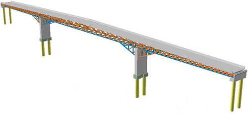
A steel-concrete composite bridge (Figure 1), with a width of 8.5 metres and a length of 223 metres, is used in this study to validate the proposed method. Bridges, built structures for the purpose of providing passage over obstacles such as body of water, valley or road, are very important infrastructure, especially in major cities, for providing safe and efficient transportation along with roads. The virtual bridge model was built using Tekla for a project in design stage and then exported as an IFC file. This model contains 608 entities belonging to 5 types of components, including beam, column, footing, member and slab. The types of entity and their quantity are presented in Table 1.

Figure 1. Bridge model used in this study

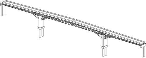
Table 1. Building element types and quantity

Entity	IFC class	Quantity
Beam	IfcBeam	195
Column	IfcColumn	11
Footing	IfcFooting	6
Member	IfcMember	380
Slab	IfcSlab	16

All these entities were modelled using swept solid but with different profiles. A script was written to check the profile used by each entity. Profiles used by each IFC class are presented in Table 2.

Table 2. Profiles used by entities

	Arbitrary	Circle	I-shape	Rectangle	Total
Beam	0	0	195	0	195
Column	0	8	3	0	11
Footing	0	0	0	6	6
Member	0	0	380	0	380
Slab	16	0	0	0	16
Total	16	8	578	6	608

3.2. Geometry transformation

3.2.1. Initial ring acquirement

The initial ring is generated from the parameters of swept area/profile. In the bridge model, four types of profile are being used, i.e., arbitrary profile, circle profile, I-shape profile and rectangle profile. Examples of arbitrary profile, rectangle profile and circle profile are presented in Figure 2 (Zhu et al. 2019b).

Figure 2. Example of (a) arbitrary profile, (b) rectangle profile and (c) circle profile

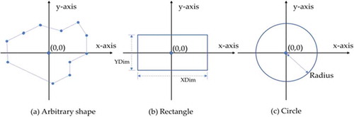
Since the arbitrary profile contains a set of points that form a closed ring, the initial ring can be obtained by extracting all the points in an arbitrary profile. The circle profile is defined by the circle centre and its radius. The initial ring can be obtained by the equation as follows:

(1) $\left\{\begin{array}{c}X=R\times cos\theta +x\\ Y=R\times sin\theta +y\end{array}\left(0\le \theta \le 2\pi \right)\right.$(1)

where $X$ and $Y$ are coordinates of points in the ring, $R$ is the radius of the circle, $x$ and $y$ are coordinates of the circle centre.

The rectangle profile is defined by its length ($L$) and width ($W$). The initial ring from rectangle profile can be represented as follows:

(2) $\begin{array}{rl}& \left[\left[L/2,W/2\left],\right[L/2,-W/2\left],\right[-L/2,-W/2\right],\right.\\ & \left.\left[-L/2,W/2\left],\right[L/2,W/2\right]\right]\end{array}$(2)

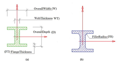
Compared with arbitrary profile, circle profile and rectangle profile, the conversion of the I-shape profile requires more steps. I-shape profile is defined by five parameters, including overall width ($W$), overall depth ($D$), web thickness ($WT$), flange thickness ($FT$) and fillet radius ($FR$) in its own 2D local coordinate system. Depending on whether fillet radius is given, I-shape profile has two subtypes, I-shape without fillet radius (Figure 3(a)) and I-shape with fillet radius (Figure 3(b)) (buildingSMART 2019b). From these parameters, the coordinates of points forming the initial ring can be obtained.

Figure 3. I-shape profiles (a) without fillet radius and (b) with fillet radius

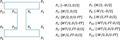
The initial ring (Figure 4) derived from I-shape without fillet radius can be represented as:

(3) $\left[P_1,P_2,P_3,P_4,P_5,P_6,P_7,P_8,P_9,P_{10},P_{11},P_{12},P_1\right]$(3)

Figure 4. Initial ring from I-shape without fillet radius

The initial ring (Figure 5) from I-shape with fillet radius is similar to the one from I-shape without fillet radius. However, $P_4$, $P_5$,$P_{10}$ and$P_4$ are replaced by $r_1$,$r_2$,$r_3$ and $r_4$ respectively.

Figure 5. Initial ring from I-shape with fillet radius

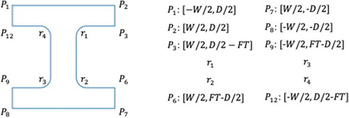
$r_1$,$r_2$,$r_3$ and $r_4$ each contains a sequence of points forming a quarter circle. They can be obtained through the following equation:

(4) $r_1:\left\{\begin{array}{c}X=FR\times cos\theta +\frac{WT}{2}+FR\\ Y=FR\times sin\theta +\frac{D}{2}-FT-FR\end{array}\left(\pi /2\le \theta \le \pi \right)\right.$(4)

(5) $r_2:\left\{\begin{array}{c}X=FR\times cos\theta +\frac{WT}{2}+FR\\ Y=FR\times sin\theta +FT+FR-\frac{D}{2}\end{array}\left(\pi \le \theta \le 1.5\pi \right)\right.$(5)

(6) $r_3:\left\{\begin{array}{c}X=FR\times cos\theta -\frac{WT}{2}-FR\\ Y=FR\times sin\theta +FT+FR-\frac{D}{2}\end{array}(1.5\pi \le \theta \le 2\pi \right.)$(6)

(7) $r_4:\left\{\begin{array}{c}X=FR\times cos\theta -\frac{WT}{2}-FR\\ Y=FR\times sin\theta +\frac{D}{2}-FT-FR\end{array}\left(0\le \theta \le \pi /2\right)\right.$(7)

where $X$ and $Y$ are coordinates of points in $r_1$,$r_2$,$r_3$ and $r_4$.

Therefore, the initial ring derived from I-shape with fillet radius can be represented as:

(8) $\left[P_1,P_2,P_3,r_1,r_2,P_6,P_7,P_8,P_9,r_3,r_4,P_{12},P_1\right]$(8)

3.2.2. Brep generation

After obtaining the initial ring, extrusion direction and depth, Brep can then be generated by two steps:

The first step is coordinate system transformation. BIM and GIS, or IFC and shapefile, use coordinate systems in a different way. IFC uses local coordinate systems (LCS), and each element has its own LCS. For example, a building has its own coordinate system, a story in the building also has its own coordinate system. These coordinate systems are, however, not independent. They together form a local coordinate system chain from the element-level LCS to the site-level LCS (Zhu et al. 2019b). In contrast, shapefile usually uses geographic coordinate system (GCS), such as WGS1984, and each element is defined in the same coordinate system.

The coordinate system transformation can be completed using the equation as follows (Zhu et al. 2019b):

(9) $\left[x\prime y\prime z\prime \right]=\left[\begin{array}{ccc}\mathrm{x}& \mathrm{y}& \mathrm{z}\end{array}\right]\times {\left({{\left[\begin{array}{ccc}\vec{\mathrm{x}}& \vec{\mathrm{y}}& \vec{\mathrm{z}}\end{array}\right]}^{\mathrm{T}}}^{-1}\right)}^{\mathbf{T}}+\left[x_0{y}_0{z}_0\right]$(9)

where $x\prime$, $y\prime$, and $z\prime$ are the transformed coordinates; $x$, $y$, and $z$ are the initial coordinates; $x_0$, $y_0$, and $z_0$ are the origin shift, $\overrightarrow{x}$,$\overrightarrow{y}$ and $\overrightarrow{z}$ are $3\times 1$ vectors indicating the direction of the initial x-axis, y-axis and z-axis, respectively.

The second step is to build Brep using the extracted parameters, as shown in Figure 6.

Figure 6. Generating Brep using extrusion parameters, i.e., initial ring and extrusion path

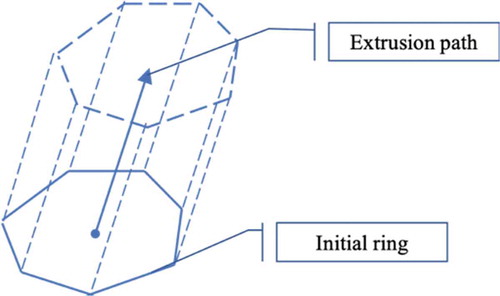
The extrusion path can be obtained by:

(10) $Extrusionpath=extrusiondirection\times depth$(10)

The detailed process has been presented by another relevant paper (Zhu et al. 2019b). In situations where building models are not defined in GCS, a 3D geo-referencing process is needed (Zhu et al. 2017).

The transformation is completed by several Python packages, such as IfcOpenShell for parsing IFC file, Pyshp for shapefile reading and writing, and Numpy for numbers and matrix processing.

3.3. Development of bridge management system

In this study, a bridge management system is to be developed using Web GIS technology to demonstrate a potential usage of the transformed shapefile model. This system will use the transformed bridge model to realize functions, such as model visualization, model attributes query, and real-time structural health monitoring.

Hypertext Markup Language (HTML), Cascading Style Sheets (CSS) and JavaScript are basic tools for the development of any web-based application. In this study, more advanced tools such as Dojo, jQuery, Rickshaw and Bootstrap will be used. In addition, ArcGIS API for JavaScript is used to access and manipulate the transformed bridge model. The relationship between Dojo, jQuery, Rickshaw, Bootstrap and JavaScript, HTML, CSS is presented in Figure 7.

Figure 7. Tools used in the development of the system

4. Results

4.1. Transformed model

Each transformed bridge component is shown in Table 3. The shapefile model is visualized using ArcScene, and the IFC model is visualized using FZK Viewer. In terms of appearance, there is no difference between IFC models and shapefile models.

Table 3. Side-by-side comparison of IFC model and shapefile model

	IFC	Shapefile
Beam
Column
Footing
Member
Slab

By assembling all the components, the final transformed bridge model can be obtained, which is represented in Figure 8.

Figure 8. The transformed bridge model visualized using ArcScene

The quantity of each element type is calculated to assess the transformation quality, which is represented in Table 4. For all the five element types, the transformed model (shapefile) has the same quantity with the original model (IFC) for each class, which means each component of the bridge has been converted. However, it is found that some of the component models are not logically closed, which will be discussed later.

Table 4. Quantity of entities in the IFC and shapefile model

	IFC	Shapefile
Beam	195	195
Column	11	11
Footing	6	6
Member	380	380
Slab	16	16

4.2. Bridge management system

4.2.1. Online data management using ArcGIS online

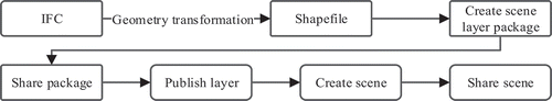
Before the transformed shapefile models can be used by the bridge management system, they need to be properly managed online. The workflow for data processing and online data management is represented in Figure 9. The IFC file is first transformed into shapefile, which is later turned into a scene layer package using ArcGIS Pro. The layer package will then be uploaded to and managed by ArcGIS Online. To improve efficiency, this process has been automated using the data processing model builder of ArcGIS Pro.

Figure 9. Workflow for online data management

4.2.2. Structure of the system

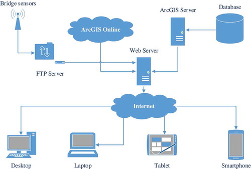
Figure 10 shows the physical structure of the developed system. It requests data from several sources, including ArcGIS Online, ArcGIS Server, and an FTP Server for real-time sensor data. This system is deployed on a Web Server, which can then be accessed by various end clients such as desktops, laptops, tablets, and smartphones through the Internet.

Figure 10. Physical structure of the system

Three functions have been realized in this system, including optimized visualization by combining 2D and 3D views, model exploration, and real-time sensor data reception and visualization.

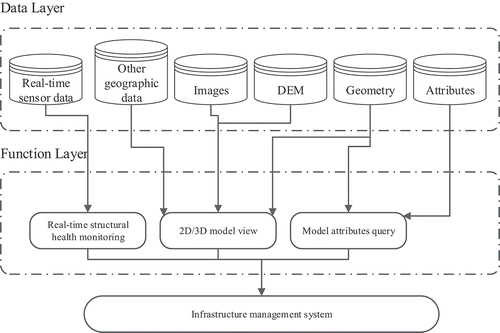
Figure 11 represents the logical structure of the system, revealing the connections between data input, functions, and system. Two layers, i.e., data layer and function layer, are included in the system. In addition, real-time sensor data are used to simulate real-time structural health monitoring process, since a real real-time steam was not available. Images, DEM, the geometry of BIM models, and other geographic data are used in the 2D/3D view. The geometry and attributes of BIM models can be used in information queries.

Figure 11. Logical structure of the system

During the simulation of real-time structural health monitoring, a two-minute event dataset provided by Main Roads Western Australia was used. The simulation is realized by three steps: (a) transforming event data from EXCEL (.xls) into JavaScript Object Notation (JSON) using a MATLAB script, (b) setting up a server and saving the JSON file in the server, and finally (c) requesting the JSON file from the client. A server has to be used to host the JSON file, because the security mechanisms of most browsers, such as Firefox and Chrome, do not allow a JSON file to be accessed from a local directory.

4.2.3. User interface of the system

The developed system interface (Figure 12) contains five sections, including navigation tools, background selection tool, model display, sensor data visualization, and entity list.

Figure 12. User interface of the system

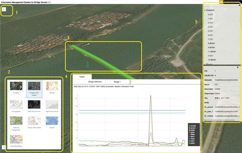
(a) Navigation tools control the orientation of the scene and allow the user to return to the default view through just one click. (b) The background selection tool allows switching between various background maps, such as imagery, topography. (c) Model display is the main section for displaying models, occupying much of the interface. (d) The status panel is designed for the visualization of sensor data. Finally, (e) the entity list is used to show all elements and their attributes, such as global ID, name, tag, and so on.

The features that distinguish this system include (a) an advanced visualization combining 2D and 3D views; and (b) real-time sensor data reception, allowing sensor data to be received and visualized in a real-time manner.

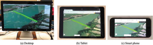
Figure 13 shows the system running on different end clients, including desktop, tablet, and smartphone. This system is currently designed for use on desktops and laptops with large screens. It can also be run on tablets or smartphones with small screens, but this is not recommended at present.

Figure 13. System running on (a) desktop, (b) tablet and (c) smartphone

5. Discussion

5.1. Entities not closed

The transformed bridge model is examined by the $IsClosed$ tool of ArcGIS, which checks whether the topology of each geometry is closed (solid modelling). Unfortunately, not all entities are closed, such as those for member and slab. Table 5 represents the results.

Table 5. Quantity of closed geometry for each element and percentage

	Memory-16GB	Memory-32GB
Beam	195 (100%)	195 (100%)
Column	11 (100%)	11 (100%)
Footing	6 (100%)	6 (100%)
Member	147 (38.7%)	220 (57.9%)
Slab	15 (93.8%)	16 (100%)
Total	374 (61.5%)	448 (73.7%)

Two machines were used in the examination, one with 16GB memory and the other with 32GB memory, after it is found that this problem may be related to the memory capacity. Using the same script, when increasing the memory to 32GB, the number of closed geometries increases to 448 from 374. This issue can be addressed using the $EncloseMultipatch$ tool, and the processing time would largely depend on the quantity and complexity of the geometry being processed.

5.2. Limitations and future work

The main limitations and future work of this study are listed as follows:

1. BIM models contain two types of information, i.e., geometric and semantic information. This study mainly focuses on the transformation of geometry, and semantic information is not fully transferred. Only the essential attributes, such as element ID and element type, are transferred. In the future, a method for thorough semantic information transfer to GIS is needed.

2. The system developed in this study is, by far, a prototype and is mainly used for visualization of the bridge model and the real-time bridge structure health monitoring data. The user interface and functions are quite limited and need to be further improved. For example, more advanced analysis functions, such as predictive building maintenance, may be realized by incorporating data mining, artificial intelligence, and so on.

3. New method for geometry conversion should be explored, such as using Open CASCADE. As mentioned before, Open CASCADE has been used in 3D object conversion and visualization in areas such as CAD, CAE and CAM. In the future, this approach should be studied and compared with the method presented in this paper.

6. Conclusions

This paper aims at transforming BIM models in IFC format into GIS models in shapefile format. The commonly used profiles for swept solid, such as rectangle profile, circle profile, arbitrary profile and I-shape profile, are investigated, and algorithms have been developed to transform swept solid into Brep. A bridge model is then used to validate the proposed method and a Web GIS-based bridge management system is developed to show a potential usage of the transformed shapefile bridge model. The main findings and outcome of this study include that the proposed method can transform IFC models to shapefile models; however, the geometry of some components may not be closed; in the future, the functionality of the developed bridge management system should be further improved.

BIM/GIS integration is attracting attention from both the geospatial industry and AEC/FM domain. This study has demonstrated a systematic process of BIM/GIS integration, from the beginning data conversion to the end application using a bridge model. Its contribution is twofold. First, the process and approach of transforming BIM components into usable data in a GIS environment are developed. Compared with previous studies, this process and approach can be achieved in an easy and reliable way. In addition, the integration of BIM and GIS has been applied to bridge management, considering the fact that studies on the application of this technique are currently confined to a small number of areas, such as fire response management, traffic noise assessment, flood damage assessment and indoor route planning.

Disclosure Statement

No potential conflict of interest was reported by the authors.

Additional information

Funding

This work was supported by the Australian Research Council [#DP170104613,#DP180104026] and by the Shanghai Economic and Information Commission Special Fund Programs, grant number: Shanghai J-2018-27..

References

- Amirebrahimi, S., A. Rajabifard, P. Mendis, and T. Ngo. 2016a. “A BIM-GIS Integration Method in Support of the Assessment and 3D Visualisation of Flood Damage to A Building.” Journal of Spatial Science 61 (2): 317–350. doi:10.1080/14498596.2016.1189365.
- Amirebrahimi, S., A. Rajabifard, P. Mendis, and T. Ngo. 2016b. “A Framework for A Microscale Flood Damage Assessment and Visualization for A Building Using BIM–GIS Integration.” International Journal of Digital Earth 9 (4): 363–386. doi:10.1080/17538947.2015.1034201.
- Azhar, S. 2011. “Building Information Modeling (BIM): Trends, Benefits, Risks, and Challenges for the AEC Industry.” Leadership and Management in Engineering 11 (3): 241–252. doi:10.1061/(ASCE)LM.1943-5630.0000127.
- Azhar, S., M. Khalfan, and T. Maqsood. 2015. “Building Information Modelling (BIM): Now and Beyond.” Construction Economics and Building 12 (4): 15–28. doi:10.5130/AJCEB.v12i4.3032.
- Boyes, G. A., C. Ellul, and D. Irwin. 2017. “Exploring BIM for Operational Integrated Asset Management-A Preliminary Study Utilising Real-world Infrastructure Data.” In Paper Presented at the ISPRS Annals of the Photogrammetry, Remote Sensing and Spatial Information Sciences. Melbourne, Australia.
- buildingSMART. 2019. “IfcProfileDef.” Accessed October 29. https://standards.buildingsmart.org/IFC/RELEASE/IFC4_1/FINAL/HTML/
- buildingSMART. 2019a. “IFC Specifications Database.” Accessed October 28. https://technical.buildingsmart.org/standards/ifc/ifc-schema-specifications/
- buildingSMART. 2019b. “IfcIShapeProfileDef.” Accessed February 14. http://www.buildingsmart-tech.org/ifc/IFC2x3/TC1/html/ifcprofileresource/lexical/ifcishapeprofiledef.htm
- Deng, Y., J. C. P. Cheng, and C. Anumba. 2016a. “A Framework for 3D Traffic Noise Mapping Using Data from BIM and GIS Integration.” Structure and Infrastructure Engineering 12 (10): 1267–1280. doi:10.1080/15732479.2015.1110603.
- Deng, Y., J. C. P. Cheng, and C. Anumba. 2016b. “Mapping between BIM and 3D GIS in Different Levels of Detail Using Schema Mediation and Instance Comparison.” Automation in Construction 67: 1–21. doi:10.1016/j.autcon.2016.03.006.
- Eastman, C., P. Teicholz, R. Sacks, and K. Liston. 2011. BIM Handbook: A Guide to Building Information Modeling for Owners, Managers, Designers, Engineers and Contractors. Hoboken, New Jersey: John Wiley & Sons.
- ESRI. 2018. “The Multipatch Geometry Type An Esri White Paper.” Accessed July 31. https://www.esri.com/library/whitepapers/pdfs/multipatch-geometry-type.pdf
- Isikdag, U. 2006. Towards the Implementation of Building Information Models in Geospatial Context. Salford: University of Salford.
- Isikdag, U., S. Zlatanova, and J. Underwood. 2013. “A BIM-Oriented Model for Supporting Indoor Navigation Requirements.” Computers, Environment and Urban Systems 41: 112–123. doi:10.1016/j.compenvurbsys.2013.05.001.
- Li, X., W. Peng, G. Q. Shen, X. Wang, and Y. Teng. 2017. “Mapping the Knowledge Domains of Building Information Modeling (BIM): A Bibliometric Approach.” Automation in Construction 84: 195–206. doi:10.1016/j.autcon.2017.09.011.
- Li, X., G. Q. Shen, W. Peng, and T. Yue. 2019. “Integrating Building Information Modeling and Prefabrication Housing Production.” Automation in Construction 100: 46–60. doi:10.1016/j.autcon.2018.12.024.
- SAS, OPEN CASCADE. 2019a. “BRep Format.” Accessed October 25. https://www.opencascade.com/doc/occt-7.2.0/overview/html/occt_user_guides__brep_wp.html
- SAS, OPEN CASCADE. 2019b. “Be Free with Your 3D Modeling Kernel.” Accessed October 25. https://www.opencascade.com/content/open-source-core-technology
- Tan, Y., Y. Song, J. Zhu, Q. Long, X. Wang, and C. P. Jack. 2018. “Optimizing Lift Operations and Vessel Transport Schedules for Disassembly of Multiple Offshore Platforms Using BIM and GIS.” Automation in Construction 94: 328–339. doi:10.1016/j.autcon.2018.07.012.
- Tashakkori, H., A. Rajabifard, and M. Kalantari. 2015. “A New 3D Indoor/outdoor Spatial Model for Indoor Emergency Response Facilitation.” Building and Environment 89: 170–182. doi:10.1016/j.buildenv.2015.02.036.
- Teo, T.-A., and K.-H. Cho. 2016. “BIM-oriented Indoor Network Model for Indoor and Outdoor Combined Route Planning.” Advanced Engineering Informatics 30 (3): 268–282. doi:10.1016/j.aei.2016.04.007.
- Volk, R., J. Stengel, and F. Schultmann. 2014. “Building Information Modeling (BIM) for Existing buildings—Literature Review and Future Needs.” Automation in Construction 38: 109–127. doi:10.1016/j.autcon.2013.10.023.
- Xu, M., I. Hijazi, A. Mebarki, R. E. Meouche, and M. Abune’meh. 2016. “Indoor Guided Evacuation: TIN for Graph Generation and Crowd Evacuation.” Geomatics, Natural Hazards and Risk 7 (sup1): 47–56. doi:10.1080/19475705.2016.1181343.
- Zhu, J., Y. Tan, J. Wang, and X. Wang. 2017. “An Economical Approach to Geo-referencing 3D Model for Integration of BIM and GIS.” Paper Presented at the International Conference on Innovative Production and Construction (IPC 2017). Perth. 30 Nov - 1 Dec.
- Zhu, J., P. Wang, and X. Wang. 2018. “An Assessment of Paths for Transforming IFC to Shapefile for Integration of BIM and GIS.” In Paper Presented at the 2018 26th International Conference on Geoinformatics. Kunming, China.
- Zhu, J., X. Wang, M. Chen, W. Peng, and M. J. Kim. 2019a. “Integration of BIM and GIS: IFC Geometry Transformation to Shapefile Using Enhanced Open-source Approach.” Automation in Construction 106: 102859. doi:10.1016/j.autcon.2019.102859.
- Zhu, J., X. Wang, P. Wang, W. Zhiyou, and M. J. Kim. 2019b. “Integration of BIM and GIS: Geometry from IFC to Shapefile Using Open-source Technology.” Automation in Construction 102: 105–119. doi:10.1016/j.autcon.2019.02.014.
- Zhu, J., G. Wright, J. Wang, and X. Wang. 2018. “A Critical Review on the Integration of Geographic Information System and Building Information Modelling at the Data Level.” ISPRS International Journal of Geo-Information 7 (2): 66. doi:10.3390/ijgi7020066.