Spatiotemporally Varying Coefficients (STVC) model: a Bayesian local regression to detect spatial and temporal nonstationarity in variables relationships

ABSTRACT

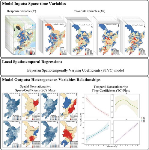
Local regression has an advantage over global regression by allowing coefficients that qualify variables relationships being heterogeneous, where such varying regression relationships are nonstationarity. Spatiotemporally Varying Coefficients (STVC) model is the first Bayesian-based local spatiotemporal regression approach, intending to simultaneously detect spatial and temporal nonstationarity for heterogeneous response-covariate variables relationships, through separately estimating posterior local-scale coefficients over different space areas and time frames. In this paper, we first presented a general Bayesian STVC modelling paradigm as a specification guide to show its commonality in broader geospatial research. Then, we employed it to solve a real-world issue concerning spatiotemporal healthcare-socioeconomic relations, for which we derived data of county-level hospital beds number per capita, as well as data of related socioeconomic factors in northeast China during 2002–2011. Results showed that the STVC model surpassed all the other comparative regressions, in terms of both Bayesian model fitness and predictive ability. Globally, resident savings, financial institutions loans, GDP, and primary industry were identified as key socioeconomic conditions affecting healthcare resources in Northeast China. Temporally, with Time-Coefficients (TC) plots, we found that after 2011, GDP and primary industry would further help improve the overall healthcare level of northeast China. Spatially, with Space-Coefficients (SC) maps, we could directly identify the relative contribution of four socioeconomic covariates’ impacts on healthcare within each administrative county. Bayesian STVC model is an essential development and extension of the local regression family for exploring the spatiotemporal heterogeneous variables relationships, especially under Bayesian statistics, as well as GIScience and spatial statistics.

Graphic abstract

KEYWORDS:

• Bayesian STVC
• local spatiotemporal regression
• spatiotemporal nonstationarity
• heterogeneous variables relationships
• China’s healthcare and socioeconomic

1. Introduction

Geospatial data usually do not fit traditional, non-spatial regression requirements due to two cornerstones of spatial characteristics, namely, spatial autocorrelation (dependence) (Dale and Fortin 2002; Tobler 1970; Anselin and Griffith 1988) and spatial heterogeneity (Goodchild 2004b; Anselin 1990). Two spatial characteristics are playing fundamental roles in Geographic Information Science (GIScience) (Goodchild 2004a), spatial statistics and econometrics, as well as modern geospatial big data analysis in multidisciplinary fields (Gelfand et al. 2010; Haining and Haining 2003). One of the main objectives in geospatial analysis is to determine the relationships that exist between different variables (Brunsdon, Fotheringham, and Charlton 1996; Fotheringham, Charlton, and Brunsdon 1996). Spatial regression is the most widely utilized and accepted statistical technique to quantify variables relationships by considering the aforementioned two underlying spatial data characteristics.

Generally, spatial regression could be classified into two categories, global spatial regression and local spatial regression (Wolf, Oshan, and Fotheringham 2018). The classification is based on a regression process whether incorporates the spatial heterogeneity in regression relationships (i.e., explanatory variables whose impacts on the outcome of interest vary throughout geographic space), or only considers a constant regression relationship (Fotheringham, Brunsdon, and Charlton 2003). Nonstationarity is commonly utilized to describe the heterogeneous relationships between variables in the field of statistics (Brunsdon, Fotheringham, and Charlton 1996; Fotheringham, Charlton, and Brunsdon 1996). In other words, within a regression frame, spatial nonstationarity appears as the local regression coefficients are being varied across the space dimension.

Global spatial regression models, such as conditional autoregressive model (CAR) (Besag 1974) and simultaneously autoregressive model (SAR) (Whittle 1954), are considered to be effective methods to account for the spatial autocorrelation of the response variable into modelling, but not for incorporating spatial nonstationarity among covariate variables, which can lead to under-fitting and insufficient explanatory issues, especially for large-domain and fine-scale geospatial studies (Brunsdon, Fotheringham, and Charlton 1996; Fotheringham, Charlton, and Brunsdon 1996).

Beyond global spatial regression, local spatial regression overcomes aforementioned issues by further taking the spatial heterogeneity of variables relationships into account, among which the two most widely accepted and frequently encountered models are the frequentist Geographically Weighted Regression (GWR) model (Brunsdon, Fotheringham, and Charlton 1996; Fotheringham, Charlton, and Brunsdon 1996) and the Bayesian Spatially Varying Coefficient (SVC) model (Gelfand et al. 2003; Banerjee, Carlin, and Gelfand 2014). Both GWR and SVC models are based on the same underlying assumption and enable similar analyses by producing very similar results in terms of local parameters. Nevertheless, under different statistical frameworks, their estimators are quite different (Wolf, Oshan, and Fotheringham 2018; Waller et al. 2007). In contrast to frequentist methods, Bayesian methods provide uncertainties as credible intervals on parameters that are in line with common sense interpretations. In addition, Bayesian methods with prior beliefs could handle complex models that are difficult to fit using classical methods (Wang, Ryan, and Faraway 2018; Moraga 2019).

Specifically, compared with Bayesian SVC, GWR is much easier formulated using the language of ordinary regression and has been shown to be more robust in larger samples (Páez, Farber, and Wheeler 2011; Fotheringham and Oshan 2016). However, GWR is a data-borrowing method limited to its inferential scope (Finley 2011), not a full-map model using a complete and unified modelling strategy, thus highly sensitive to the choice of the bandwidth (Wolf, Oshan, and Fotheringham 2018). On the contrary, the full-map Bayesian SVC model not only overcomes above issues but also has flexible modelling advantages with a hierarchical specification that can extend it to many settings (Finley 2011; Blangiardo and Cameletti 2015). In addition, the precious research further suggested that Bayesian SVC produced more accurate estimates of regression coefficients than GWR, particularly in the presence of collinearity (Wheeler and Calder 2007; Wheeler and Waller 2009; Finley 2011). However, the increased flexibility of Bayesian SVC model comes at a cost by suffering from the computational burden, which is a common issue among all Bayesian-based local regressions, due to its much higher model complexity arising from the crude Bayesian modelling (Bolker 2009; Finley 2011; Waller et al. 2007). For example, the computing time of Bayesian SVC was 466 and 1286 times than that of a GWR for two independent data sets, in a recent controlled study using Markov Chain Monte Carlo (MCMC) as the Bayesian inference algorithm (Wolf, Oshan, and Fotheringham 2018). Nonetheless, with the fast improvement of the Bayesian inference algorithm during the last decade, the in-situ computational burden from Bayesian modelling seems to be acceptable at present (Rue, Martino, and Chopin 2009; Rue et al. 2017; Ugarte et al. 2014).

Currently, only GWR has developed its space-time type model within the frequentist frame, namely, geographically and temporally weighted regression (GTWR) (Fotheringham, Crespo, and Yao 2015; Huang, Wu, and Barry 2010), which has gained attention and development recently (Wu et al. 2019; Liu et al. 2017). However, under the Bayesian statistics frame, after SVC, no such Bayesian-based local spatiotemporal regression has been officially proposed and named yet. The foremost top-drawer challenge is that such Bayesian-based local spatiotemporal regression must have the ability and potential to be applied to large-scale geospatial big data, which requires the normal modelling form (model complexity) of it should not be too complicated, mainly considering the inevitable issues arising from the in-situ Bayesian hierarchical modelling (BHM) strategy (Finley 2011; Choi et al. 2012). The first issue is the computing burden from the booming growth of the model complexity of Bayesian-based local spatiotemporal regressions, which hinders the widespread use of such models for general practitioners with limited hardware resources. The second issue is trickier and only exists in the Bayesian-based models because of its full-map modelling strategy, which herein is named as the too-local-to-model (TLTM) problem, rooting in the strict criterion of Bayesian model evaluation. Specifically speaking, when the modelling scenario is for a big space-time multivariable data, a mostly local-scale Bayesian spatiotemporal regression, also being with the highest space-time model complexity, can lead to a far worse model performance representing the model is not usable at all, due to the local errors in every individual space-time units will be magnified when they are summarized, thus affecting the whole. One way to solve the Bayesian model complexity issues is to sharply reduce the spatial resolution/scale (Choi et al. 2012), but giving away the original fine-scale geospatial information and adding additional uncertainties from spatial grouping, which is definitely not an ideal solution in today’s era of big data.

To fill this gap in local regression family, we proposed the Spatiotemporally Varying Coefficients (STVC) model, a first Bayesian-based local spatiotemporal regression, to simultaneously detect the spatial and temporal nonstationarity in heterogeneous response-covariate variables relationships, by taking advantages of both Bayesian statistics theories and hierarchical modelling framework, as well as separately estimating posterior local-scale regression coefficients to vary across space and over time (Song et al. 2019a). The Bayesian STVC model turns out to be a feasible prototype for relatively larger-scale space-time data, supported by a real-world epidemiological hand, foot, and mouth disease case. Besides the differences between a frequentist GWR and a Bayesian SVC model aforementioned, compared with the frequentist GTWR model (Fotheringham, Crespo, and Yao 2015; Huang, Bo, and Barry 2010), the Bayesian STVC model separately fits the space and time dimension parameters to weak the in-situ model complexity issues of BHM in local spatiotemporal regression, which are also very practical for applied users to directly generalize the spatial and temporal regularities to mine the mechanism behind the objective phenomenon of interest. Moreover, like mixed GTWR (Liu et al. 2017), the Bayesian STVC model is also a mixed regression model that is capable of synchronously capturing the global-scale stationarity and the local-scale spatiotemporal nonstationarity in variables relationships.

However, as a newly proposed approach, the underlying theories of Bayesian STVC modelling need to be further clarified and improved in a generally utilized way, as well as verified by more examples. The following part of this paper is structured as below. Section 2 comprehensively introduces the settings and principles of a general Bayesian STVC model. Section 3 applies a hands-on real-world case to explore the spatiotemporal healthcare-socioeconomic relations in northeast China, also to test the Bayesian STVC model by comparing it with other mainstream models. Section 4 discusses the advantages, limitations, as well as prospects of Bayesian STVC modelling. Section 5 summarizes the contributions of this work.

2. Statistical methods

2.1 A general Bayesian STVC model

The Spatiotemporally Varying Coefficients (STVC) model is a Bayesian-based local spatiotemporal regression approach, aiming at detecting the heterogeneous response-covariate variables relationships (nonstationarity) in both spatial and temporal dimensions (Song et al. 2019a). The formulas of a general Bayesian STVC model are illuminated with equations (1)(1) ${\eta }_{it}=g(y_{it}\in Y)$(1) – (4(4) $\gamma =({\gamma }_1,\dots ,{\gamma }_T{)}^{\prime }\sim \mathrm{N}(0,{\sigma }_{\gamma }^2{Q}_{\gamma }),Q_{\gamma }={\mathrm{M}}_{\gamma }^{-}$(4) ) in sequence, designed to be applied for broader geospatial-related research.

(1) ${\eta }_{it}=g(y_{it}\in Y)$(1)

(2) ${\eta }_{it}=\alpha +\sum _{k=1}^{K}f({\mu }_{k,i}Xk,it)+{\displaystyle \sum _{k=1}^{K}f({\gamma }_{k,t}{X}_{k,it}})+{\displaystyle \sum _{h=1}^H{\beta }_h{C}_{h,it}}+f({\xi }_i)+f({\psi }_t)$(2)

(3) ${\eta }_{it}=\alpha +\sum _{k=1}^{K}f({\mu }_{k,i}Xk,it)+{\displaystyle \sum _{k=1}^{K}f({\gamma }_{k,t}{X}_{k,it}})+{\displaystyle \sum _{h=1}^H{\beta }_h{C}_{h,it}}+f({\xi }_i)+f({\psi }_t)$(3)

(4) $\gamma =({\gamma }_1,\dots ,{\gamma }_T{)}^{\prime }\sim \mathrm{N}(0,{\sigma }_{\gamma }^2{Q}_{\gamma }),Q_{\gamma }={\mathrm{M}}_{\gamma }^{-}$(4)

Equation (1)(1) ${\eta }_{it}=g(y_{it}\in Y)$(1) represents the data likelihood model, where space-time observations $y_{it}$ are the values of the target response variable of interest Y in space i and time t, ${\eta }_{it}$ are the structural additive predictors. $g(\cdot )$ is the likelihood function that is utilized to link ${\eta }_{it}$ and $y_{it}$, which can be seen as the prior distribution of Y, and in many situations, assumed to belong to an exponential family (Wang, Ryan, and Faraway 2018).

Equation (2)(2) ${\eta }_{it}=\alpha +\sum _{k=1}^{K}f({\mu }_{k,i}Xk,it)+{\displaystyle \sum _{k=1}^{K}f({\gamma }_{k,t}{X}_{k,it}})+{\displaystyle \sum _{h=1}^H{\beta }_h{C}_{h,it}}+f({\xi }_i)+f({\psi }_t)$(2) represents the space-time process model that is the core design of an STVC, in which the structured linear predictor ${\eta }_{it}$ accounts for various effects of covariates in an additive way. Generally, the posterior estimated parameters can include six components in total. Among them, ${\beta }_h$, ${\mu }_{k,i}^{\hspace{0.17em}}$ and ${\gamma }_{k,t}^{\hspace{0.17em}}$ are the covariates’ coefficients, which represent the global-scale stationary, local-scale spatial and temporal nonstationary effects in variables relationships. Similarly, $\alpha$, ${\xi }_i$ and ${\psi }_t$ are the global-scale intercept, and local-scale spatial and temporal intercepts, respectively. The term $X_k$ represents the K main explanatory covariate variables with nonstationary random effect assumption, indicating the coefficients $X_k$ could be varying across space and over time. The term $C_h$ represents the H control covariate variables with stationary fixed effect assumption, which suggests that their coefficients are homogeneous over space and time, and dispensable. Generally, $C_h$ are those covariates with a lesser explanatory contribution to Y, or with no variation either at space or time scale.

Specifically, $\alpha$ and ${\beta }_h$ are the global-scale fixed effect parameters, quantifying the mean intercept and the h-th control covariate’s coefficient. The other four components are all the local-scale random effect parameters including spatial and temporal coefficients ${\mu }_{k,i}^{\hspace{0.17em}}$ and ${\gamma }_{k,t}^{\hspace{0.17em}}$ for the main covariates $X_k$, as well as spatiotemporal intercepts ${\xi }_i$ and ${\psi }_t$. One by one, ${\mu }_{k,i}^{\hspace{0.17em}}$ are the local-scale Space-Coefficients (SC) of the k-th main covariate X, which represent the spatial response-covariate relationships across space areas. ${\gamma }_{k,t}^{\hspace{0.17em}}$ are the local-scale Time-Coefficients (TC) of the k-th main covariate, which represent the temporal response-covariate relationships over periods of time. Similarly, ${\xi }_i$ are the local-scale Space-Intercepts (SI) representing the original spatial structured variation of the response variable Y itself, and ${\psi }_t$ are the local-scale Time-Intercepts (TI) representing the original temporal structured variation of the response variable Y itself.

The random effect components SC and TC are capable of measuring the response-covariate relationships over space and time dimensions, which are the two fundamental outputs from a Bayesian STVC model. The explanation of a local-scale parameter of SC or TC is similar to that of an ordinary global-scale coefficient, which also represents the direction (positive or negative) and strength (absolute value) of a covariate’s relative contribution, with 0 as the threshold value, but in each space or time unit. For instance, a local-scale coefficient for a spatial or temporal unit being greater than 0 indicates that the spatial or temporal effects of the target phenomena are positively associated with a covariate, and the higher the local-scale coefficient, the higher the relative contribution. If the value of a local-scale coefficient is lesser than 0, then the explanation is the opposite.

Moreover, function f () denotes a variety of sub-level latent Gaussian models (LGM) (Rue, Martino, and Chopin 2009; Rue et al. 2017) that can be employed to approximate the spatial and temporal random effects to estimate the locally varying parameters aforementioned (Blangiardo and Cameletti 2015). A combination of these sub-level spatial and temporal LGMs is achieved within the Bayesian hierarchical modelling (BHM) framework (Ugarte et al. 2014; Wang, Ryan, and Faraway 2018) that is introduced in Section 2.2. Herein, we focus on setting f () to account spatial and temporal nonstationary random effects in covariates, which are the distinctive characteristics of the STVC model.

Equation (3)(3) ${\eta }_{it}=\alpha +\sum _{k=1}^{K}f({\mu }_{k,i}Xk,it)+{\displaystyle \sum _{k=1}^{K}f({\gamma }_{k,t}{X}_{k,it}})+{\displaystyle \sum _{h=1}^H{\beta }_h{C}_{h,it}}+f({\xi }_i)+f({\psi }_t)$(3) represents the spatial LGM model that is utilized to fit the spatial structured random effects of SC. To be specific, the STVC model assumes an intrinsic conditional autoregressive (iCAR) prior (Besag 1974) as the spatial LGM model to consider a spatial autocorrelated random effect term to estimate posterior SC for main covariates $X_k$. In equation (3)(3) ${\eta }_{it}=\alpha +\sum _{k=1}^{K}f({\mu }_{k,i}Xk,it)+{\displaystyle \sum _{k=1}^{K}f({\gamma }_{k,t}{X}_{k,it}})+{\displaystyle \sum _{h=1}^H{\beta }_h{C}_{h,it}}+f({\xi }_i)+f({\psi }_t)$(3) , we specified the distribution of ${\mu }_i$ conditional on the set ${{\mu }_{-}}_i={\mu }_{j\ne i}=\left\{{\mu }_1,\dots ,{\mu }_{i-1},{\mu }_{i+1},\dots ,{\mu }_n\right\}$, then the conditional distribution of ${\mu }_i$ is given (Osei, Stein, and Ofosu 2019; Bakka et al. 2018), where ${w_i}_j$ is a spatial proximity matrix, ${w_i}_j=1$ if i and j are neighbours i ~ j (e.g., sharing a common boundary in this case), and 0 otherwise. The mean of the joint prior distribution $\rho ({\mu }_i\left|{\sigma }_{\mu }^2\right.)$ is therefore set to zero with precision matrix ${\sigma }_{\mu }^{-2}{Q}_{\mu }$, where $Q_{\mu }$ is a structural matrix deduced from the binary proximity matrix ${w_i}_j$. The structural matrix $Q_{\mu }$ has diagonal elements $Q_{ii}={\sum }_j{w}_{ij}$ and off-diagonal elements ${Q_i}_j=-w_{ij}$.

Equation (4)(4) $\gamma =({\gamma }_1,\dots ,{\gamma }_T{)}^{\prime }\sim \mathrm{N}(0,{\sigma }_{\gamma }^2{Q}_{\gamma }),Q_{\gamma }={\mathrm{M}}_{\gamma }^{-}$(4) represents the temporal LGM model that is utilized to fit the temporal structured random effects of TC. Concretely speaking, by considering temporal autocorrelation, the STVC model estimates posterior TC for covariates $X_k$ via a structured temporal LGM model dynamically using a neighbouring structure, i.e., the random walk (RW) model that is expressed in equation (4)(4) $\gamma =({\gamma }_1,\dots ,{\gamma }_T{)}^{\prime }\sim \mathrm{N}(0,{\sigma }_{\gamma }^2{Q}_{\gamma }),Q_{\gamma }={\mathrm{M}}_{\gamma }^{-}$(4) , where ${\mathrm{M}}_{\gamma }^{\hspace{0.17em}}$ could be determined by the temporal structure matrix of a first order or second order of RW (Ugarte, Adin, and Goicoa 2016; Blangiardo et al. 2013).

Lastly, the STVC model treats the intercept term either as a global variable or local spatiotemporal variables, depending on whether it is to be fixed or varying over space and time. In terms of fitting spatiotemporal intercepts ${\xi }_i$ and ${\psi }_t$, we could follow the common settings of the mainstream space-time models (Blangiardo and Cameletti 2015; Blangiardo et al. 2013; Ugarte et al. 2014). Herein, following the estimation for SC and TC components, we can also employ the same prior LGMs to estimate posterior SI and TI components, i.e., ${\xi }_i\sim iCAR(Q_{\xi },{\sigma }_{\xi }^2)$ and ${\psi }_t\sim RW(0,{\sigma }_{\psi }^2{Q}_{\psi })$.

2.2 Bayesian hierarchical modelling framework

The proposed STVC model is achieved within the BHM framework that is often used to model spatiotemporal data by allowing complete flexibility in how estimates consider random effects across space and time, and improve estimation and prediction of the underlying features of the model (Blangiardo and Cameletti 2015; Wang, Ryan, and Faraway 2018; Moraga 2019). For a BHM-based STVC model, there are three main levels with each level further containing several sub-levels. At the first data distribution level, we employ various likelihood functions to suit different response data distribution, e.g., logistic, binomial, Gaussian (Wang, Ryan, and Faraway 2018), or even zero-inflated Poisson and negative binomial model (Song et al. 2018b). At the second space-time process level that is the core implementation of an STVC model, we incorporate GLMs of iCAR and RW to account for the spatial and temporal random effects for vital explanatory covariates with nonstationary assumption. At the third parameter level, we specify non-informative priors for the parameters and their variance components, which allowed the large-scale geospatial observed data to have the greatest influence on posterior distributions (Schrödle and Held 2011; Wang, Ryan, and Faraway 2018). One of the main advantages of utilizing BHM is its extra flexible modelling frame, allowing stakeholders to customize advanced statistical models (Yang et al. 2019; Blangiardo and Cameletti 2015; Wang, Ryan, and Faraway 2018).

2.3 Bayesian model inference and evaluation

The integrated nested Laplace approximation (INLA) computational approach (Rue, Martino, and Chopin 2009) was adopted to perform approximate Bayesian inference in LGMs using the R package INLA, for estimating posterior parameters of the BHM-based STVC model and other comparative models of this study. The main reason is that the INLA algorithm has the advantage of relatively short computation time with accurate parameter estimates, ad hoc for estimating LGMs (Bakka et al. 2018; Rue et al. 2017; Ugarte et al. 2014). Three criteria, model fitness, model complexity, and model predictive ability, are utilized to assess and compare Bayesian models (Blangiardo et al. 2013; Song et al. 2019b). First, Bayesian model fitness is quantified by two indices Deviance Information Criterion (DIC) (Spiegelhalter et al. 2002) and Watanabe Akaike Information Criterion (WAIC) (Watanabe 2010). The indicators of DIC and WAIC are both the smaller, the better. Then, Bayesian model complexity is quantified by indices of effective parameters (P_DIC and P_WAIC) that are obtained with DIC and WAIC methods synchronously. Higher values of P_DIC and P_WAIC indicate a more complex model. Finally, Bayesian model predictive ability is quantified by a logarithmic score (LS) that is extracted from the conditional predictive ordinates under a leave-one-out cross-validation, which is the smaller, the better (Held, Schrödle, and Rue 2010).

3. Empirical case study

3.1 Study topic

Geospatial distribution of healthcare resources is an important dimension of healthcare access, where healthcare resources clustered or missing in a certain region commonly cause geospatial inequalities, which no longer meet the actual needs of civilians (Shi and Kwan 2015; Shi and Wang 2015). In China, the healthcare inequality issue is noteworthy in the geospatial dimension and serious at a finer scale (Li and Dennis Wei 2010; Wang and Pan 2016). Most previous studies of China’s healthcare resources were focused at the entire country-level or regional province-level (Li and Wei 2014; Zhang et al. 2015; Lu and Zeng 2018) but seldom at the administrative county level (Pan and Shallcross 2016).

Our literature review showed that in China, socioeconomic conditions play an important role in affecting hospital beds resources and is a key indicator reflecting healthcare resources, e.g., GDP, financial expenditure, population size (Qin and Hsieh 2014; Guo and Luo 2019); residents’ saving, government revenue (Pan and Shallcross 2016); elderly population, urban population proportion, and healthcare expenditure (Ye et al. 2018). However, previous research did not consider a comprehensive factors system covering diverse socioeconomic aspects related to hospital beds resources at the finest county-level scale.

Previous studies commonly assumed that the healthcare-socioeconomic relationships were homogeneous over the entire area and time frame, based on a global-scale stationary assumption (Lu and Zeng 2018; Pan and Shallcross 2016). However, it is more reasonable that the real-world healthcare-socioeconomic relationships are heterogeneous at both spatial and temporal scales under a spatiotemporal nonstationary assumption, especially for a large-scale geospatial study. However, regarding China, such heterogeneous healthcare-socioeconomic relationships have only been discussed in the spatial dimension (Ye et al. 2018; Li and Wei 2014; Wu et al. 2016). There are no studies in China that have investigated both the local-scale spatial and temporal nonstationary impacts of various socioeconomic factors on healthcare resources equalities so far. These studies may offer new insights into formulating multi-level administrative policies.

3.2 Data sources and processing

To solve the aforementioned issues and to test the practicability of the Bayesian STVC model, we used data of the yearly hospital beds number per 10,000 people as the target variable of interest representing the county-level healthcare resources condition across northeast China from 2002 to 2011. Correspondingly, we collected a total of 20 socioeconomic variables as the potentially county-level influencing factors of healthcare resources over the study area during the same period (Supplementary file, Table S1). Both the response and covariate variables were retrieved from a published China’s county-level official socioeconomic statistics dataset, which was originally collected from the China County Statistical Yearbook, the China Statistical Yearbook for Regional Economy, and the China City Statistical Yearbook (Song et al. 2018a).

Descriptive statistics of the modelling data including both the response and covariate variables are summarized in supplementary file S2 (Table S2). Based on the results, we employed the z-score standardization method to process all of the twenty socioeconomic covariates with different units to make them dimensionless, and we set the response variable of healthcare resources to follow a prior data distribution model of log Gaussian likelihood function, to approximate a normal distribution.

Regarding further regression modelling, we employed the variance inflation factor (VIF) to exclude socioeconomic covariates with higher multicollinearity (VIF>10) (Bo et al. 2014) and further utilized the random forest method to select the core covariates with higher relative importance and contribution for improving model fitness (Genuer, Poggi, and Tuleau-Malot 2010). An introduction of VIF and random forest, as well as the detailed selection experiment of twenty socioeconomic covariates, are summarized in Supplementary file S2 (Table S3, and Figure S1). As a result, the final selected four socioeconomic covariate variables were X1 balance of urban and rural resident’s savings per capita, X2 balance of loans from financial institutions per capita, X3 GDP (gross domestic product) per capita, and X4 primary industry output value per capita.

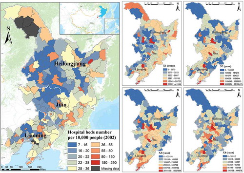
Figure 1(a) illustrates the study area and the county-level map of the response variable (hospital beds per 10,000 people) in the year 2002. Moreover, we presented maps of four socioeconomic covariate variables in the same period in Figure 1(b-e) respectively.

Figure 1. Experimental data in the study area of northeast China at the county level in the year 2002: (a) response variable: hospital beds per 10,000 people; socioeconomic covariate variables: (b) X1 balance of urban and rural resident’s savings per capita, (c) X2 balance of loans from financial institutions per capita, (d) X3 GDP per capita, and (e) X4 primary industry output value per capita.

3.3 Models implementation

As a comprehensive evaluation, we compared the advanced STVC model with the other four benchmark regressions under the BHM framework, following a prior data distribution of log Gaussian likelihood. Socioeconomic variables X1-X4 were selected as the core covariates in regression modelling. Supplementary file S3 gives detailed formula specifications of the above five regression models. Briefly, model 1 was an ordinary multivariable regression, only with the stationary fixed effects of covariates. Model 2 was a spatiotemporal multivariable regression considering both spatiotemporal random effects of intercepts and covariates’ fixed effects. Model 3 was an SVC regression, only accounting for the spatial nonstationary random effects of covariates, while model 4 was a Temporally Varying Coefficients (TVC) regression, only accounting for the temporal nonstationary random effects of covariates. Finally, model 5 was a customized STVC model without incorporating spatiotemporal intercepts, to avoid the local influences of intercepts on estimating nonstationary response-covariates relationships.

Table 1 summarizes the results of the Bayesian model evaluation of five comparative regressions using five mainstream indicators. With the lowest DIC, WAIC, and LS values, the newly proposed STVC model (model 5) is the best in terms of both model fitness and predictive ability. STVC model is better than both SVC and TVC, suggesting the effectiveness of synchronously considering spatial and temporal nonstationarity in covariates. The complexity (P_DIC and P_WAIC) of model 5 is vastly higher than an ordinary multivariable regression (model 1) and even 1.872 times that of a spatiotemporal multivariable regression (model 2). Nevertheless, the increase in the complexity of STVC modelling is rewarding due to two benefits. Firstly, the STVC model achieves the best model performance, even without considering the spatiotemporal random effects of intercepts. Secondly, only the STVC model can estimate local-scale varying coefficients for further analysing the spatial and temporal heterogeneous response-covariates relationships, i.e., healthcare-socioeconomic relationships.

Table 1. Evaluation of five comparative Bayesian regression models accounting for model fitness, complexity, and predictive ability.

Models	DIC	WAIC	PDIC	PWAIC	LS
model 1	16060	16115	5.83	56.51	4.46
model 2	11083	11089	188.18	177.39	3.07
model 3	11368	11351	288.34	229.74	3.16
model 4	14876	14917	37.03	69.28	4.13
model 5	10935	10920	469.94	375.07	3.06

Note DIC deviance information criterion; WAIC Watanabe-Akaike information criterion; P_DIC effective number of parameters for DIC; P_WAIC effective number of parameters for WAIC; LS logarithmic score; model 1–5: ordinary multivariable, spatiotemporal multivariable, SVC, TVC, and STVC regression models.

3.4 Time-Coefficients (TC) visualization

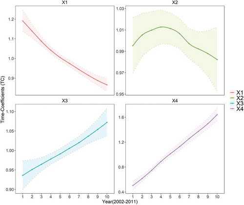
The first fundamental outputs of a Bayesian STVC model were the TC plots for measuring the temporal nonstationary effects of each socioeconomic covariate (variables X1-X4) on the response variable (healthcare resources), as shown in Figure 2. The temporal associations were not consistent, but with both linear and nonlinear trends over 2002–2011, indicating the necessity of incorporating the temporal nonstationary random effects in regression modelling. Generally, we discovered that only covariates X3 and X4 showed an upward trend throughout ten years, while all the other covariates (X1 and X2) showed downward trends. To be specific, for the first five years, X1 and X2 may play more important roles in developing healthcare resources in northeast China, while for the last five years, the influences of X3 and X4 on healthcare resources became more imperative. After 2011, efforts to develop the regional economy (X3), especially the primary industry (X4), may help further improve the overall healthcare level in the region of northeast China.

Figure 2. Time-Coefficients (TC) plots for measuring temporal healthcare-socioeconomic relationships during 2002–2011 over northeast China: X1 balance of urban and rural resident’s savings per capita, X2 balance of loans from financial institutions per capita, X3 GDP per capita, and X4 primary industry output value per capita. Dotted lines are the credible intervals representing the upper and lower uncertainties of the estimated TC.

3.5 Space-Coefficients (SC) visualization

The second fundamental outputs of a Bayesian STVC model were the SC maps for measuring the spatial nonstationary effects of four socioeconomic covariates on the response variable of healthcare resources, as shown in Figure 3. We classified the SC values into ten grades to present the spatially varying trends. We further retrieved the hotspot maps based on the corresponding SC maps in Figure 3, to show which regions had significant clusters of high-contribution hot spots (red) and low-contribution cold spots (blue), also which regions were not significant (yellow) indicating that the local coefficients within a region were not statistically significant enough to form a cluster. Supplemental file S4 introduces the underlying theories of a Getis-Ord Gi* statistic-based hot spot analysis for spatial cluster mapping (Ord and Getis 1995).

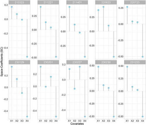
In all SC maps of four socioeconomic covariates, we detected significant spatial clusters, suggesting the necessity of considering spatial autocorrelation in healthcare-socioeconomic nonstationary relations in STVC modelling. In practice, regarding an influencing covariate of interest, we could visually distinguish which local-scale areas were sensitive to this covariate for improving healthcare resources, as well as which areas were not, by directly applying the target SC map of that covariate with Figure 3. More practically, within each administrative county, we could further identify the individually local-scale impacts of four socioeconomic covariates on the outcome of healthcare resources, by vertically integrating the county-level information via all the SC maps together. As illustrated in Figure 4, we selected ten counties randomly as the representatives for producing the SC lollipop charts to express the county-specific spatial nonstationarity.

Furthermore, by using those SC’s hot spot maps, we discovered that personal economic level and financial investment (X1 and X2) were more important in Heilongjiang Province, and GDP, especially the primary industry (X3 and X4) were more important in Jilin Province, but no socioeconomic covariates were significant enough to form a contributing hot spot cluster in Liaoning Province. By combining SC maps with SC’s hotspot maps, it could provide policymakers with multi-level actionable information for the development and implementation of appropriate public health policies.

Figure 3. Space-Coefficients (SC) maps for measuring the county-level spatial healthcare-socioeconomic relationships across northeast China, and their hot spot maps: X1 balance of urban and rural resident’s savings per capita, X2 balance of loans from financial institutions per capita, X3 GDP per capita, and X4 primary industry output value per capita.

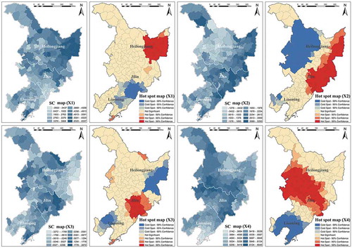
Figure 4. Lollipop charts of Space-Coefficients (SC) to display county-specific associations of healthcare resources with various socioeconomic covariates in ten counties of northeast China (210323, 211221, etc.): X1 balance of urban and rural resident’s savings per capita, X2 balance of loans from financial institutions per capita, X3 GDP per capita, and X4 primary industry output value per capita.

4. Discussion

As a first Bayesian-based local spatiotemporal regression to detect spatiotemporal nonstationarity in variables relationships, the cutting-edge STVC model fills a vital gap in the local regression family (Song et al. 2019a), where frequentist GWR, GTWR, and Bayesian SVC models have gained considerable attention (Brunsdon, Fotheringham, and Charlton 1996; Fotheringham, Charlton, and Brunsdon 1996; Gelfand et al. 2003; Fotheringham, Crespo, and Yao 2015; Huang, Bo, and Barry 2010). In this work, we focus on presenting a generally utilized prototype of Bayesian STVC modelling first, designed to be suitable to broaden geospatial research requiring the local spatiotemporal regression techniques, by covering the local-scale random effects for spatiotemporal covariates’ nonstationarity and spatiotemporal intercepts, as well as the global-scale fixed effects for auxiliary control covariates.

We demonstrate the practicality and effectiveness of the Bayesian STVC model by applying another real-world example on investigating the healthcare-socioeconomic relationships in northeast China. The STVC model surpassed all the other four comparative models in terms of Bayesian model fitness and predictive ability, even without incorporating the spatiotemporal random effects of intercepts. This STVC setting makes sense in particular for the research target is to explore the nonstationary response-covariates relations along with clearer spatial patterns and temporal trends to ultimately explain the mechanism behind the phenomenon of interest, as it removes the potential interactive influences of local intercepts. Nonetheless, with respects to pursuing a forecast result with higher precision as the main purpose, the STVC model may be better to incorporate such spatiotemporal effects of intercepts, same as the mainstream benchmark global-scale spatiotemporal regression models (Blangiardo and Cameletti 2015; Blangiardo et al. 2013; Ugarte et al. 2014)

With regard to the case study of healthcare resources in northeast China, we summarized some practical findings. First, on a global scale, we confirmed that four socioeconomic factors, including resident savings, loans from financial institutions, GDP, and primary industry, were key influencing aspects of affecting the hospital beds resources in Northeast China. The findings were consistent with previous research, for instance, Qin et al. found that GDP and public spending played important roles in accelerating the diffusion of healthcare resources across regions over China (Qin and Hsieh 2014). Pan et al. found that resident savings and government revenue had significant impacts on hospital beds resources over China (Pan and Shallcross 2016). Guo et al. found that GDP, income, and financial expenditure affected the concentration of hospital beds resources in China (Guo and Luo 2019). Generally, the healthcare level of northeast China was jointly affected by the personal economic level (resident savings), financial investment (loans from financial institutions), as well as the regional economic level (GDP, and primary industry).

Second, going beyond the previous studies limited to the socioeconomic stationary impacts (Lu and Zeng 2018; Pan and Shallcross 2016), it is worth mentioning that this empirical case is the first study in northeast China that investigates both spatial and temporal nonstationary effects of various socioeconomic factors on the distribution of county-level healthcare resources inequality, supported by the advanced Bayesian STVC model, which may offer new insights on multi-level government policymaking, as well as further optimizing medical resources allocation.

Temporally, we discovered that only the impacts of the regional economy characterized by GDP and primary industry showed an upward trend throughout ten years, indicating a continuous contribution of the government-led regional economy on promoting healthcare resources, while the temporal impacts of the personal economy and financial investment showed downward trends. This might suggest that the macro-control at the government level had become a key constraint to the development of healthcare resources in northeast China during the last decade.

Spatially, we detected significant clustered regions for all the four healthcare-socioeconomic relationships maps at both county- and province- levels. Particularly, at the county level, we discovered that in different local-scale areal units, the spatially heterogeneous healthcare-socioeconomic relationships were complicated, and the healthcare resources levels were dominated by a single socioeconomic condition or multiple socioeconomic factors (Wu et al. 2016). Thus, based on the relative impacts of different socioeconomic covariates within each administrative county, we could directly give a specific county-level policy proposal on how to improve the healthcare resources level, which was meaningful for precise and optimized allocation of healthcare resources. At the provincial level, we discovered that personal economic level and financial investment were more critical in province Heilongjiang, while GDP, especially the primary industry were more icritical in province Jilin, which might further offer new insights into the provincial government decision making of public health.

Lastly, we discussed some theoretical comparisons between the Bayesian STVC model and the frequentist GTWR model. Despite the STVC and GTWR modelling frameworks were proposed independently under different statistical traditions (Bayesian and frequentist), and are mathematically and logically distinct, they nevertheless have the same goal of detecting the heterogeneous variables relationships (nonstationarity) and generate very similar modelling results in terms of local coefficient estimates (Wolf, Oshan, and Fotheringham 2018).

However, the differences between STVC and GTWR models originated in frequentist and Bayesian statistical estimators, are conspicuous. First, same as the common differences between the local spatial models of Bayesian SVC and frequentist GWR, the Bayesian STVC model is a real full-map, complete and unified local regression approach, incorporate prior knowledge and uncertainties (e.g., credible intervals on parameters) into modelling directly, and is much more flexible in model scalability and extensity, jointly by taking advantages of Bayesian statistics and hierarchical modelling framework (Finley 2011; Waller et al. 2007). Whether a full-map model or not is an essential difference between Bayesian-based and frequentist-based local regression models, because of the rock-bottom differences between the two statistics estimators, even they can produce similar outputs (Wolf, Oshan, and Fotheringham 2018). Besides, despite the response variable is with missing data, the Bayesian-based local regressions still can estimate a complete and continuous map or plot of the local-scale varying coefficients which cannot be directly estimated by the ordinary frequentist-based local regressions, with the help of the prior spatial/temporal LGMs within the BHM framework.

Second, the fundamental difference between the two local spatiotemporal regressions is that the Bayesian STVC model follows a nonstationary assumption of space-time independence, while the frequentist GTWR model follows a space-time interaction nonstationary assumption. Every coin has two sides, the same for the advanced Bayesian statistics. Even with the superiorities of full-map modelling, the BHM strategy has the noticeable computing burden and too-local-to-model (TLTM) issues, particularly for local regressions with larger samples, as mentioned in the first section (Choi et al. 2012). However, for GTWR that is not a full-map model, it does not have the Bayesian TLTM issue, and its complexity is much smaller than a comparable Bayesian model. Thus, unlike GTWR following a most local-scale space-time interaction assumption, the Bayesian STVC model is given a space-time independence assumption, to ensure its normal modelling form is not too complicated, which have the ability and potential to be applied to large-scale geospatial big data.

We summarized the applied characteristics of a Bayesian STVC model based on the fundamental differences in principle. Firstly, from the algorithm, a separate estimation of space-time coefficients greatly reduces the model complexity, computational burden, and weakens the overfitting issue. Unlike GTWR, Bayesian STVC separately fits the space- and time-dimension coefficients for each covariate variable, by taking advantage of the flexible BHM framework. Therefore, the Bayesian STVC model dramatically reduces the number of parameters needs estimating, i.e., N_STVC = (N_space+N_time)×N_covariates, whereas the number of GTWR’s parameters is N_GTWR = (N_space×N_time)×N_covariates. Secondly, for user applications, the Bayesian STVC model individually outputs the Space-Coefficients (SC) maps and Time-Coefficients (TC) plots for each covariate. Stakeholders can intuitively employ such SC maps and TC plots to understand the structured spatial and temporal regularities for further in-depth data mining, without further processing of the newly estimated three-dimensional space-time interaction coefficients, which is still too complex for discovering simple, precise, and regular findings under some circumstances. Thirdly, the Bayesian STVC model with less burden of computing should have more potential for the down-to-earth application of large-scale geospatial big data, if the users are more interested in utilizing a real full-map local regression model by taking advantages of both Bayesian statistics and hierarchical modelling.

To end our discussion, we would like to talk about the limitations and prospects of Bayesian STVC modelling. First of all, Bayesian-based local regression models commonly suffer from the in-situ computational burden of BHM strategy, and thus regarding a large-dimension and fine-scale dataset along with multiple covariates, the Bayesian STVC model still has the noteworthy issue on computing, which can be partially solved by improving computer hardwires or utilizing fast inference algorithms (Villandré et al. 2020). This is the same as the ‘big-N’ problem in spatial statistics that remains an active area of research, especially for Bayesian statistics (Finley 2011). Second, comparing Bayesian STVC and frequentist GTWR should be a promising direction in the future but must under controlled conditions that are not easy to achieve. On the one hand, previous research pointed that the interpretation of the bandwidth parameter measuring the degree of spatial autocorrelation is not transferrable between the two frameworks of Bayesian and frequentist statistics (Wolf, Oshan, and Fotheringham 2018). On the other hand, only using a tiny dataset, which is not an ideal target of big data application, the Bayesian STVC model could be compared with GTWR by incorporating the same space-time interaction nonstationary effects. Our further studies would focus on developing more sophisticated Bayesian STVC-based statistical models with more serviceable outputs to incorporate advanced informative and underlying geospatial properties (Wang, Zhang, and BoJie 2016; Zhu et al. 2018; Moraga et al. 2017), as well as an acceptable complexity for the easy use in mining spatiotemporal big data (Zhu et al. 2020), to ultimately solve the real-world broader issues concerning the complex space-time relationships between variables.

5. Conclusions

In this article, we present a literature review of the theoretical statistical basis on the newly proposed Bayesian Spatiotemporally Varying Coefficients (STVC) model, which is a first Bayesian-based local spatiotemporal regression method to detect spatial and temporal nonstationarity in heterogeneous relationships among variables. A general formula paradigm of Bayesian STVC modelling is introduced in detail for the first time, to provide a guideline for practitioners to develop the custom-built STVC models to solve broader issues in the real world. We further applied the Bayesian STVC model to firstly explore the spatiotemporal heterogeneous relationships between the county-level healthcare resources and various socioeconomic conditions in northeast China for ten years, expanding the limited knowledge of the complex local-scale healthcare equalities. We found that in northeast China, the personal economic level, financial investment, and the regional economic level were jointly affecting the county-level healthcare resources significantly, at both space and time scales. Temporally, we discovered that government macro-control had become a key factor in developing healthcare resources in northeast China during the last decade. Spatially, an immediate outcome of this work was a series of county-level socioeconomic factors’ contribution maps covering the entire northeast China, which should be the first of its kind. Such factors’ contribution maps could help us formulate the specific policy proposal on further reducing the healthcare equalities at both county and province levels. In conclusion, Bayesian STVC modelling is proposed as a new tool for space-time influencing factors analysis to provide potential clues for the spatiotemporal attribution, which should offer new insights into solving similar issues in broader GIScience, spatial statistics, geostatistics, as well as geospatial-related disciplines.

Acknowledgements

The data were initially collected by Beijing Normal University under the guidance of Yanchen Bo and processed by the Spatial Information Technology and Big Data Mining Research Center in Southwest Petroleum University. We appreciate the International association of Chinese professionals in geographic information sciences (CPGIS) and Jiangxi Normal University for holding the frontier forum of Application of GIS analysis in Public Health. We would like to thank the editors and three anonymous reviewers for their constructive comments and valuable suggestions on improving this manuscript.

Disclosure statement

No potential conflict of interest was reported by the authors.

Supplementary materials

Supplemental data for this article can be accessed here

Additional information

Funding

The work was jointly supported by the National Natural Science Foundation of China under Grant No. 41701448, the Science and Technology Program of Sichuan Province under Grant No. 2020YJ0117, the Humanities and Social Sciences Research Fund Project of Southwest Petroleum University under Grant No. 2019RW021, and the State Key Laboratory of Resources and Environmental Information System under Grant No. 201811. The funders had no role in study design, data collection and analysis, decision to publish, or preparation of the manuscript.

References

- Anselin, L. 1990. “Spatial Dependence and Spatial Structural Instability in Applied Regression Analysis.” Journal of Regional Science 30 (2): 185–207. doi:10.1111/j.1467-9787.1990.tb00092.x.
- Anselin, L., and D. A. Griffith. 1988. “Do Spatial Effecfs Really Matter in Regression Analysis?” Papers in Regional Science 65 (1): 11–34. doi:10.1111/j.1435-5597.1988.tb01155.x.
- Bakka, H., H. Rue, G. Fuglstad, A. Riebler, D. Bolin, J. Illian, E. Krainski, D. Simpson, and F. Lindgren. 2018. “Spatial Modeling with R‐INLA: A Review.” Wiley Interdisciplinary Reviews: Computational Statistics 10 (6): e1443. doi:10.1002/wics.1443.
- Banerjee, S., B. P. Carlin, and A. E. Gelfand. 2014. “Hierarchical Modeling and Analysis for Spatial Data: Chapman and Hall/CRC”.
- Besag, J. 1974. “Spatial Interaction and the Statistical Analysis of Lattice Systems.” Journal of the Royal Statistical Society: Series B (Methodological) 36 (2): 192–225. doi:10.1111/j.2517-6161.1974.tb00999.x.
- Blangiardo, M., and M. Cameletti. 2015. Spatial and Spatio-temporal Bayesian Models with R-INLA. Chichester, UK: John Wiley & Sons.
- Blangiardo, M., M. Cameletti, G. Baio, and H. Rue. 2013. “Spatial and Spatio-temporal Models with R-INLA.” Spatial and Spatio-temporal Epidemiology 4: 33–49. doi:10.1016/j.sste.2012.12.001.
- Bo, Y., C. Song, J. Wang, and L. Xiaowen. 2014. “Using an Autologistic Regression Model to Identify Spatial Risk Factors and Spatial Risk Patterns of Hand, Foot and Mouth Disease (HFMD) in Mainland China.” BMC Public Health 14 (1): 358. doi:10.1186/1471-2458-14-358.
- Bolker, B. 2009. “Learning Hierarchical Models: Advice for the Rest of Us.” Ecological Applications 19 (3): 588–592. doi:10.1890/08-0639.1.
- Brunsdon, C., A. S. Fotheringham, and M. E. Charlton. 1996. “Geographically Weighted Regression: A Method for Exploring Spatial Nonstationarity.” Geographical Analysis 28 (4): 281–298. doi:10.1111/j.1538-4632.1996.tb00936.x.
- Choi, J., A. B. Lawson, B. Cai, M. M. Hossain, R. S. Kirby, and J. Liu. 2012. “A Bayesian Latent Model with Spatio-temporally Varying Coefficients in Low Birth Weight Incidence Data.” Statistical Methods in Medical Research 21 (5): 445–456. doi:10.1177/0962280212446318.
- Dale, Mark, R. T., and M.-J. Fortin. 2002. “Spatial Autocorrelation and Statistical Tests in Ecology.” Ecoscience 9 (2): 162–167. doi:10.1198/jabes.2009.0012.
- Finley, A. O. 2011. “Comparing Spatially‐varying Coefficients Models for Analysis of Ecological Data with Non‐stationary and Anisotropic Residual Dependence.” Methods in Ecology and Evolution 2 (2): 143–154. doi:10.1111/j.2041-210X.2010.00060.x.
- Fotheringham, A. S., C. Brunsdon, and M. Charlton. 2003. Geographically Weighted Regression: the analysis of spatially varying relationships. Chichester, UK: John Wiley & Sons.
- Fotheringham, A. S., M. Charlton, and C. Brunsdon. 1996. “The Geography of Parameter Space: An Investigation of Spatial Non-stationarity.” International Journal of Geographical Information Systems 10 (5): 605–627. doi:10.1080/02693799608902100.
- Fotheringham, A. S., R. Crespo, and J. Yao. 2015. “Geographical and Temporal Weighted Regression (GTWR).” Geographical Analysis 47 (4): 431–452. doi:10.1111/gean.12071.
- Fotheringham, A. S., and T. M. Oshan. 2016. “Geographically Weighted Regression and Multicollinearity: Dispelling the Myth.” Journal of Geographical Systems 18 (4): 303–329. doi:10.1007/s10109-016-0239-5.
- Gelfand, A. E., P. Diggle, P. Guttorp, and M. Fuentes. 2010. Handbook of Spatial Statistics. Boca Raton: CRC press. https://doi.org/10.1201/9781420072884
- Gelfand, A. E., H.-J. Kim, C. F. Sirmans, and S. Banerjee. 2003. “Spatial Modeling with Spatially Varying Coefficient Processes.” Journal of the American Statistical Association 98 (462): 387–396. doi:10.1198/016214503000170.
- Genuer, R., J.-M. Poggi, and C. Tuleau-Malot. 2010. “Variable Selection Using Random Forests.” Pattern Recognition Letters 31 (14): 2225–2236. doi:10.1016/j.patrec.2010.03.014.
- Goodchild, M. F. 2004a. “GIScience, Geography, Form, and Process.” Annals of the Association of American Geographers 94 (4): 709–714. doi:10.1111/j.1467-8306.2004.00424.x.
- Goodchild, M. F. 2004b. “The Validity and Usefulness of Laws in Geographic Information Science and Geography.” Annals of the Association of American Geographers 94 (2): 300–303. doi:10.1111/j.1467-8306.2004.09402008.x.
- Guo, Q., and K. Luo. 2019. “Concentration of Healthcare Resources in China: The Spatial–Temporal Evolution and Its Spatial Drivers.” International Journal of Environmental Research and Public Health 16 (23): 4606. doi:10.3390/ijerph16234606.
- Haining, R. P., and R. Haining. 2003. Spatial Data Analysis by Robert Haining, pp. 452. ISBN 0521773199. Cambridge, UK: Cambridge University Press.
- Held, L., B. Schrödle, and H. Rue. 2010. “Posterior and Cross-validatory Predictive Checks: A Comparison of MCMC and INLA.” In Statistical Modelling and Regression Structures, edited by T. Kneib and G. Tutz, 91–110, Springer Verlag, Berlin, Heidelberg.
- Huang, B., W. Bo, and M. Barry. 2010. “Geographically and Temporally Weighted Regression for Modeling Spatio-temporal Variation in House Prices.” International Journal of Geographical Information Science 24 (3): 383–401. doi:10.1080/13658810802672469.
- Li, Y., and Y. H. Dennis Wei. 2010. “A Spatial-temporal Analysis of Health Care and Mortality Inequalities in China.” Eurasian Geography and Economics 51 (6): 767–787. doi:10.2747/1539-7216.51.6.767.
- Li, Y., and Y. D. Wei. 2014. “Multidimensional Inequalities in Health Care Distribution in Provincial China: A Case Study of Henan Province.” Tijdschrift Voor Economische En Sociale Geografie 105 (1): 91–106. doi:10.1111/tesg.12049.
- Liu, J., Y. Zhao, Y. Yang, X. Shenghua, F. Zhang, X. Zhang, L. Shi, and A. Qiu. 2017. “A Mixed Geographically and Temporally Weighted Regression: Exploring Spatial-temporal Variations from Global and Local Perspectives.” Entropy 19 (2): 53. doi:10.3390/e19020053.
- Lu, L., and J. Zeng. 2018. “Inequalities in the Geographic Distribution of Hospital Beds and Doctors in Traditional Chinese Medicine from 2004 to 2014.” International Journal for Equity in Health 17 (1): 1–9. doi:10.1186/s12939-018-0882-1.
- Moraga, P. 2019. “Geospatial Health Data: Modeling and Visualization with R-INLA and Shiny.”
- Moraga, P., S. M. Cramb, K. L. Mengersen, and M. Pagano. 2017. “A Geostatistical Model for Combined Analysis of Point-level and Area-level Data Using INLA and SPDE.” Spatial Statistics 21: 27–41. doi:http://dx.doi.10.1016/j.spasta.2017.04.006.
- Ord, J. K., and A. Getis. 1995. “Local Spatial Autocorrelation Statistics: Distributional Issues and an Application.” Geographical Analysis 27 (4): 286–306. doi:10.1111/j.1538-4632.1995.tb00912.x.
- Osei, F. B., A. Stein, and A. Ofosu. 2019. “Poisson-Gamma Mixture Spatially Varying Coefficient Modeling of Small-Area Intestinal Parasites Infection.” International Journal of Environmental Research and Public Health 16 (3): 339. doi:10.3390/ijerph16030339.
- Páez, A., S. Farber, and D. Wheeler. 2011. “A Simulation-based Study of Geographically Weighted Regression as A Method for Investigating Spatially Varying Relationships.” Environment and Planning A 43 (12): 2992–3010. doi:10.1068/a44111.
- Pan, J., and D. Shallcross. 2016. “Geographic Distribution of Hospital Beds Throughout China: A County-level Econometric Analysis.” International Journal for Equity in Health 15 (1): 179. doi:10.1186/s12939-016-0467-9.
- Qin, X., and C.-R. Hsieh. 2014. “Economic Growth and the Geographic Maldistribution of Health Care Resources: Evidence from China, 1949-2010.” China Economic Review 31: 228–246. doi:10.1016/j.chieco.2014.09.010.
- Rue, H., S. Martino, and N. Chopin. 2009. “Approximate Bayesian Inference for Latent Gaussian Models by Using Integrated Nested Laplace Approximations.” Journal of the Royal Statistical Society: Series B (Statistical Methodology) 71 (2): 319–392. doi:10.1111/j.1467-9868.2008.00700.x.
- Rue, H., A. Riebler, S. H. Sørbye, J. B. Illian, D. P. Simpson, and F. K. Lindgren. 2017. “Bayesian Computing with INLA: A Review.” Annual Review of Statistics and Its Application 4: 395–421. doi:10.1146/annurev-statistics-060116-054045.
- Schrödle, B., and L. Held. 2011. “Spatio-temporal Disease Mapping Using INLA.” Environmetrics 22 (6): 725–734. doi:10.1002/env.1065.
- Shi, X., and M.-P. Kwan. 2015. “Introduction: Geospatial Health Research and GIS.” Annals of GIS 21 (2): 93–95. doi:10.1080/19475683.2015.1031204.
- Shi, X., and S. Wang. 2015. “Computational and Data Sciences for health-GIS.” Annals of GIS 21 (2): 111–118. doi:10.1080/19475683.2015.1027735.
- Song, C., X. Shi, B. Yanchen, J. Wang, Y. Wang, and D. Huang. 2019a. “Exploring Spatiotemporal Nonstationary Effects of Climate Factors on Hand, Foot, and Mouth Disease Using Bayesian Spatiotemporally Varying Coefficients (STVC) Model in Sichuan, China.” Science of the Total Environment 648: 550–560. doi:10.1016/j.scitotenv.2018.08.114.
- Song, C., X. Yang, X. Shi, B. Yanchen, and J. Wang. 2018a. “Estimating Missing Values in China’s Official Socioeconomic Statistics Using Progressive Spatiotemporal Bayesian Hierarchical Modeling.” Scientific Reports 8 (1): 10055. doi:10.1038/s41598-018-28322-z.
- Song, C., H. Yaqian, B. Yanchen, J. Wang, Z. Ren, J. Guo, and H. Yang. 2019b. “Disease Relative Risk Downscaling Model to Localize Spatial Epidemiologic Indicators for Mapping Hand, Foot, and Mouth Disease over China.” Stochastic Environmental Research and Risk Assessment 1–19. doi:10.1007/s00477-019-01728-5.
- Song, C., H. Yaqian, B. Yanchen, J. Wang, Z. Ren, and H. Yang. 2018b. “Risk Assessment and Mapping of Hand, Foot, and Mouth Disease at the County Level in Mainland China Using Spatiotemporal Zero-inflated Bayesian Hierarchical Models.” International Journal of Environmental Research and Public Health 15 (7): 1476. doi:10.3390/ijerph15071476.
- Spiegelhalter, D. J., N. G. Best, B. P. Carlin, and V. D. L. Angelika. 2002. “Bayesian Measures of Model Complexity and Fit.” Journal of the Royal Statistical Society: Series B (Statistical Methodology) 64 (4): 583–639. doi:10.1111/1467-9868.00353.
- Tobler, W. R. 1970. “A Computer Movie Simulating Urban Growth in the Detroit Region.” Economic Geography 46 (sup1): 234–240. doi:10.2307/143141.
- Ugarte, M. D., A. Adin, and T. Goicoa. 2016. “Two-level Spatially Structured Models in Spatio-temporal Disease Mapping.” Statistical Methods in Medical Research 25 (4): 1080–1100. doi:10.1177/0962280216660423.
- Ugarte, M. D., A. Adin, T. Goicoa, and A. F. Militino. 2014. “On Fitting Spatio-temporal Disease Mapping Models Using Approximate Bayesian Inference.” Statistical Methods in Medical Research 23 (6): 507–530. doi:10.1177/0962280214527528.
- Villandré, L., J.-F. Plante, T. Duchesne, and P. Brown. 2020. “INLA-MRA: A Bayesian Method for Large Spatiotemporal Datasets.” arXiv preprint arXiv:2004.10101.
- Waller, L. A., L. Zhu, C. A. Gotway, D. M. Gorman, and P. J. Gruenewald. 2007. “Quantifying Geographic Variations in Associations between Alcohol Distribution and Violence: A Comparison of Geographically Weighted Regression and Spatially Varying Coefficient Models.” Stochastic Environmental Research and Risk Assessment 21 (5): 573–588. doi:10.1007/s00477-007-0139-9.
- Wang, J., T. Zhang, and F. BoJie. 2016. “A Measure of Spatial Stratified Heterogeneity.” Ecological Indicators 67: 250–256. doi:10.1016/j.ecolind.2016.02.052.
- Wang, X., Y. Y. Ryan, and J. J. Faraway. 2018. “Bayesian Regression Modeling with INLA: Chapman and Hall/CRC”.
- Wang, X., and J. Pan. 2016. “Assessing the Disparity in Spatial Access to Hospital Care in Ethnic Minority Region in Sichuan Province, China.” BMC Health Services Research 16 (1): 399. doi:10.1186/s12913-016-1643-8.
- Watanabe, S. 2010. “Asymptotic Equivalence of Bayes Cross Validation and Widely Applicable Information Criterion in Singular Learning Theory.” Journal of Machine Learning Research 11 (Dec): 3571–3594.
- Wheeler, D. C., and C. A. Calder. 2007. “An Assessment of Coefficient Accuracy in Linear Regression Models with Spatially Varying Coefficients.” Journal of Geographical Systems 9 (2): 145–166. doi:10.1007/s10109-006-0040-y.
- Wheeler, D. C., and L. A. Waller. 2009. “Comparing Spatially Varying Coefficient Models: A Case Study Examining Violent Crime Rates and Their Relationships to Alcohol Outlets and Illegal Drug Arrests.” Journal of Geographical Systems 11 (1): 1–22. doi:10.1007/s10109-008-0073-5.
- Whittle, P. 1954. “On Stationary Processes in the Plane.” Biometrika 434–449. doi:10.2307/2332724.
- Wolf, L. J., T. M. Oshan, and A. S. Fotheringham. 2018. “Single and Multiscale Models of Process Spatial Heterogeneity.” Geographical Analysis 50 (3): 223–246. doi:10.1111/gean.12147.
- Wu, C., F. Ren, H. Wei, and D. Qingyun. 2019. “Multiscale Geographically and Temporally Weighted Regression: Exploring the Spatiotemporal Determinants of Housing Prices.” International Journal of Geographical Information Science 33 (3): 489–511. doi:10.1080/13658816.2018.1545158.
- Wu, W., X. Jinghua, J. Shi, H. Ren, and Y. Wang. 2016. “Study on the Spatial-temporal Distribution and Influence of the Hospital-beds in Sichuan Province with GWR Method.” Bulletin of Surveying and Mapping 4: 49–53. in Chinese. doi:CNKI:SUN:CHTB.0.2016-04-013.
- Yang, Y., J. Yang, X. Chengdong, X. Chong, and C. Song. 2019. “Local-scale Landslide Susceptibility Mapping Using the B-GeoSVC Model.” Landslides 16 (7): 1301–1312. doi:10.1007/s10346-019-01174-y.
- Ye, Z., W. Yafei, Z. Zhou, and Y. Fang. 2018. “Study on Factors Affecting the Number of Beds in Chinese Health Institutions Based on GWR Model.” Chinese Journal of Health Statistics 35 (4): 530–534. in Chinese
- Zhang, X., L. Zhao, Z. Cui, and Y. Wang. 2015. “Study on Equity and Efficiency of Health Resources and Services Based on Key Indicators in China.” PloS One 10: 12. doi:10.1371/journal.pone.0144809.
- Zhu, A.-X., G. Lu, J. Liu, C. Qin, and C. Zhou. 2018. “Spatial Prediction Based on Third Law of Geography.” Annals of GIS 24 (4): 225–240. doi:10.1080/19475683.2018.1534890.
- Zhu, A.-X., F. Zhao, P. Liang, and C. Qin. 2020. “Next Generation of GIS: Must Be Easy.” Annals of GIS 1–16. doi:10.1080/19475683.2020.1766563.