Spatial prediction of flea index of transmitting plague based on environmental similarity

ABSTRACT

Plague is a natural infectious disease which both people and mammals can contract once bitten by infected parasitic fleas. Flea index is an important outbreak indication. Outbreaks are more likely to occur for areas where flea index values are high. Thus, Prediction of spatial variation in flea index is vital to the prevention and control of the related plague. Existing methods of spatial prediction techniques require extensive field data to develop the needed models and limited for areas with insufficient field data. This paper presents an approach based on environmental similarity. The basic idea is that the more similar the environment of a location to locations at which the flea index is high the more likely that the flea index at this location is high as well. A method based on this idea was developed to predict spatial distribution of flea index of plague based on environmental similarity. A case study of mapping the flea index in Mongolian gerbil was conducted to evaluate the effectiveness of this idea and the environmental similarity method. The result showed that compared with multiple linear regression (MLR), the environmental similarity method produced a flea index map of higher accuracy (root mean squared error (RMSE) of 6.6493 and mean absolute error (MAE) 1.2713 than that from MLR (7.293 RMSE and MAE for MLR is not 1.2713 but 2.928). In addition, the spatial distribution of prediction uncertainty estimated from the environmental similarity method can be used as an indicator of spatial distribution of prediction accuracy.

KEYWORDS:

• Plague
• flea index
• geographic environmental variables
• spatial prediction
• third law of geography

1. Introduction

Plague is a natural infectious disease which has a high mortality rate and has killed 200 million people in the history of three world plague epidemics (Stenseth et al. 2008). The global plague prevalence has been rising since the 1990s (Zhang et al. 2016). In 2017, Madagascar reported plague outbreak cases, which led to the deaths of 202 people (WHO, 2017). The plague is mainly transmitted through infected fleas that exchange and transfer Yersinia pestis to different rodent hosts (flea-bitten rats) over geographical landscape where the infected rats live. When humans enter this environment they can be infected (Fang et al. 2012). Studies have shown that an outbreak is likely to occur if the flea index is higher (Singchai et al. 2003). Thus, spatial prediction of flea index is a vital method of preventing and controlling plague and is receiving increasing attention in the plague preventing and controlling communities (Zhao and Yin 2016).

There are two major types of spatial prediction methods that have been applied to the prediction of epidemic analysis. The first is based on the concept of spatial autocorrelation (Isaaks and Srivastava 1989; Goovaerts 1999) and uses the spatial autocorrelation of the target variable (plague vector in this case), such as inverse distance weighted and kriging methods (Krige 1951; Bihrmann et al. 2012). Zhuang et al. (2016) used spatial autocorrelation on flea index, and found that the spatial distribution of plague clustered in their study region. Hu et al. (2011) used spatial indicators such as Moran’s I to conduct spatial autocorrelation statistics on dengue cases in Queensland, Australia, and These methods first extract the spatial autocorrelation of the target variables from a set of field samples and then use the extracted spatial autocorrelation to predict the values of the target variable at unsampled locations. This type of methods often requires samples to be large enough in size and with a distribution sufficiently capturing the spatial variation of the target variable to characterize the spatial autocorrelation of the target variable over the study area. In addition they also require the extracted spatial autocorrelation to be stable over the study area.

The second type of methods is based on the correlation between the target variable and a set of environmental covariates (variables which co-vary with the target variable, such as multiple linear regression, generalized linear models (Buckley et al. 2015). Zhuang et al. (2016) used linear regression and indicated that temperature, rainfall, DEM, host density and Normalized difference vegetation index can affect the spatial cluster of Meriones unguiculatus (rat). These methods, different from those based on spatial autocorrelation, extract relationships (or correlations) between the target variable and the covariates (often referred to as ‘environmental variables’) from samples and then use the extracted relationships and the values of the covariates at the unsampled sites to predict values of the target variable at these sites. Like the spatial autocorrelation methods these methods also require sufficient field samples with a spatial distribution well representing the relationships over the area. Similarly, the extracted relationships also need to be stable over the study area.

The requirements of the existing methods can hardly be met in spatial prediction of plague flea index. It is extremely difficult to collect spatial distribution of plague due to the lack of plague surveillance. A large set of samples with distribution capturing the nature of spatial variation of plague over an area is almost impossible. In addition, spatial variation of plague often does not manifest itself in a stable and constant way (Lin and Zi-Hou 2014). The same can be true for correlation between the target variable and the covariates. Furthermore, these methods do not report the uncertainty associated when the sparse plague samples with limited spatial representation are used with these methods (Zhuang et al. 2016).

It is apparent that new techniques which do not impose the above requirements on sample size, sample distribution and stationarity of the extracted relationships are much needed in spatial predication of plague. This paper aims to explore the use of the Third Law of Geography (Zhu et al. 2018) for the development of such techniques for spatial prediction of plague. We will first present the basic idea behind the Third Law of Geography, which is followed by the development of an environmental similarity-based approach for spatial prediction of plague. A case study in the Mongolian gerbil is presented in Section 4 to illustrate and evaluate the similarity-based method. Discussion and conclusion are presented in Section 5 and Section 6, respectively.

2. The Third Law of Geography as a new perspective for spatial prediction

There is a general geographic principle which can be stated as ‘the more similar the geographic environment the more similar the geographic process and the associated attributes’, referred to as The Third Law of Geography (Zhu et al. 2018). This principle has been used widely in geographic analysis by researchers, even the general public. For example, the concept of wildlife habitats is an example of the application of this principle in wildlife research and conservation. People (scientists or the general public) would believe that areas with certain plant combination and certain landscape positions would be more suitable for particular types of wildlife. Under this notation, wildlife conservationists would use modern spatial analysis techniques to locate the areas with similar environmental (geographic) conditions and set them aside for conservation in an effort to protect the habitat of the particular wildlife. For another example, people would avoid certain areas with their geographic environment similar to that where dangerous reptiles (such as poisonous snakes) often reside. These examples suggest that people already use this principle for spatial prediction of ‘habitat’ of particular wildlife.

a new perspective on spatial prediction of plague flea index can be formulated based on this principle, after Zhu et al. (2015) and Zhu et al. (2018). This new perspective can be understood as follows: it would be possible to use the existing locations where a particular plague has occurred as individual samples, find areas which are similar in environmental conditions to any of these samples, treat these environmental similar locations as the potential sites of plague. Furthermore, the similarity in environmental conditions between the prospective site and the given sample can be used to measure the uncertainty associated with the prediction of being a plague site. Clearly, the key to this perspective on spatial prediction of plague vector is the definition on what constitute ‘the environment of a plague’ and how the similarity in environment is measured.

3. The similarity-based approach for plague flea index prediction

Based on the Third Law of Geography, we in this paper present a similarity-based approach for plague flea index prediction using the new perspective outlined above. The approach consists of three components: (1) characterization of geographic environment using a set of covariates; (2) computation of similarity in the defined geographic environment between the locations of plague occurrences and a given unvisited site; (3) prediction of flea index at each given unvisited site using these similarities values. The general process of this method is shown in Figure 1.

Figure 1. The flowchart of the individual predictive flea index mapping method.

3.1. Selection of environmental covariates

The set of environment covariates which are used to define the geographic environment for a plague is critical to the success of this method. Xu et al. (2011), Gage et al. (2008) and Stenseth et al. (2008) proposed that the main climate variables including annual average temperature, annual rainfall, relative humidity and other climates, which affecting the behaviour, reproduction and quantity of rodent hosts and fleas, should be included as the environmental covariates. Parmenter et al. (1999) pointed out that vegetation is not only food source for rodent hosts, but also their place of residence. It provides suitable survival and breeding conditions for the rodent host, and promotes the increase of flea numbers. At the same time, plants can carry a large number of Yersinia pestis. Fang et al. (2012) noted that rodent hosts show habitat differences in terms of topography that can be described with variables such as altitude, latitude and longitude, slope and aspect. Lin and Zi-Hou (2014) suggested that different soil types directly affect the survival and distribution of rodent hosts, and indirectly the growth of plants. These discussions suggest that geographic variables that impacts the habitats of rodent hosts should be included in characterizing the geographic environment for our methods. However, one must realize that some variables that are relevant to the habitats of rodent hosts are difficult to collect data on, and particularly data on their spatial distributions. These variables may not be included due to the lack of spatial data. The selection of the environment variables (covariates) used will depend on two factors: the relevance of the variable and the availability of spatial data on the variable.

3.2. Environmental similarity calculation

The similarity in geographic environment as defined by a set of covariates between a sample where flea index value has been observed and an unvisited site can be computed in two steps (Equation 1(1) $S_{ij,k}=\stackrel{v=1}{P}\left(E_v\left(e_{v,ij},e_{v,k}\right)\right)$(1) ) after Zhu et al. (2015). The first step is to compute the similarity values based on individual environment covariates (the E function in Equation 1)(1) $S_{ij,k}=\stackrel{v=1}{P}\left(E_v\left(e_{v,ij},e_{v,k}\right)\right)$(1) and the second step is to integrate these similarity values based on the individual environment covariates into one representing the similarity between the two sites (sample site and the unvisited site).

(1) $S_{ij,k}=\stackrel{v=1}{P}\left(E_v\left(e_{v,ij},e_{v,k}\right)\right)$(1)

where S_ij,k represents the similarity between an prediction point (ij) and a flea index sample k; e_v,ij and e_v,k are the values of the vth covariate at point (ij) and at flea index sample k, respectively; m is the number of selected covariates. Operator P is the function which integrates the similarities based on individual covariates to create a final similarity between the two locations. Operator E_v is the function evaluating similarity between prediction point (ij) and sample k based on vth covariate, and is defined as shown in Equation 2(2) $E_v\left(e_{v,ij},e_{v,k}\right)=\{\begin{array}{c}0e_{v}nominal/ordinaland{e}_{v,ij}\ne e_{v,k}\\ 1e_{v}nominal/ordinaland{e}_{v,ij}=e_{v,k}\\ exp\left(-\frac{{\left(e_{v,ij}-e_{v,k}\right)}^2}{2\ast {\left(\frac{S{D}_v}{S{D}_{vto{e}_k}}\cdot S{D}_v\right)}^2}\right)e_{v}interval/ratio\end{array}$(2) .

(2) $E_v\left(e_{v,ij},e_{v,k}\right)=\{\begin{array}{c}0e_{v}nominal/ordinaland{e}_{v,ij}\ne e_{v,k}\\ 1e_{v}nominal/ordinaland{e}_{v,ij}=e_{v,k}\\ exp\left(-\frac{{\left(e_{v,ij}-e_{v,k}\right)}^2}{2\ast {\left(\frac{S{D}_v}{S{D}_{vto{e}_k}}\cdot S{D}_v\right)}^2}\right)e_{v}interval/ratio\end{array}$(2)

where e_v,ij and e_v,k stand for the value of the vth environmental covariate at location (ij) and at flea index sample k, respectively; SD_v is the standard deviation of the vth environmental covariate in the study area; $S{D}_{v\mathrm{\_}to\mathrm{\_}{e}_k}$is the square root of the mean deviation of the value of vth environmental covariate at unvisited location (ij) from the value at sample k defined as in Equation 3(3) $S{D}_{v\mathrm{\_}to\mathrm{\_}{e}_k}=\sqrt{\frac{{(e_{v,ij}-e_{v,k})}^2}{number\mathrm{\_}of\mathrm{\_}location{s}_{unvisited}}}$(3) :

(3) $S{D}_{v\mathrm{\_}to\mathrm{\_}{e}_k}=\sqrt{\frac{{(e_{v,ij}-e_{v,k})}^2}{number\mathrm{\_}of\mathrm{\_}location{s}_{unvisited}}}$(3)

In this paper, a minimum operator based on the Liebig’s law of the minimum (van der Ploeg, Böhm, and Kirkham 1999) was used, the smallest value among all environmental covariate similarities was used as the environmental similarity at the flea index sample level (Zhu et al. 1997; Shi et al. 2004).

3.3. Uncertainty measure and prediction of flea index

Uncertainty associated with the prediction of the flea index value at each location using the existing samples is expected to be inversely related to its environmental similarities to the existing samples. Equation 4(4) $\mathrm{U}\mathrm{n}\mathrm{c}\mathrm{e}\mathrm{r}\mathrm{t}\mathrm{a}\mathrm{i}\mathrm{n}\mathrm{t}{\mathrm{y}}_{ij}=1-max(S_1,S_2,\dots S_N)$(4) is used to quantify prediction uncertainty. Prediction uncertainty is expected to be high at location (ij) when none the sample is similar to location (ij) in terms of geographic configuration.

(4) $\mathrm{U}\mathrm{n}\mathrm{c}\mathrm{e}\mathrm{r}\mathrm{t}\mathrm{a}\mathrm{i}\mathrm{n}\mathrm{t}{\mathrm{y}}_{ij}=1-max(S_1,S_2,\dots S_N)$(4)

The prediction of flea index at a location should consider this uncertainty. For example, prediction of flea index for a location whose similarity values to any of the existing sample are all very small is not meaningful because none of the existing samples can represent the location sufficiently enough to make an educated estimation. This calls for a user-defined uncertainty threshold to be set. For a location whose prediction uncertainty do not exceed the threshold, its flea index value is predicted from representative samples whose environmental similarity exceeds that of 1 – uncertainty threshold. This means that only the samples, which are similar enough, are used. The estimation of the flea index value is through a weighted average method (Zhu et al. 1997).

(5) $\frac{V_{ij}={{\displaystyle \sum }}^{k=1}g{S}_{ij,k}{V}_k}{{{\displaystyle \sum }}^{k=1}g{S}_{ij,k}}$(5)

In which g is the number of the selected samples whose environmental similarity to the location exceeds the uncertainty threshold, S_ijk is the environmental similarity of sample k to the unvisited location (ij), V_k is the flea index value of sample k.

4. Case study

4.1. Study area and datasets

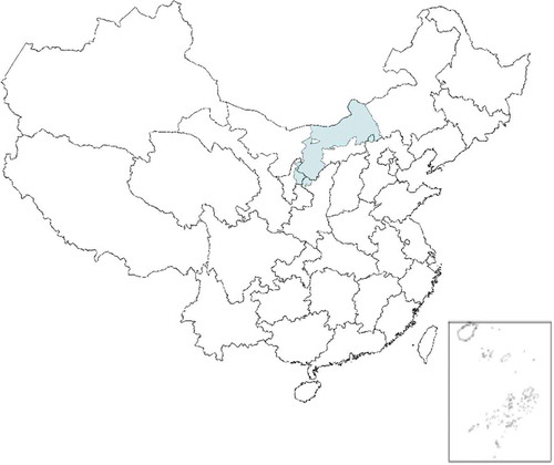
To test the effectiveness of the environmental similarity method, the method was used for predicting the spatial distribution of flea index in a case study. The study area is situated at the epidemic foci of the Mongolian gerbil in the Inner Mongolia Autonomous Region of China is shown in Figure 2. It is located in the region of 37.6°–45° latitude North and 106.5°–114.8° longitude East, mainly distributed in the Wulanchabu, ordos desert steppe and Chahar hills steppe. The elevation within the area ranges from 900 to 3400 m with a total area of approximately 13,8702 km². The annual temperature ranges from 2 to 5°C, and the average annual precipitation is from 200 mm to 360 mm.

Figure 2. Location of study area: the epidemic foci of the Mongolian gerbil.

The surveillance of rodent hosts and fleas was used to calculate the ‘flea index’ as shown in Equation 6(6) $\text{Flea index = }\frac{\text{Number of fleas collected from the rodent hosts examined}}{\text{Number of rodent hosts examined }}$(6) . The number of rodent hosts and fleas from each collection area were used to calculate the flea index, as the risk indicator of plague. Given the characteristics of the environmental conditions and the flea index relationships in this area, climatic, biological, geological, and topographic covariates are the most effective environmental indicators of the spatial variation of plague. Thus, the average annual precipitation, the annual temperature and the annual relative humidity were used to characterize climatic covariates. Biological covariates consist of NDVI and density of rodent host. Topographic and geomorphic covariates include elevation (m), slope gradient (%), aspect, profile curvature, contour curvature, surface area ratio and topographic wetness index (TWI).

(6) $\text{Flea index = }\frac{\text{Number of fleas collected from the rodent hosts examined}}{\text{Number of rodent hosts examined }}$(6)

Climate, vegetation and parent material data were obtained from the Chinese Academy of Sciences Resources and the Environment Scientific Information Centre. Flea index and host density data were provided by Chinese Centre for Disease Control and Prevention. Digital elevation model (DEM) was created from SRTM 90 m resolution terrain data, which was downloaded from the website of Resource and Environment Data Cloud Platforms (http://www.resdc.cn/Default.aspx). Data on slope gradient, aspect, profile curvature and contour curvature were derived from this DEM using ArcGIS software. The surface area ratio was generated with the algorithm proposed by Jenness (2004) and TWI was calculated with the algorithm proposed by Qin et al. (2011). At a given location an environmental vector is formed to characterize the environmental conditions:

(7) $e=\left(e_1,e_2,\dots ,e_m\right)$(7)

where m is the number of environmental covariates used.

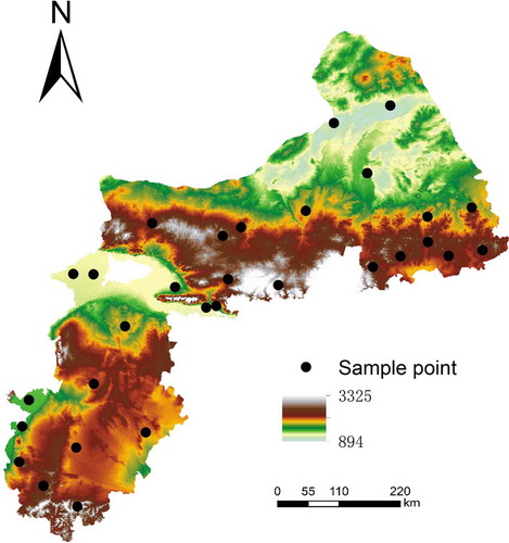
Due to the different resolutions of the environment variables, the final map resolution was set to 1 km. This is because the resolutions of climate and parent material variables are usually at a resolution of 1 km × 1 km grid. Thirty sample points of flea index were collected independently. Figure 3 shows the coverage of the samples in the environmental feature space using elevation as an example.

Figure 3. The location of 30 samples existing in the study area.

4.2. Evaluation and validation

To evaluate and validate the similarity-based approach, a multiple linear regression (MLR) were developed for comparison. To be consistent and comparable, the same climatic, parent material, topographical and biological covariates were used as the predictors and the flea index used as the dependent variable. The 30 samples were used to build the MLR and then the built MLR was used to predict the flea index value at every location across the study area. No uncertainty value was created with this approach.

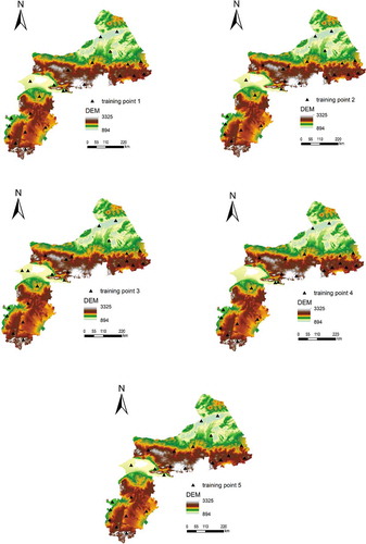
Evaluation and validation was done using repeated subsampling. This is similar to k-fold cross-validation, but we do not use all folds of a split, just one of them each time, as the test set. This gives a good idea of how variable are the evaluation statistics. To take a training sub-sample repeatedly, fit the model with it, and predict at the remaining test points, with so few it’s difficult to decide on a split. The repeated subsampling randomly divided existing samples into training samples and validation samples. The training samples were used prediction mapping, and then the results of the mapping were evaluated by random validation samples. In this study, 30 existing samples was divided into 24 training samples and 6 validation samples 5 times (groups) randomly, Figure 4 show each time of distribution of training samples and validation samples. Two indices, the root mean squared error (RMSE) and mean absolute error (MAE), were used to measured prediction accuracies. The quantified prediction uncertainty was also generated with the environmental similarity method.

Figure 4. Five groups of training samples.

4.3. Results

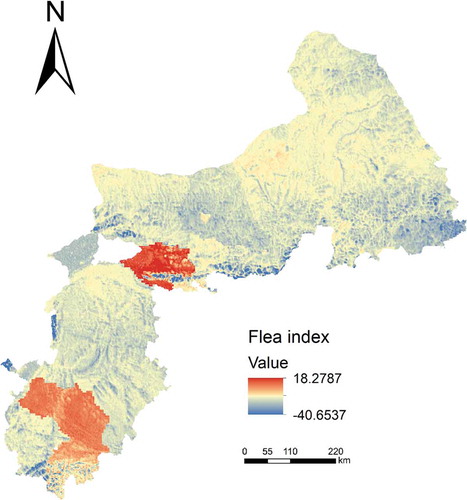
Figure 5 shows the predicted flea index map with the environment similarity method under the limited sample scenario. Under this scenario all samples were used (with uncertainty threshold set to 1.0). The predicted values range from 0 to 12.6577. Comparatively, Figure 6 shows the predicted flea index map with MLR, on which the predicted values range from 18.2787 to −40.6537. The unreasonable predicted negative values were the result of unreasonable extrapolation beyond the information in the available samples. On the flea index maps with the environment similarity method, locations in the northeast part of the study area were assigned relatively low flea index values while the southwest of study area were assigned relatively high flea index values. This spatial distribution pattern matches the actual situation during times of plague epidemic. In contrast, the flea index of the northeast and southwest of study area on the predicted flea index map by MLR was not assigned.

Figure 5. Spatial distribution map of flea index based on environment similarity method.

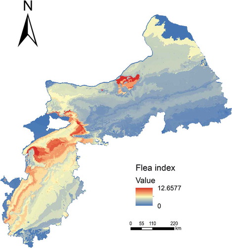
Figure 6. Spatial distribution map of flea index based on MLR.

Figure 7 shows the prediction uncertainty produced with the environment similarity method. The flea index samples are mainly located in the area where prediction uncertainty is generally low and can represent those areas well. In contrast, high prediction uncertainty values were assigned to the northeast of study area, where the environmental conditions are very different from what are captured by the existing samples.

Figure 7. Uncertainty distribution map.

The prediction accuracies from the validation samples are shown in Table 1. The RMSE and MAE of the similarity-based method are 6.6493 and 1.2713, respectively, and are lower than those of the MLR. This shows that for the same number of samples the similarity-based method has a higher accuracy.

Table 1. Prediction accuracy of environmental similarity and MLR methods.

Method	RMSE	MAE
Environmental similarity	6.6493	1.2713
MLR	7.293	2.928

5. Discussion

The similarity-based method is based on the Third Law of Geography and is different from the spatial prediction methods based on other principles such as the First Law of Geography or the statistical theories. The similarity-based method focuses on the comparison of a sample point and a prediction point rather than based on explicit relationships derived from full set of samples. This allow the prediction method to capture spatial variation at much detailed level, which might be important for prediction of plague risk.

clearly, the selection of environmental covariates plays a critical role in the quality of prediction based on the similarity method. The selected environmental covariates need to reflect the factors which impact the distribution of flea which carry the virus for the plague. In this study variables on climate, vegetation, topography and soils were used as environmental covariates. Needless to say that this set of variables is not comprehensive enough to characterize the environmental habitats of the flea. Spatial connectivity would also play an important role in spatial variation of plague risk. This variable was not included in this study.

The use of comparison of geographic configurations with the similarity method, rather than the explicit extraction of relationships, allows uncertainty associated with the prediction be quantified. This uncertainty could be used to further assess the spatial distribution of the prediction accuracy and assist in allocation of additional sampling efforts.

6. Conclusions

This paper presents a method based on environmental similarity for predicting spatial variation of risk in terms of flea index. This method is suitable for situations where only a limited numbers of plague field data (such as flea index) available. The method also allows for the quantification of prediction uncertainty at unvisited locations. With the assistance of the prediction uncertainty measure, further field sampling efforts can be effectively allocated and sampling resources can be used wisely by sampling the under-represented areas with greater precedence. The method has the potential to provide better assistance in predicting the spatial distribution of plague outbreaks.

Acknowledgements

The work reported here was supported by grants from the National Natural Science Foundation of China (Project No.: 41871300, 41431177, 41601413), PAPD, and the Outstanding Innovation Team in Colleges and Universities in Jiangsu Province. A-Xing Zhu received further support through the Vilas Associate Award, the Hammel Faculty Fellow Award, the Manasse Chair Professorship from the University of Wisconsin-Madison, which are greatly appreciated.

Disclosure statement

No potential conflict of interest was reported by the authors.

Additional information

Funding

This work was supported by the National Natural Science Foundation of China [41431177, 41601413].

References

- Bihrmann, K., S. S. Nielsen, N. Toft, and A. K. Ersbøll. 2012. “Spatial Differences in Occurrence of Paratuberculosis in Danish Dairy Herds and in Control Programme participation.” Preventive Veterinary Medicine 103 (2–3): 112–119. doi:10.1016/j.prevetmed.2011.09.015.
- Buckley, Y. M. 2015. “Generalised linear models”. Journal of the Royal Statistical Society 135 (3): 370–384. doi:doi:10.1093/acprof:oso/9780199672547.003.0007
- Fang, X. Y., R. F. Yang, Q. Y. Liu, X. Q. Dong, and X. U. Lei. 2012. “A Novel Method for Typing Natural Plague Foci in China II. Research on the Typing Methods for Natural Plague Foci.” Zhonghua Liu Xing Bing Xue Za Zhi 33 (2): 234–238.
- Gage, K. L., T. R. Burkot, R. J. Eisen, and E. B. Hayes. 2008. “Climate and Vectorborne Diseases.” American Journal of Preventive Medicine 35 (5): 0–450. doi:10.1016/j.amepre.2008.08.030.
- Goovaerts, P. 1999. “Geostatistics in Soil Science: State-of-the-art and perspectives.” Geoderma 89 (1–2): 1–45. doi:10.1016/S0016-7061(98)00078-0.
- Hengl, T., G. B. M. Heuvelink, B. Kempen, J. G. B. Leenaars, M. G. Walsh, K. D. Shepherd, A. Sila, R. A. MacMillan, J. Mendes de Jesus, L. Tamene, et al. 2015. “Mapping Soil Properties of Africa at 250 M Resolution: Random Forests Significantly Improve Current Predictions.” Plos One 10 (6): e0125814. doi:10.1371/journal.pone.0125814.
- Hu, W., A. Clements, G. Williams, and S. Tong. 2011. “Spatial Analysis of Notified Dengue Fever infections.” Epidemiology and Infection 139 (3): 391–399. doi:10.1017/S0950268810000713.
- Isaaks, E. H., and M. R. Srivastava. 1989. “Applied geostatistics.”
- Jenness, J. S. 2004. “Calculating Landscape Surface Area from Digital Elevation models.” Wildlife Society Bulletin 32 (3): 829–839. doi:10.2193/0091-7648(2004)032[0829:CLSAFD]2.0.CO;2.
- Krige, D. G. 1951. “A Statistical Approach to Some Basic Mine Valuation Problems on the Witwatersrand.” Journal of the Chemical, Metallurgical and Mining Society of South Africa 52 (6): 119–139.
- Lin, L., and G. Zi-Hou. 2014. “Relation between Natural Environmental Factors and plague.” Chinese Journal of Control of Endemic Diseases 29 (3): 177 179.
- Parmenter, R. R., E. P. Yadav, C. A. Parmenter, P. Ettestad, and K. L. Gage. 1999. “Incidence of Plague Associated with Increased Winter-spring Precipitation in New Mexico.” The American Journal of Tropical Medicine and Hygiene 61 (5): 814–821. doi:10.4269/ajtmh.1999.61.814.
- Qin, C.-Z., A.-X. Zhu, T. Pei, B.-L. Li, T. Scholten, T. Behrens, and C.-H. Zhou. 2011. “An Approach to Computing Topographic Wetness Index Based on Maximum Downslope gradient.” Precision Agriculture 12 (1): 32–43. doi:10.1007/s11119-009-9152-y.
- Shi, X., A.-X. Zhu, J. E. Burt, F. Qi, and D. Simonson. 2004. “A Case-based Reasoning Approach to Fuzzy Soil mapping.” Soil Science Society of America Journal 68 (3): 885–894. doi:10.2136/sssaj2004.8850.
- Singchai, C., V. Deesin, R. Srisawat, S. Yamput, T. Phanphuwong, P. Pongwatanakulsiri, E. Vimutisunthorn, and P. Puthavathana. 2003. “Surveillance of Commensal Rat and Shrew Populations in the Bangkok Area with References to Flea Index as the Risk Indicator of plague.” Journal of the Medical Association of Thailand = Chotmaihet Thangphaet 86 (9): 795.
- Stenseth, N. C., B. B. Atshabar, M. Begon, S. R. Belmain, E. Bertherat, E. Carniel, K. L. Gage, H. Leirs, and L. Rahalison. 2008. “Plague: Past, Present, and Future.” PLoS Medicine 5 (1): 9–13. doi:10.1371/journal.pmed.0050003.
- van der Ploeg, R. R., W. Böhm, and M. B. Kirkham. 1999. “On the Origin of the Theory of Mineral Nutrition of Plants and the Law of the minimum.” Soil Science Society of America Journal 63 (5): 1055–1062. doi:10.2136/sssaj1999.6351055x.
- World Health Organization (WHO). 2017. “Plague - Madagascar.” https://www.who.int/csr/don/27-november-2017-plague-madagascar/en/
- Xu, L., Q. Liu, L. C. Stige, T. Ben Ari, X. Fang, K.-S. Chan, S. Wang, N. C. Stenseth, and Z. Zhang. 2011. “Nonlinear Effect of Climate on Plague during the Third Pandemic in China.” Proceedings of the National Academy of Sciences of the United States of America 108 (25): 10214–10219. doi:10.1073/pnas.1019486108.
- Zhang, A. P., R. J. Wei, H. M. Xiong, and Z. Y. Wang. 2016. “Advance to the Research of the Climate Factor Effect on the Distribution of plague.” Zhonghua Yu Fang Yi Xue Za Zhi 50 (5): 459–462. doi:10.3760/cma.j..0253-9624.2016.05.015.
- Zhao, Q. F., and J. X. Yin. 2016. “Analysis for the Compositions of Plague Natural Foci and Their Roles.” Modern Preventive Medicine 43 (2): 370-372.
- Zhu, A. X., J. Liu, F. Du, S. J. Zhang, C. Z. Qin, J. Burt, and T. Scholten. 2015. “Predictive Soil Mapping with LimitedSample Data.” European Journal of Soil Science 66 (3): 535–547. doi: 10.1111/ejss.12244.
- Zhu, A.-X., G. Lu, J. Liu, C.-Z. Qin, and C. Zhou. 2018. “Spatial Prediction Based on Third Law of Geography.” Annals of GIS 24 (4): 225–240. doi:10.1080/19475683.2018.1534890.
- Zhu, A.-X., L. Band, R. Vertessy, and B. Dutton. 1997. “Derivation of Soil Properties Using a Soil Land Inference Model (Solim).” Soil Science Society of America Journal 61 (2): 523. doi:10.2136/sssaj1997.03615995006100020022x.
- Zhuang, D., H. Du, Y. Wang, X. Jiang, X. Shi, and D. Yan. 2016. “Probing the Spatial Cluster of Meriones Unguiculatus Using the Nest Flea Index Based on GIS technology”. Acta Tropica 163: 157–166. doi:10.1016/j.actatropica.2016.08.007.