A web-based spatial decision support system for monitoring the risk of water contamination in private wells

ABSTRACT

Long-term exposure to contaminated water can cause health effects, such as cancer. Accurate spatial prediction of inorganic compounds (e.g. arsenic) and pathogens in groundwater is critical for water supply management. Ideally, environmental health agencies would have access to an early warning system to alert well owners of risks of such contamination. The estimation and dissemination of these risks can be facilitated by the combination of Geographic Information Systems and spatial analysis capabilities – i.e., spatial decision support system (SDSS). However, the use of SDSS, especially web-based SDSS, is rare for spatially explicit studies of drinking water quality of private wells. In this study, we introduce the interactive Well Water Risk Estimation(iWWRE), a web-based SDSS to facilitate the monitoring of water contamination in private wells across Gaston County, North Carolina (US). Our system implements geoprocessing web services and generates dynamic spatial analysis results based on a database of private wells. Environmental health scientists using our system can conduct fine-grained spatial interpolation on 1) a particular type of contaminant such as arsenic, 2) on various subsets through a temporal query. Visuals consist of an estimation map, cross validation information, Kriging variance and contour lines that delineate areas with maximum contaminant levels (MCL), as set by the US Environmental Protection Agency (EPA). Our web-based SDSS was developed jointly with environmental health specialists who found it particularly critical for the monitoring of local contamination trends, and a useful tool to reach out to private well users in highly elevated contaminated areas.

KEYWORDS:

• Geoprocessing services
• health
• interpolation
• private well
• risk
• spatial decision support system
• water contamination

1. Introduction

Although the quality of drinking water in the United States (US) is considered to be one of the best in the world (Global Open Data Index 2016), waterborne diseases remain a concern in some regions (Whitacre 2009). According to the US Environmental Protection Agency (EPA), approximately 13 million households (45 million Americans) rely on unregulated private wells for drinking water (Strauss et al. 2001; U.S. EPA 2019), and private wells are generally more vulnerable than municipal water for exposure to various contaminants. Long-term exposure to contaminated water can cause health effects, for instance gastrointestinal illnesses, damage to the nervous system, liver complications and chronic diseases such as cancer. The severity of health impacts is also influenced by other factors, such as the type and concentration of contaminants in the water, the quantity of water consumed and the duration of exposure.

Several studies that have attempted to estimate the risk of drinking water contamination, see for instance Rahman (2002); Shrestha et al. (2003); Maharjan et al. (2005); Liu, Ming, and Ankumah (2005); Murray, Uber, and Janke (2006); Buschmann et al. (2008); Rogan and Brady (2009); Wongsasuluk et al. (2014). For example, Rahman (2002) studied the association between arsenic and geology, and its health effects, while Murray, Uber, and Janke (2006) introduced a model for estimating both spatial and temporal distribution of health effects related to contaminated drinking water.

Therefore, a system to monitor groundwater water quality is crucial for environmental health specialists as they need to make decisions in a timely manner, in an effort to alert residents of the risks posed by contaminated groundwater and conduct additional sampling in areas deemed at risk (Delmelle and Goovaerts 2009; Rogerson et al. 2004).

These decisions can be facilitated by using a decision support system (DSS), which is an interactive computer-based system that provides information and analysis to support the identification of solutions for complex problems. A spatial decision support systems (SDSS) is a special kind of decision system that combines spatial data processing capabilities from geographic information systems (GIS) with spatial analysis and modelling (Sugumaran and Degroote 2010; Malczewski 1999; Densham 1991; Delmelle et al. 2011). A SDSS includes two components: spatial and decision support. The spatial component serves to manage, analyse and display spatially referenced data, while the decision support element allows decision makers to use spatial statistical functions to achieve sound decisions addressing spatially complex issues (Ghosh 2008).

However, only a few studies at the intersection of groundwater quality and public health incorporate SDSS in which GIS has maintained a pivotal role. For example, GIS has been used to map arsenic distribution (Gaus et al. 2003; Samadder and Subbarao 2007; Kim et al. 2011; Dummer et al. 2015) and groundwater vulnerability (Nobre et al. 2007), while some other studies have compared geostatistical approaches to estimate contamination concentration (Goovaerts et al. 2005; Meliker et al. 2008).

More recently, GIS has been used to design groundwater quality monitoring networks (Preziosi, Petrangeli, and Giuliano 2013; Esquivel, Morales, and Esteller 2015). It is generally acknowledged that spatial interpolation is the process to estimate the spatial variation of groundwater by using known observations of groundwater quality to predict at locations where no samples have been collected (see for instance Goovaerts 1997). For instance, Nas and Berktay (2010) used GIS and ordinary Kriging to generate groundwater quality map, and applied Monte Carlo simulations to estimate exposure to arsenic in drinking water at the individual level, and more recently geostatistical methods were developed for accurate estimation of municipal water contamination in Flint, Michigan (Goovaerts 2017; Hanna-Attisha et al. 2016). Temporally explicit contamination maps may be critical to understand the change in the spatial extent of contamination, and whether efforts to reduce contamination are effective.

1.1. Geoprocessing web services

The advancement of web and Internet technologies has stimulated the development and use of SDSS over the web (Sugumaran and Degroote 2010). A series of studies have developed SDSS combined with web-based GIS capabilities in different domains, such as natural resource management (Choi, Engel, and Farnsworth 2005; Sugumaran, Meyer, and Davis 2004; Tang et al. 2017; Zeng et al. 2012), earth science (Mwaura and Kada 2017; Zhang, Zhao, and Weidong 2010), business location (Jung and Sun 2006), and health (Kelly et al. 2011; Delmelle et al. 2011; Kienberger et al. 2013; Delmelle et al. 2014). Geoprocessing services play a key role in these web-based SDSS applications. The development and use of geoprocessing services fall within the domain of service-oriented computing and cloud computing, substantially driven by state-of-the-art cyberinfrastructure-enabled GIS (aka CyberGIS) or spatial cyberinfrastructure (see Wang 2010; Yang et al. 2010).

Specifically, geoprocessing services have the ability to process geospatial data and generate results over Internet (Peng and Tsou 2003; Fu and Sun 2010), which enhance the capabilities of Web GIS (conventional Web GIS focus on data- or map-based services). A single spatial data processing or spatial analysis capability can be encapsulated into an individual geoprocessing service. A set of geoprocessing capabilities can be connected and published into a geoprocessing service to provide complicated spatial analytical functionalities. As the resolution of a spatial problem typically involves multiple spatial data processing and spatial analyses, multiple geoprocessing steps are often chained through scientific workflow technologies as an important cyberinfrastructure capability (see Wang 2010; Tang et al. 2017).

The use of geoprocessing services has been stimulated by the development of Web Processing Service (WPS), which is an interoperable geoprocessing service standard by Open Geospatial Consortium (OGC). Geoprocessing services have been applied in various domains for spatial decision support and, as a result, a series of web-based SDSS have been developed(e.g., Burdziej 2012; Li et al. 2013; Lin et al. 2015; Modica et al. 2016; Mwaura and Kada 2017; Tang et al. 2017; Zhang et al. 2019). Although the application of web-based SDSS with support from geoprocessing services is relatively common for air quality, weather and environmental data -such as the INTAMAP project (Distefano et al. 2015; Hiemstra et al. 2009; Pebesma et al. 2011; Schäjfler et al. 2010; Williams et al. 2011), it is relatively rare into the study of groundwater quality, particularly, private wells. This greatly limits the processing and analysis of relevant geospatial data to inform timely decision makers for potential public health issues caused by groundwater quality.

As underlined by Hoover et al. (2014), most states across the US have used flyers, television advertisements and focus groups to disseminate information on water quality and health impact of continued exposure to contaminated water. Several states have developed static maps of groundwater levels and water conditions. The United States Geological Survey (USGS) has developed StreamStats, a web based application that provides critical information such as basin delineations, basin-characteristic measurements, and estimates of streamflow statistics, which can then be used by engineers, managers, and planners to make informed decisions on water-related activities (Ries et al. 2008), however such systems do not provide continuous information on groundwater contamination from private wells. Some states have sought to use test results to produce interactive maps of well water quality for common contaminants (e.g. Minnesota,¹ New Jersey,² Oregon,³ and Wisconsin⁴ to cite a few). Along the same vein, a few scholars have developed GIS systems to visualize the variation of and water quality (Choi, Engel, and Farnsworth 2005; Dymond et al. 2004; Jankowski, Tsou, and Wright 2007). These interactive maps provide limited, aggregated information to the general public, and are limited in geoprocessing capabilities. A notable exception is the paper by Hoover et al. (2014), which attempts to apply web GIS in the study of groundwater quality. However, most of the functionalities developed in Hoover et al. (2014) focused on web-based mapping/visualization instead of geoprocessing services (web-based geoprocessing).

In North Carolina, there is no system in place to provide (near) real-time information and geospatial analytics support to private well owners on the quality of the groundwater they rely on, reducing their awareness of the risk posed by contaminated water. Needed are systems that 1) use well data to provide timely information and contamination risks to both individuals and health officials to support decision-making, and 2) educate well users as to the best practices to manage their water. To fill this gap, in this study, we develop a web-based SDSS with support from geoprocessing services driven by scientific workflows to monitor the risk of water contamination in private wells across Gaston County, North Carolina (USA). This web-based SDSS allows decision makers, environmental health specialists, or the public to perform automated spatial data processing and analyse data on demand. Users can choose the type of inorganic contamination to be mapped, 2) conduct temporal queries and 3) set parameters of the spatial analysis methods. Ultimately, our system provides contamination estimation results in the form of maps and contours reflecting maximum contaminant levels for drinking water from the US EPA.

The rest of the article is organized as follows. In Section 2, the study area and data are introduced. The implementation of our web-based SDSS system is described in Section 3, while an example using arsenic data is presented in Section 4. In Section 5, we discuss (1) scalability of our approach based on computational experiment and (2) the practicality of our system, where we evaluate our system with a local environmental specialist, and suggest avenues for future research.

2. Study area and data

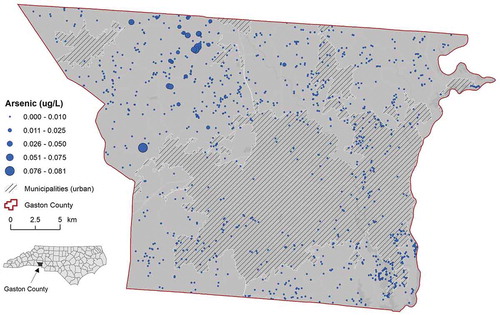
Our study area is located in Gaston County (North Carolina, US). According to the 2018 US Census Bureau, the population in Gaston County was 222,846 with 15.1% living in poverty. In 2015, the Gaston County Department of Health and Human Services was awarded ‘Heathy Wells’, a five-year grant from the Centres for Disease Control and Prevention (CDC) to establish an exhaustive spatial database of the County’s wells through conversion of paper records dating back to 1989. The Private Well data layer, built in a GIS, describes wells that have been installed, repaired, and abandoned since 1989. Approximately n = 8,500 paper-based well permits were digitized and historical samples (2011–2018) on inorganic contaminants was linked to n = 1,235 geocoded wells (Owusu et al. 2017). However, 152 observations were repeat samples (water tested multiple times throughout the study area⁵), and hence we opted to retain the first observation, resulting in a set of n = 1,083 observations. Inorganic data for private wells were obtained from the Gaston County Department of Health and Human Services (GC-DHHS) for 2011 through 2017. Each observation is characterized by geographic coordinates, a date when water was analysed and concentration levels for various inorganic compounds. Figure 1 shows the spatial distribution of private wells in our study region, where graduate symbology reflects observed arsenic levels. We obtained information on various inorganic contaminants such as arsenic, chromium, copper, fluoride, lead, mercury, nitrate, nitrite among other from Gaston County Department of Health and Human Services.

Figure 1. Map of private wells with contamination information in Gaston County, NC (2011–2017).

3. Methodology

In this section, we present the system architecture, scientific workflow of the WPS model, and the interface of our web-based SDSS as interactive Well Water Risk Estimation (iWWRE). The ultimate objective of iWWRE is to address the need of environmental specialists to produce and interactive estimation map of the risk of water contamination reported from private wells.

3.1. System architecture

Following Armstrong, Densham, and Rushton (1986), we develop a web-based SDSS framework with four modules: database management, modelbase management, display and report generators, and user interface along with a new module, web services (Figure 2).

Figure 2. Conceptual architecture of the web-based SDSS framework for monitoring the risk of water contamination in private wells.

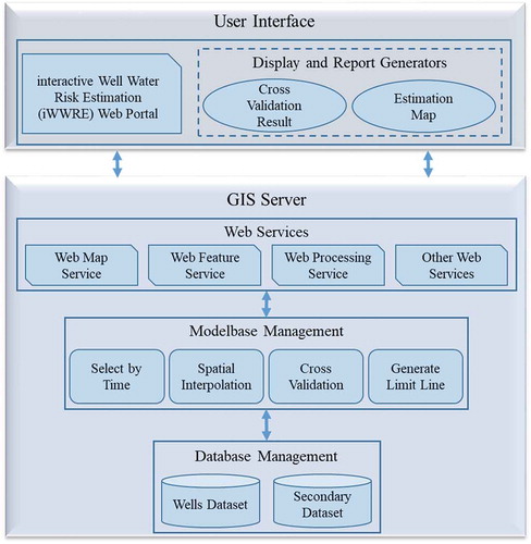
We resort to an application and a GIS server. ESRI ArcGIS Server 10.6 is adopted to provide web services including Web Map Service (WMS), Web Feature Service (WFS) and WPS, while in the GIS server, two SDSS modules, database management and modelbase management, are equipped to manage dataset and conduct analysis.

We use two sets of spatial data in this system: wells data and secondary data. Wells data contain geographic coordinates and contamination information, while secondary data consist of geology and township layers. The modelbase management module provides several GIS algorithms and spatial analysis approaches to support the generation of an estimation map of water contamination measured at private wells. These GIS algorithms and spatial analysis approaches include 1) selection of wells by time range, 2) spatial interpolation, 3) uncertainty from the spatial interpolation, and 4) generation of contour lines around area characterized by high-risk contamination. The temporal query capability of our system is motivated by the fact that the quality of the groundwater can change over time – in the case of arsenic which appears to be naturally occurring, conducting spatial interpolation on different temporal subsets may not provide as much evidence of a change, as it could be the case with other inorganic compounds such as nitrate that may reflect seasonal agricultural practices. Importantly, we justify this functionality by the need of environmental health specialists to learn whether remediation procedures (reverse osmosis, well chlorination) may have had an impact on the reduction of the contaminants over time.

Both data and spatial analysis algorithms are published via a web GIS server as web services. The interface of iWWRE, as in the module of display and report generators, is developed using HTML, JavaScript, and ArcGIS application programming interface (API) 3.30. The interpolated maps, cross validation results and uncertainty results are visualized in the interface after running the geoprocessing service.

3.2. A scientific workflow of geoprocessing services

The scientific workflow used in this article is summarized in Figure 3. Because of their temporal information, observations on water contaminations can be queried using a SQL-formatted criterion based on a given time period, and spatial interpolation is then implemented on the selected set. In this article, we implement both Inverse Distance Weighting (IDW) and Kriging as interpolation approaches. It is generally recognized that Kriging yields a more accurate interpolation surface minimizing the variance of prediction error – or Kriging variance (Goovaerts 1997), but at the cost of a more thorough variogram analysis, a procedure that can be challenging for users with limited GIS or spatial statistics background. IDW on the other hand does not use spatial autocorrelation information to guide the interpolation process (Lam 1983). Prior studies have shown that both approaches have advantages, generally depending on the strength of the covariance structure summarizing covariates (such as well depth) among nearby observations and the geographic distribution of the wells (Gong, Mattevada, and O’Bryant 2014). Due to the smoothing effect⁶ of Kriging that leads to overestimate minima than underestimate maxima (Olea and Pawlowsky 1996; Yamamoto 2005), IDW can perform better in predicting high-risk regions, while Kriging may be better in predicting low-risk areas (Mirzaei and Sakizadeh 2016). Alternatively, the surface of regions deemed at risk may be overestimated by one interpolation approaches over another (Elumalai et al. 2017). In iWWRE, the user has the choice of the interpolation approaches.

Figure 3. The scientific workflow of WPS model for monitoring the risk of water contamination in private wells. (The function ‘Extract by Boundary’ clips resulting raster data to the boundary of the study area.).

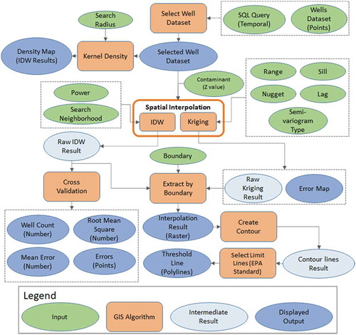
When IDW is selected for the interpolation approach, the user can decide on the choice of power coefficient and search neighbourhood. The power coefficient is the exponent of distance that essentially controls the contribution of surrounding points to the interpolated value. For example, a larger power means that nearest points will contribute more to the value that is interpolated, resulting in a more ‘choppy’ raster. Search neighbourhood determines which surrounding points will be used to control the output. Four options are made available to the user: standard, smooth, standard circular, and smooth circular. The standard approach uses an ellipse as the searching neighbourhood, while the smooth approach contains both an outer and an inner ellipse. The selection of search neighbourhoods is influenced by the input data and the interpolation result based on users’ judgement. For isotropic processes, the shape of the search neighbourhood should be a circle; in contrast, in the presence of anisotropy dictated for instance by geological formations, an elliptical search may be preferred. Smooth and smooth circular create an outer ellipse/circular and an inner ellipse/circular, and all the points within these three ellipses/circulars are used in the interpolation. By doing so, smooth and smooth circular can generate smoother interpolation results than standard approaches.

In Kriging, interpolation results can be obtained using default variogram parameters, while users with advanced geostatistical knowledge can set parameters for the variogram, including the range (where the variogram flattens out), nugget, sill, lag, and variogram type. iWWRE uses Ordinary Kriging (OK) as the geostatistical model (in OK the mean is unknown but constant, and is estimated as part of the solution of the interpolation equations). The user can choose among five variogram types: spherical (default), circular, exponential, gaussian, and linear.

In addition to the interpolated surface, we generate contour lines based on the maximum contaminant level (MCL) for drinking water quality from EPA. This information is particularly useful for environmental health decision makers if they need to make decision on additional sampling.

3.3. Uncertainty

In Kriging, the uncertainty is estimated by the Kriging variance, which is a function of the covariance structure -as defined by the variogram and the spatial distribution of observations (Delmelle and Goovaerts 2009). However, IDW does not yield a prediction error surface and instead we report cross validation results reflecting the uncertainty of the IDW approaches. Following the approach set out by Tomczak (1998), we use a leave-one-out cross validation (also known as jackknife) to calculate the uncertainty of the IDW approach at each point. The cross validation approach returns the root mean square error (RMSE, Equation (1)(1) $RMSE=\sqrt{\frac{1}{n}\sum _{i=1}^n{\left({\hat{z}}_i-z_i\right)}^2}$(1) ), mean error (ME, Equation (2)(2) $ME=\frac{1}{n}\sum _{i=1}^n\left({\hat{z}}_i-z_i\right)$(2) ) at each point (well); and they are stored as a point feature layer (Gong, Mattevada, and O’Bryant 2014).

(1) $RMSE=\sqrt{\frac{1}{n}\sum _{i=1}^n{\left({\hat{z}}_i-z_i\right)}^2}$(1)

(2) $ME=\frac{1}{n}\sum _{i=1}^n\left({\hat{z}}_i-z_i\right)$(2)

where ${\hat{z}}_i$ and $z_i$ are the estimated and observed contamination value of the i^th data, and n is the number of selected observations (wells). The user can choose to display the results of the cross-validation statistic; in the case of the mean error, the point feature layer is coloured following a diverging scheme.

Because IDW does not provide a continuous map of uncertainty, we implemented the Kernel Density Estimation (KDE) algorithm, which essentially reflects the spatial distribution of selected wells and is used as a proxy for confidence. Regions with high KDE values can be considered as regions with more collections of well contaminants information. Used in concert with threshold lines, KDE values can address one facet of uncertainty where individuals living in frequently tested area (high KDE) would have a higher ‘confidence’ in the interpolated map.

3.4. Interface

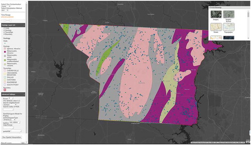
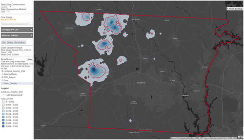
The interface of iWWRE (Figure 4) allows users to specify parameters, apply functionality and visualize results in an interactive manner. First, users choose an inorganic contamination (e.g. arsenic), spanning over a specific time range.⁷ These two parameters (variable and time range) are required for the spatial interpolation process. Second, the users must select whether to conduct the IDW or the Kriging interpolation, and set customized parameters (e.g., power coefficients, search neighbourhood for IDW; range, sill, nugget for Kriging model) or decide on default parameters. Third, once the geoprocessing scientific workflow is executed, the cross-validation statistics for IDW -including the count of selected wells, RMSE, and ME- are computed. Fourth, selected wells, interpolation surface and ‘limit lines’ corresponding to the EPA MCL are displayed. If the IDW method is selected, cross-validation results and a KDE map are also provided. When Ordinary Kriging is chosen, the variance of prediction error (Kriging variance) is also provided. All published WMS, WFS, and results of WPS are shown in the map interface. In addition to basic functionality of a web map such as zoom and pan, the map interface allows the user to query the information of reference layers. Finally, secondary information (geology, townships, and boundary layers) can be turned on and off.

Figure 4. The interface of iWWR.

4. Case study

We illustrate the merits of the iWWRE using a private wells dataset in Gaston County, North Carolina (US) and arsenic as the inorganic contaminant from 2011 to 2017. Figures 1 and 4 show the spatial distribution of the private wells overlaid with layers of wells, geology and townships. We performed spatial interpolation, both IDW and Kriging, on the entire well dataset, and using yearly well data. An example of the interpolation spanning the entire period is given in Figure 5, with areas in the western region experiencing higher levels of arsenic (dark blue). The lowest values for arsenic were made transparent so the end user could focus on regions experiencing elevated values. We used the EPA MCL of 0.01 mg/l to delineate areas where additional sampling is ‘Highly Recommended’.

Figure 5. An example of IDW interpolation applied to arsenic, 2011–2017.

4.1. KDE with default and user-defined parameters

Figure 6 illustrates KDE maps using the default bandwidth (from ArcGIS default bandwidth algorithm) and user-defined bandwidth (the latter are also reproduced in Figure 7). User defined bandwidths corresponds to the average distance to the ten closest neighbours,⁸ a choice motivated by the minimum number of 10 neighbours for IDW. Dark blue coloured regions denote high KDE values, while brown regions are indicative of low density of private wells. The default bandwidth is much larger than user-defined bandwidth. For instance, user-defined bandwidths (average of the 10 closest neighbours) range from 3,295 to 4,565 metres depending on the spatial distribution of wells for each year, while the default bandwidths are between 11,631 and 12,551meters. KDE estimated with default bandwidths tend to oversmooth the spatial distribution of the wells and are not useful when coupled with IDW interpolated maps.

Figure 6. Comparison of density maps between default bandwidth (top) and customized bandwidth (bottom) for kernel density from 2011 to 2017.

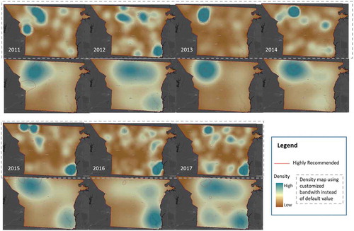
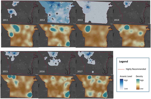
Figure 7. Arsenic interpolation by means of IDW and KDE maps for wells from 2011 to 2017.

4.2. IDW and KDE

Using IDW and KDE results together can provide valuable information to interpret our results and identify areas deemed in risk of water contamination. Figure 7 summarized arsenic interpolation and KDE maps with user-defined bandwidths. In 2011, two areas (with smooth boundaries in the northwestern corner of the county) were identified as high risk for arsenic contamination, and these two areas were characterized by high, localized KDE values, giving us greater confidence in the interpolation result. For 2016, only a relatively small area exhibited high arsenic concentration, while the KDE map suggested that there were too few samples in that region to garner enough confidence in our interpolation.

Table 1 reports cross-validation results for all time ranges. In general, RMSE decreases with increasing number of wells (2016 exhibits lowest of the yearly RMSE as the number of wells (count) is the highest among those seven years). However, the number of wells is not the only factor that affects RMSE, but the quality of the interpolation (an overall RMSE value close to zero suggests an interpolation that better honours input observations).

Table 1. Summary of cross validation results for arsenic in different time ranges (count: number of wells).

Year	Root Mean Square (ug/L)	Count	Mean Error (ug/L)
2011	0.0087	152	−0.0004
2012	0.0022	154	−0.0001
2013	0.0033	128	0.0006
2014	0.0057	143	0.0003
2015	0.0048	151	0.0001
2016	0.0014	211	−0.000004
2017	0.0023	185	0.0001
2011–2017	0.0044	1083	0.00004

4.3. Kriging

We also generated Ordinary Kriging results (interpolation and Kriging variance) using user-defined variogram parameters⁹ (‘OK’) and compared those to default values for OK (‘default OK’)- as estimated automatically by the ESRI software, in Figures 8 and 9, respectively. In the Kriging variance maps, brown coloured areas denote high Kriging variance.

Figure 8. Interpolation and error maps for OK from 2011 to 2017, with user-defined parameters.

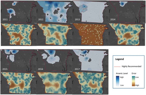
Figure 9. Interpolation and density maps for OK with default parameters from 2011 to 2017.

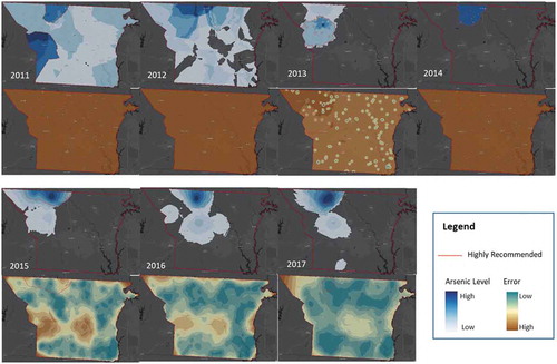
If the user is able to conduct an empirical variogram analysis and identify appropriate parameters, the resulting interpolation surface will better reflect the covariance structure of the variable under study and lead to a more accurate interpolation (Figure 8). The high Kriging variance of 2013 suggests that the end-user should be very cautious when using the interpolated map. In Figure 9, the Kriging variance maps for ‘default OK’ for the years 2011, 2012 and 2014 are not informative – although ESRI does not publish its algorithm to estimate variogram parameters-, it is evident from the ‘default OK’ error maps that the range is extremely small, leading to a very high error throughout the area under study. In other words, the interpolation results using user-defined parameters (‘OK’) provides more suitable results.

4.4. IDW versus OK

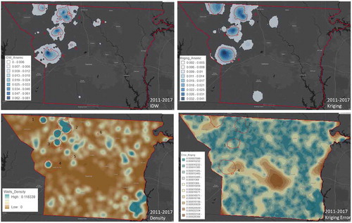
Using all arsenic results from 2001–2017, we now compare the results of IDW and OK, along with KDE and Kriging variance maps for the all the wells from 2011 to 2017. From Figure 10, both interpolation methods provided relatively similar results (correlation = 0.894). We identified four distinct ‘clusters’¹⁰ above the MCL lines in the northwestern section of the county, while IDW identified two more. The threshold contour lines generated from the OK interpolation maps appear less smooth than the ones from IDW. The Kriging variance map shows that site 2 and 3 have lower errors than those in site 1 and 4, but when using KDE as the indicator of confidence, it appears that all these four clusters exhibit every high KDE values. Two additional, smaller clusters (at sites 5 and 6) were extracted from IDW, but both maps of IDW and OK produces relatively similar arsenic values for those two regions. Mirzaei and Sakizadeh (2016) claimed that IDW can perform better in predicting high-risk areas, and our results uphold their finding. Although the KDE does not result in a prediction error value, its spatial pattern visually coincide with the one of the Kriging variance (correlation: −0.527), and may thus provide an alternative to address the absence of uncertainty information when relying on IDW.

Figure 10. Comparison of interpolation results for IDW and OK from 2011 to 2017.

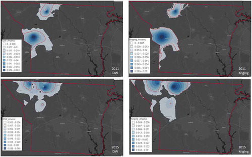
We also compared results of estimation maps of IDW and OK in 2011 and 2015 (Figure 11), and the results exhibited strong similarities. Therefore, users with limited knowledge of geostatistics can use IDW to generate interpolation results, with the assistance of a density map for interpretation. While users with advanced knowledge of OK can use their own values for the variogram model to generate interpolation results as well as error maps.

Figure 11. Comparison of risk estimation maps for IDW and OK in 2011 and 2015.

5. Discussion and evaluation

Our web-based SDSS generates dynamic and interactive maps of groundwater contaminants, and can overlay secondary data with the ultimate goal to monitor in (near) real-time, the risk of water contamination in private wells. This spatially explicit analytics platform needs to inform environmental health specialists who need to make timely decision to, for example, 1) alert residents on the potential risks from contaminated groundwater, and 2) conduct more samples to confirm. This system is applied to inorganic contaminants linked to private wells in Gaston County in North Carolina. The IDW algorithm yielded results comparable to Kriging, but was lacking an uncertainty metric. Hence, we suggested combining both cross-validation and kernel density estimation, the latter reflecting the density of wells; together CV and KDE can ultimately shed light on the confidence of the interpolation results. For users with limited geostatistical background, this approach (IDW+CV+KDE) could provide an alternative option. Although the IDW approach can be implemented for the general public, we recommend environmental health specialists relying on Kriging-based approaches that use variogram models and provide directly prediction error.

In this study, we present a novel solution of generating dynamic results: a web-based SDSS implementing geoprocessing web service of a scientific workflow for the spatial interpolation model. Several studies in web-based SDSS employ WPS to generated dynamic results (Yao et al. 2017), and some of them allow users to set or select parameters of WPS (Mwaura and Kada 2017). However, few studies have investigated the advantages of utilizing geoprocessing services to the study of groundwater quality particularly, private wells. The geoprocessing services driven by scientific workflow has the advantage of organizing complicated spatial analysis into modules in a visually intuitive interface without the requirement of programming skills (Best et al. 2007). Publishing geoprocessing services as WPS offers the capability of parameter settings to the end-user, which expand the feasibility of decision support in the web-based SDSS.

In Figures 7 and 8, we compare the spatial variation of arsenic at different time periods using both IDW and OK interpolation techniques. Although it appears that regions with elevated arsenic values are generally located in the northwestern corner of the county, the sampling design can influence (1) the accurate delineation of these high risk regions and (2) the temporal variation in these high risk regions. This can be attributed to the fact that sampling for inorganic compounds is done either as a voluntary, preventive measure by current well owners, or when a new well is built. In addition, when conducting a yearly comparison, it may be possible that the number of wells tested for the presence of contamination is much lower in one year than another year. Therefore, this spatial variation may be not always indicative of a change in groundwater contamination, but rather be affected by the density and location of well samples matching the temporal query. Ideally, contamination maps should be estimated using observations from sentinel wells that are spatially fixed. Therefore, we urge caution in drawing conclusions when comparing these maps, and recommend end users to also incorporate prediction error maps in their decision making.

Our study aims to monitor the risk of well water contamination in Gaston County. However, the iWWRE framework can be applied to other environmental health studies (water, soil and air) in other study regions as it supports the generic processing of health risk assessment despite different environmental impacts. Thus, the web-based SDSS and its architecture are portable. For instance, the wells database in this architecture can be easily modified to incorporate other spatial datasets, and other spatial interpolation methods (e.g., Spline).

5.1. Scalability

Although the number of wells in Gaston County is sizable, if such system was to be deployed across a larger region (with a larger number of wells), it would be desirable to know whether the approach set forth in this paper would scale up. To tackle this issue, we conducted a computational experiment by varying the number of wells (n = 1,000, 5,000, 10,000, 15,000, 20,000 and 25,000; i.e., five treatments for this experiment) over a study area with the size of Gaston County. For each treatment, 100 instances were created. We report the standard deviation, average, minimum and maximum running time¹¹ for implementing interpolation algorithms, specifically IDW and compare it to the Kriging approach (Table 2 and Figure 12). The computational effort does not include the estimation of the Kriging variance.

Table 2. Running time for computing the IDW and Kriging interpolation (time unit: second) – Routines A (Std: standard deviation).

	IDW process time				Kriging process time
Instance size	Average	Min	Max	Std	Average	Min	Max	Std
1,000	5.7	5.1	6.7	0.3	5.2	4.3	7.2	0.4
5,000	5.8	5.2	7.3	0.4	5.6	5.0	7.3	0.4
10,000	5.8	5.1	7.8	0.4	6.7	5.8	9.3	0.4
15,000	5.8	5.2	7.2	0.3	8.7	7.8	10.6	0.5
20,000	5.9	5.3	7.6	0.4	11.2	10.6	12.7	0.4
25,000	5.9	5.2	7.4	0.4	14.6	13.9	16.0	0.5

Figure 12. Comparison of processing time between IDW and Kriging (Routine A).

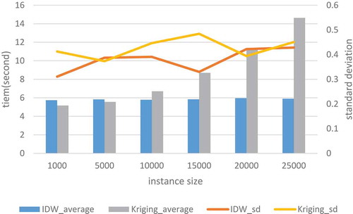
From Figure 5, the IDW interpolation is almost constant in terms of computational effort (less than 6 seconds) despite large problem sizes, while Kriging experiences sharp increases with larger datasets, confirming earlier computational findings presented by (Lam 1983).

5.2. Evaluation

Our web-based SDSS was specifically designed for environment health specialists with limited GIS background. To test the usefulness of iWWRE, an evaluation meeting was organized with an environmental health specialist from Gaston County, NC, who oversees the private wells program. During the meeting, the iWWRE interface was demonstrated using arsenic observations while interpolated maps for different time ranges were dynamically generated. We also demonstrated the flexibility of iWWRE for parameter calibration (power coefficient and search neighbourhood – resulting in slightly different maps) and cross validation results. After the presentation, an open-ended questionnaire was provided to gather feedback regarding the practicality of iWWRE.

Overall, it was recognized that the iWWRE Panel Component (including the dropdown menu to select the type of contaminant and the selection of temporal ranges) was easy to navigate, while the estimation maps were easy to interpret.

The environmental health specialist suggested that the interpolated maps of arsenic helped confirm beliefs about contamination patterns in the northwestern areas of the county (based on expert knowledge) while the MCL threshold lines were particularly useful to delineate the boundaries of the contamination. The specialist also mentioned that maps of contamination could provide evidence and result into guidelines to allocate additional resources for well testing and educate current and future well owners, especially in high-risk areas.

Although we organized our evaluation around arsenic contamination, we also demonstrated our system for nitrate contamination, and the specialist suggested possible linkages between farming and high nitrate concentration.

Despite these strengths, the specialist did not have knowledge on the parameters specific to the interpolation approach, nor a solid understanding on how to interpret cross-validation results. These two issues can be alleviated by providing a short training or a built-in section on how to calibrate parameters and interpret cross validation results. Secondly, the specialist suggested to have additional secondary layers, such as land-use information or the location of septic system that may help reveal detect a spatial association to certain contaminants. Lastly, it was suggested to add functionality that would lists users of private wells in areas deemed at risk for contamination.

5.3. Future research

There are several avenues that warrant future research. First, more spatial analysis functionality (e.g., overlay analysis, cluster analysis) will be incorporated as geoprocessing services to further enhance the spatially explicit estimation of water contamination risks. Second, our interpolation did not consider anisotropy, a property that spatial variation may exhibit significant difference along specific directions. In Gaston County, the spatial distribution of several rock types is along the southeast-northwest corridor, and the geology is known to affect inorganic contaminants, such as arsenic. Third, given that the location of well samples change through time, relying only on interpolation may bias the results. We anticipate our interface to include other models such as co-kriging, Bayesian maximum entropy (Christakos and Serre 2000) or spatial autologistic regression, which can handle secondary information such as bedrock geology, or well depth for instance (Owusu et al. 2020). We plan to expand our web-based SDSS to include such sophisticated models in the near future. Fourth, the number of samples available during a specific time period may be too low to make accurate prediction, and the temporal query could enforce a minimum number of observations. Fifth, we only were able to conduct an evaluation testing with one environmental health expert. Ideally, the approach set forth in this paper would benefit from more feedback, especially how this system could be used in a decision making context. Sixth, it would be particularly interesting to further capitalize on the concept of bootstrapping, and integrate that information and the one from KDE (density of wells) to develop a confidence indicator. Along the same vein, testing for type I & type II error could provide useful information on uncertainty (for instance a well user living in the ‘below threshold’ contour line but still showing high concentrations). Finally, provenance-aware capabilities (Wang et al. 2008) will be implemented to store settings for parameters and associated results for geoprocessing services and underlying scientific workflows by users.

Disclosure statement

No potential conflict of interest was reported by the authors.

Additional information

Funding

This work was supported by the National Center for Environmental Health [CDC-RFA-EH15-1507].

Notes

1. https://mndatamaps.web.health.state.mn.us/interactive/wells.html and https://mnwellindex.web.health.state.mn.us/

2. https://www.nj.gov/dep/dsr/pwta/

3. https://www.arcgis.com/apps/MapSeries/index.html?appid=c0d7daea497049c1a686d07dab7106e5

4. https://dnrmaps.wi.gov/H5/?viewer = Water_Use_Viewer

5. Residents may decide to test their water multiple times, especially following the installation of remediation services, like reserve osmosis.

6. OK does not reproduce either the histogram or the spatial variability as given by the variogram function (Yamamoto 2005).

7. When no time range is provided, the default is to incorporate data covering the entire time period under consideration.

8. The average distance to the k^th closest neighbours can be estimated in CrimeStat (Levine 2006) for instance, and are provided in Appendix Table A1.

9. These parameters were defined following careful analysis of the empirical variogram and can be found in Appendix Table A2.

10. ‘Clusters’ here denote areas where the interpolated arsenic values are above the EPA MCL

11. The running time is calculated from the time the user selects data to the time the routines have been executed.

Appendix A1

Table A1. Bandwidths for KDE maps, coinciding with the 10th nearest neighbour distance. Estimated in CrimeStat (Levine 2006).

Year	Bandwidth (metre)
2011	4,430
2012	4,072
2013	4,565
2014	4,381
2015	4,120
2016	3,295
2017	3,626
2011–2017	1,352 (shorter distance given a larger amount of observations)

Appendix A2

Table A2. Variogram parameters (unit of range: metre).

Year	n	range	nugget	sill
2011	159	5,448.206	0	0.00007808106
2012	184	7,265.88	0.00000200737	0.00000157424
2013	145	938	0.00001464448	0.00002880519
2014	159	6,146	0.00001519551	0.00002764214
2015	161	7,535	0.00000109114	0.00001502497
2016	219	11,439	0.00000076126	0.00000097363
2017	194	7,200	0.00000000000	0.00000626041
2011–2017	1235	4,957	0.00000728694	0.00001572318

References

- Armstrong, M. P., P. J. Densham, and G. Rushton. 1986. “Architecture for a Microcomputer Based Spatial Decision Support System.” In Proceedings of the 2nd International Symposium on Spatial Data Handling: 120–130.
- Best, B. D., P. N. Halpin, E. Fujioka, A. J. Read, S. S. Qian, L. J. Hazen, and R. S. Schick. 2007. “Geospatial Web Services within a Scientific Workflow: Predicting Marine Mammal Habitats in a Dynamic Environment.” Ecological Informatics 2 (3): 210–223. doi:10.1016/j.ecoinf.2007.07.007.
- Burdziej, J. 2012. “A Web-based Spatial Decision Support System for Accessibility Analysis—concepts and Methods.” Applied Geomatics 4 (2): 75–84. doi:10.1007/s12518-011-0057-x.
- Buschmann, J., M. Berg, C. Stengel, L. Winkel, M. L. Sampson, P. T. Kim Trang, and P. H. Viet. 2008. “Contamination of Drinking Water Resources in the Mekong Delta Floodplains: Arsenic and Other Trace Metals Pose Serious Health Risks to Population.” Environment International 34 (6): 756–764. doi:10.1016/j.envint.2007.12.025.
- Choi, J.-Y., B. A. Engel, and R. L. Farnsworth. 2005. “Web-based GIS and Spatial Decision Support System for Watershed Management.” Journal of Hydroinformatics 7 (3): 165–174. doi:10.2166/hydro.2005.0014.
- Christakos, G., and M. L. Serre. 2000. “BME Analysis of Spatiotemporal Particulate Matter Distributions in North Carolina.” Atmospheric Environment 34 (20): 3393–3406. doi:10.1016/S1352-2310(00)00080-7.
- Claudio, O., G. S. Silverman., D. S. Vinson., A. Bobyarchick., R. Paul., and E. Delmelle. 2020. A Spatial Autologistic Model to Predict the Presence of Arsenic in Private Wells Across Gaston County, North Carolina Using Geology, Well Depth, and pH Exposure and Health. DOI: 10.1007/s12403-020-00373-6
- Delmelle, E., C. Dony, I. Casas, M. Jia, and W. Tang. 2014. “Visualizing the Impact of Space-time Uncertainties on Dengue Fever Patterns.” International Journal of Geographical Information Science 28 (5): 1107–1127. doi:10.1080/13658816.2013.871285.
- Delmelle, E., E. C. Delmelle, I. Casas, and T. Barto. 2011. “HELP: A GIS-based Health Exploratory Analysis Tool for Practitioners.” Applied Spatial Analysis and Policy 4 (2): 113–137. doi:10.1007/s12061-010-9048-2.
- Delmelle, E. M., and P. Goovaerts. 2009. “Second-phase Sampling Designs for Non-stationary Spatial Variables.” Geoderma 153 (1–2): 205–216. doi:10.1016/j.geoderma.2009.08.007.
- Densham, P. J. 1991. “Spatial Decision Support Systems.” In Geographical Information Systems Vol. 1: Principles, D. J., Maguire, M., F., Goodchild, and D. W., Rhind, (Eds.)., pp. 403-412. Essex: Longman.
- Distefano, V., S. De Iaco, M. Palma, and A. Spennato. 2015. “Radon Risk Analysis through Geostatistical Tools Implemented in a WebGIS.” Current Air Quality Issues, 397.
- Dummer, T. J. B., Z. M. Yu, L. Nauta, J. D. Murimboh, and L. Parker. 2015. “Geostatistical Modelling of Arsenic in Drinking Water Wells and Related Toenail Arsenic Concentrations across Nova Scotia, Canada.” Science of the Total Environment 505: 1248–1258. doi:10.1016/j.scitotenv.2014.02.055.
- Dymond, R. L., B. Regmi, V. K. Lohani, and R. Dietz. 2004. “Interdisciplinary Web-enabled Spatial Decision Support System for Watershed Management.” Journal of Water Resources Planning and Management 130 (4): 290–300. doi:10.1061/(ASCE)0733-9496(2004)130:4(290).
- Elumalai, V., K. Brindha, B. Sithole, and E. Lakshmanan. 2017. “Spatial Interpolation Methods and Geostatistics for Mapping Groundwater Contamination in a Coastal Area.” Environmental Science and Pollution Research 24 (12): 11601–11617. doi:10.1007/s11356-017-8681-6.
- Esquivel, J. M., G. P. Morales, and M. V. Esteller. 2015. “Groundwater Monitoring Network Design Using GIS and Multicriteria Analysis.” Water Resources Management 29 (9): 3175–3194. doi:10.1007/s11269-015-0989-8.
- Fu, P., and J. Sun. 2010. Web GIS: Principles and Applications. Esri Press, Redlands, CA: Environmental Systems Research Institute.
- Gaus, I., D. G. Kinniburgh, J. C. Talbot, and R. Webster. 2003. “Geostatistical Analysis of Arsenic Concentration in Groundwater in Bangladesh Using Disjunctive Kriging.” Environmental Geology 44 (8): 939–948. doi:10.1007/s00254-003-0837-7.
- Ghosh, D. 2008. “A Loose Coupling Technique for Integrating GIS and Multi‐criteria Decision Making.” Transactions in GIS 12 (3): 365–375. doi:10.1111/j.1467-9671.2008.01103.x.
- Global Open Data Index. 2016. “Water Quality.” Accessed 07 November 2019. https://index.okfn.org/dataset/water/
- Gong, G., S. Mattevada, and S. E. O’Bryant. 2014. “Comparison of the Accuracy of Kriging and IDW Interpolations in Estimating Groundwater Arsenic Concentrations in Texas.” Environmental Research 130: 59–69. doi:10.1016/j.envres.2013.12.005.
- Goovaerts, P. 1997. Geostatistics for Natural Resources Evaluation. Oxford, NY: Oxford University Press on Demand.
- Goovaerts, P. 2017. “The Drinking Water Contamination Crisis in Flint: Modeling Temporal Trends of Lead Level since Returning to Detroit Water System.” Science of the Total Environment 581: 66–79. doi:10.1016/j.scitotenv.2016.09.207.
- Goovaerts, P., G. AvRuskin, J. Meliker, M. Slotnick, G. Jacquez, and J. Nriagu. 2005. “Geostatistical Modeling of the Spatial Variability of Arsenic in Groundwater of Southeast Michigan.” Water Resources Research 41: 7. doi:10.1029/2004WR003705.
- Hanna-Attisha, M., J. LaChance, R. C. Sadler, and A. C. Schnepp. 2016. “Elevated Blood Lead Levels in Children Associated with the Flint Drinking Water Crisis: A Spatial Analysis of Risk and Public Health Response.” American Journal of Public Health 106 (2): 283–290. doi:10.2105/AJPH.2015.303003.
- Hiemstra, P. H., E. J. Pebesma, C. J. W. Twenhöfel, and G. B. M. Heuvelink. 2009. “Real-time Automatic Interpolation of Ambient Gamma Dose Rates from the Dutch Radioactivity Monitoring Network.” Computers & Geosciences 35 (8): 1711–1721. doi:10.1016/j.cageo.2008.10.011.
- Hoover, J. H., P. C. Sutton, S. J. Anderson, and A. C. Keller. 2014. “Designing and Evaluating a Groundwater Quality Internet GIS.” Applied Geography 53: 55–65. doi:10.1016/j.apgeog.2014.06.005.
- Jankowski, P., M. Tsou, and R. D. Wright. 2007. “Applying Internet Geographic Information System for Water Quality Monitoring.” Geography Compass 1 (6): 1315–1337. doi:10.1111/j.1749-8198.2007.00065.x.
- Jung, C. D., and C. H. Sun. 2006. “Development of a Web-Based Spatial Decision Support System for Business Location Choice in Taipei City.” Proceeding of SPIE 6421. 2006 Esri International User Conference Proceedings on the website.
- Kelly, G. C., C. M. Seng, W. Donald, G. Taleo, J. Nausien, W. Batarii, H. Iata, M. Tanner, L. S. Vestergaard, and A. C. A. Clements. 2011. “A Spatial Decision Support System for Guiding Focal Indoor Residual Spraying Interventions in A Malaria Elimination Zone.” Geospatial Health 6: 21–31. doi:10.4081/gh.2011.154.
- Kienberger, S., M. Hagenlocher, E. Delmelle, I. Casas, and M. Hagenlocher. 2013. “A WebGIS Tool for Visualizing and Exploring Socioeconomic Vulnerability to Dengue Fever in Cali, Colombia.” Geospatial Health 8 (1): 313–316. doi:10.4081/gh.2013.76.
- Kim, D., M. L. Miranda, J. Tootoo, P. Bradley, and A. E. Gelfand. 2011. “Spatial Modeling for Groundwater Arsenic Levels in North Carolina.” Environmental Science & Technology 45 (11): 4824–4831. doi:10.1021/es103336s.
- Lam, N. S.-N. 1983. “Spatial Interpolation Methods: A Review.” The American Cartographer 10 (2): 129–150. doi:10.1559/152304083783914958.
- Levine, N. 2006. “Crime Mapping and the Crimestat Program.” Geographical Analysis 38 (1): 41–56. doi:10.1111/j.0016-7363.2005.00673.x.
- Li, W., L. Linna, M. Goodchild, and L. Anselin. 2013. “A Geospatial Cyberinfrastructure for Urban Economic Analysis and Spatial Decision-making.” ISPRS International Journal of Geo-Information 2 (2): 413–431. doi:10.3390/ijgi2020413.
- Lin, T., S. Wang, L. F. Rodríguez, H. Hao, and Y. Liu. 2015. “CyberGIS-enabled Decision Support Platform for Biomass Supply Chain Optimization.” Environmental Modelling & Software 70: 138–148. doi:10.1016/j.envsoft.2015.03.018.
- Liu, A., J. Ming, and R. O. Ankumah. 2005. “Nitrate Contamination in Private Wells in Rural Alabama, United States.” Science of the Total Environment 346 (1–3): 112–120. doi:10.1016/j.scitotenv.2004.11.019.
- Maharjan, M., C. Watanabe, S. A. Ahmad, and R. Ohtsuka. 2005. “Arsenic Contamination in Drinking Water and Skin Manifestations in Lowland Nepal: The First Community-based Survey.” The American Journal of Tropical Medicine and Hygiene 73 (2): 477–479. doi:10.4269/ajtmh.2005.73.477.
- Malczewski, J. 1999. GIS and Multicriteria Decision Analysis. Newyork, NY: John Wiley & Sons.
- Meliker, J. R., G. A. AvRuskin, M. J. Slotnick, P. Goovaerts, D. Schottenfeld, G. M. Jacquez, and J. O. Nriagu. 2008. “Validity of Spatial Models of Arsenic Concentrations in Private Well Water.” Environmental Research 106 (1): 42–50. doi:10.1016/j.envres.2007.09.001.
- Mirzaei, R., and M. Sakizadeh. 2016. “Comparison of Interpolation Methods for the Estimation of Groundwater Contamination in Andimeshk-Shush Plain, Southwest of Iran.” Environmental Science and Pollution Research 23 (3): 2758–2769. doi:10.1007/s11356-015-5507-2.
- Modica, G., M. Pollino, S. Lanucara, L. La Porta, G. Pellicone, S. D. Fazio, and C. R. Fichera. 2016. “Land Suitability Evaluation for Agro-forestry: Definition of a Web-based Multi-criteria Spatial Decision Support System (MC-SDSS): Preliminary Results.” In International Conference on Computational Science and Its Applications: 399-413. Springer, Cham.
- Murray, R., J. Uber, and R. Janke. 2006. “Model for Estimating Acute Health Impacts from Consumption of Contaminated Drinking Water.” Journal of Water Resources Planning and Management 132 (4): 293–299. doi:10.1061/(ASCE)0733-9496(2006)132:4(293).
- Mwaura, D., and M. Kada. 2017. “Developing a Web-based Spatial Decision Support System for Geothermal Exploration at the Olkaria Geothermal Field.” International Journal of Digital Earth 10 (11): 1118–1145. doi:10.1080/17538947.2017.1284909.
- Nas, B., and A. Berktay. 2010. “Groundwater Quality Mapping in Urban Groundwater Using GIS.” Environmental Monitoring and Assessment 160 (1–4): 215–227. doi:10.1007/s10661-008-0689-4.
- Nobre, R. C. M., O. C. Rotunno Filho, W. J. Mansur, M. M. M. Nobre, and C. A. N. Cosenza. 2007. “Groundwater Vulnerability and Risk Mapping Using GIS, Modeling and a Fuzzy Logic Tool.” Journal of Contaminant Hydrology 94 (3–4): 277–292. doi:10.1016/j.jconhyd.2007.07.008.
- Olea, R. A., and V. Pawlowsky. 1996. “Compensating for Estimation Smoothing in Kriging.” Mathematical Geology 28 (4): 407–417. doi:10.1007/BF02083653.
- Owusu, C., Y. Lan, M. Zheng, W. Tang, and E. Delmelle. 2017. “Geocoding Fundamentals and Associated Challenges.” Geospatial Data Science Techniques and Applications 41–62. Boca Raton, LA: Taylor and Francis Group.
- Pebesma, E., D. Cornford, G. Dubois, G. B. M. Heuvelink, D. Hristopulos, J. Pilz, U. Stöhlker, G. Morin, and J. O. Skøien. 2011. “INTAMAP: The Design and Implementation of an Interoperable Automated Interpolation Web Service.” Computers & Geosciences 37 (3): 343–352. doi:10.1016/j.cageo.2010.03.019.
- Peng, Z.-R., and M.-H. Tsou. 2003. Internet GIS: Distributed Geographic Information Services for the Internet and Wireless Networks. Hoboken, NJ: John Wiley & Sons.
- Preziosi, E., A. B. Petrangeli, and G. Giuliano. 2013. “Tailoring Groundwater Quality Monitoring to Vulnerability: A GIS Procedure for Network Design.” Environmental Monitoring and Assessment 185 (5): 3759–3781. doi:10.1007/s10661-012-2826-3.
- Rahman, M. 2002. “Arsenic and Contamination of Drinking-water in Bangladesh: A Public-health Perspective.” Journal of Health, Population and Nutrition 20(3): 193–197.
- Ries, I. I. I., G. Kernell, J. G. Guthrie, A. H. Rea, P. A. Steeves, and D. W. Stewart. 2008. “StreamStats: A Water Resources Web Application.” US Geological Survey Fact Sheet 3067 (6): 12018–3003.
- Rogan, W. J., and M. T. Brady. 2009. “Drinking Water from Private Wells and Risks to Children.” Pediatrics 123 (6): e1123–e37. doi:10.1542/peds.2009-0752.
- Rogerson, P. A., E. Delmelle, R. Batta, M. Akella, A. Blatt, and G. Wilson. 2004. “Optimal Sampling Design for Variables with Varying Spatial Importance.” Geographical Analysis 36 (2): 177–194. doi:10.1111/j.1538-4632.2004.tb01131.x.
- Samadder, S. R., and C. Subbarao. 2007. “GIS Approach of Delineation and Risk Assessment of Areas Affected by Arsenic Pollution in Drinking Water.” Journal of Environmental Engineering 133 (7): 742–749. doi:10.1061/(ASCE)0733-9372(2007)133:7(742).
- Schäjfler, U., D. Moraru, C. Heier, K.-H. Spies, and M. Schilcher. 2010. “Interpolation of Precipitation Sensor Measurements Using OGC Web Services.” In Proceedings of EnviroInfo 2010, edited by Klaus Greve and Armin B. Cremers, 549–555. Aachen: Shaker.
- Shrestha, R. R., M. P. Shrestha, N. P. Upadhyay, R. Pradhan, R. Khadka, A. Maskey, M. Maharjan, S. Tuladhar, B. M. Dahal, and K. Shrestha. 2003. “Groundwater Arsenic Contamination, Its Health Impact and Mitigation Program in Nepal.” Journal of Environmental Science and Health, Part A 38 (1): 185–200. doi:10.1081/ESE-120016888.
- Strauss, B., W. King, A. Ley, and J. R. Hoey. 2001. “A Prospective Study of Rural Drinking Water Quality and Acute Gastrointestinal Illness.” BMC Public Health 1 (1): 8. doi:10.1186/1471-2458-1-8.
- Sugumaran, R., and J. Degroote. 2010. Spatial Decision Support Systems: Principles and Practices. Boca Raton, FL: Crc Press.
- Sugumaran, R., J. C. Meyer, and J. Davis. 2004. “A Web-based Environmental Decision Support System (WEDSS) for Environmental Planning and Watershed Management.” Journal of Geographical Systems 6 (3): 307–322. doi:10.1007/s10109-004-0137-0.
- Tang, W., W. Feng, M. Jia, J. Shi, H. Zuo, C. E. Stringer, and C. C. Trettin. 2017. “A Cyber-enabled Spatial Decision Support System to Inventory Mangroves in Mozambique: Coupling Scientific Workflows and Cloud Computing.” International Journal of Geographical Information Science 31 (5): 907–938. doi:10.1080/13658816.2016.1245419.
- Tomczak, M. 1998. “Spatial Interpolation and Its Uncertainty Using Automated Anisotropic Inverse Distance Weighting (Idw)-cross-validation/jackknife Approach.” Journal of Geographic Information and Decision Analysis 2 (2): 18–30.
- U.S. EPA. “Private Drinking Water Wells.” Accessed 30 March 2019. https://www.epa.gov/privatewells
- Wang, S. 2010. “A CyberGIS Framework for the Synthesis of Cyberinfrastructure, GIS, and Spatial Analysis.” Annals of the Association of American Geographers 100 (3): 535–557. doi:10.1080/00045601003791243.
- Wang, S., A. Padmanabhan, J. D. Myers, W. Tang, and Y. Liu. 2008. “Towards Provenance-aware Geographic Information Systems.” Paper presented at the Proceedings of the 16th ACM SIGSPATIAL international conference on Advances in geographic information systems, Irvine, CA, USA.
- Whitacre, D. M. 2009. Reviews of Environmental Contamination and Toxicology. Vol. 202. Springer, New York: Springer.
- Williams, M., D. Cornford, L. Bastin, R. Jones, and S. Parker. 2011. “Automatic Processing, Quality Assurance and Serving of Real-time Weather Data.” Computers & Geosciences 37 (3): 353–362. doi:10.1016/j.cageo.2010.05.010.
- Wongsasuluk, P., S. Chotpantarat, W. Siriwong, and M. Robson. 2014. “Heavy Metal Contamination and Human Health Risk Assessment in Drinking Water from Shallow Groundwater Wells in an Agricultural Area in Ubon Ratchathani Province, Thailand.” Environmental Geochemistry and Health 36 (1): 169–182. doi:10.1007/s10653-013-9537-8.
- Yamamoto, J. K. 2005. “Correcting the Smoothing Effect of Ordinary Kriging Estimates.” Mathematical Geology 37 (1): 69–94. doi:10.1007/s11004-005-8748-7.
- Yang, C., R. Raskin, M. Goodchild, and M. Gahegan. 2010. “Geospatial Cyberinfrastructure: Past, Present and Future.” Computers, Environment and Urban Systems 34 (4): 264–277. doi:10.1016/j.compenvurbsys.2010.04.001.
- Yao, X., D. Zhu, W. Yun, F. Peng, and L. Lin. 2017. “A WebGIS-based Decision Support System for Locust Prevention and Control in China.” Computers and Electronics in Agriculture 140: 148–158. doi:10.1016/j.compag.2017.06.001.
- Zeng, Y., Y. Cai, P. Jia, and H. Jee. 2012. “Development of a Web-based Decision Support System for Supporting Integrated Water Resources Management in Daegu City, South Korea.” Expert Systems with Applications 39 (11): 10091–10102. doi:10.1016/j.eswa.2012.02.065.
- Zhang, C., T. Zhao, and L. Weidong. 2010. “The Framework of a Geospatial Semantic Web-based Spatial Decision Support System for Digital Earth.” International Journal of Digital Earth 3 (2): 111–134. doi:10.1080/17538940903373803.
- Zhang, Z., H. Hao, D. Yin, S. Kashem, L. Ruopu, H. Cai, D. Perkins, and S. Wang. 2019. “A cyberGIS-enabled Multi-criteria Spatial Decision Support System: A Case Study on Flood Emergency Management.” International Journal of Digital Earth 12 (11): 1364–1381. doi:10.1080/17538947.2018.1543363.