Choosing an appropriate training set size when using existing data to train neural networks for land cover segmentation

ABSTRACT

Land cover data is an inventory of objects on the Earth’s surface, which is often derived from remotely sensed imagery. Deep Convolutional Neural Network (DCNN) is a competitive method in image semantic segmentation. Some scholars argue that the inadequacy of training set is an obstacle when applying DCNNs in remote sensing image segmentation. While existing land cover data can be converted to large training sets, the size of training data set needs to be carefully considered. In this paper, we used different portions of a high-resolution land cover map to produce different sizes of training sets to train DCNNs (SegNet and U-Net) and then quantitatively evaluated the impact of training set size on the performance of the trained DCNN. We also introduced a new metric, Edge-ratio, to assess the performance of DCNN in maintaining the boundary of land cover objects. Based on the experiments, we document the relationship between the segmentation accuracy and the size of the training set, as well as the nonstationary accuracies among different land cover types. The findings of this paper can be used to effectively tailor the existing land cover data to training sets, and thus accelerate the assessment and employment of deep learning techniques for high-resolution land cover map extraction.

KEYWORDS:

• Land Cover
• deep Learning
• edge-ratio
• training set
• image semantic segmentation

1. Introduction

Land cover data represent contiguous objects on the Earth’s surface, such as forest, waterbody, croplands, or residential area. Since land cover reflects the potential use value of the land resource, land cover data is valuable for the administrative authorities to evaluate, plan, use, manage, and monitor natural resources. For example, in the county-level administration, land cover data based on high-resolution images from 0.5 to 2 m (Ma et al. 2017) are commonly used to represent micro-landscape and provide accurate fundamental data for precise municipal administration.

Typically, land cover data contains land cover maps and corresponding remote sensing (RS) imagery. The land cover map is extracted from the RS images automatically or manually. Numerous historical land cover data have been accumulated from the monitoring activities by local authorities. For example, each county in China has produced a land cover map based on the sub-metre RS images manually in the National Geoinformation Survey from 2013 to 2017 (Xinhua 2017). In the United States, the Iowa Department of Natural Resources released a land cover raster layer of 1-metre resolution based on a pixel-wise classification approach (Iowa Department of Natural Resources 2009).

Deep learning, or multiple-layer artificial neural network, is a recently adopted approach of machine learning in remote sensing domain (Zhu et al. 2017), providing a promising method to automatic extraction of land cover products. Among various machine learning approaches, the deep convolutional neural network (DCNN) has been commonly used (Liu et al. 2017; McCann, Jin, and Unser 2017). DCNNs are hungry for large-scale training datasets. In the computer vision domain, large open datasets are the cornerstones of deep learning. For example, the well-known ImageNet (Russakovsky et al. 2015) contains over 14 million annotated images in 1,000 classes. The Common Objects in Context (COCO) dataset is a large-scale dataset for object detection, segmentation, and captioning (Lin et al. 2014). COCO includes 328,000 images, 2,500,000 labelled instances, and 91 object categories, most of which have more than 5,000 labelled instances.

Researchers in remote sensing community have argued that the lack of training sets is one of the main concerns when applying DCNN. Ball, Anderson, and Chan (2017) reviewed over 260 deep learning related remote sensing articles and ranked the data inadequacy as the first of the unsolved challenges for deep learning in remote sensing. Ball, Anderson, and Wei (2018) listed transfer learning, unsupervised learning, and generative adversarial network (Goodfellow et al. 2014) as the promising solutions for the lack of training data in the remote sensing research. The small study areas in most research articles reflect this insufficiency of training sets. Ma et al. (2019) share similar views in a review article that most land cover and land use studies used a single small image scene.

Though some scholars argue the eagerness of DCNN for large training sets is difficult to be satisfied in a short period (Ball, Anderson, and Chan 2017; Ball, Anderson, and Wei 2018; Ma et al. 2019), we believe that this challenge can be tackled by converting the existing land cover datasets into training sets: the land cover maps are used as the labels, and the associated images as the samples. In this regard, most of land cover data users, such as land managers, urban planners, and researchers, can use their previous data to train a model to produce land cover maps from new images.

When converting existing land cover datasets to training sets for deep learning applications, various aspects need to be considered, such as the size of training set, imbalance of categories, and sampling strategy. While large training set often leads to a better performance for DCNNs (Zhu et al. 2016), the computing time and resources used also increase accordingly. Thus, the size of training data set needs to be carefully considered. How big of the training set size is big enough for an application? What is the impact of the size of the training set on the accuracy of segmentation results? Is the accuracy consistent among different land cover types and landscapes (e.g., urban vs. rural area)? If not, what does the role of training set size play in such variations? These are essential questions to ask when leveraging existing land cover maps and RS images to build deep learning training sets. To shed light on seeking answers to these questions, our study focuses on evaluating the impact of training set size on the model performance quantitatively, and then provides guidelines for choosing an appropriate size.

To explore the relationship between the training set size and the performance of DCNN, this paper used different portions of a county-level land cover dataset with 0.5 m RS images to form different sizes of training sets, and then compared the land cover extraction results using two DCNNs (SegNet and U-Net) trained with different training set sizes. Besides, we introduced a new metric of Edge-ratio, the percentage of pixels on edge, to evaluate performances of DCNNs in the object boundary. The findings of this paper can help effectively tailor the existing land cover data to training sets, and thus accelerate the assessment and employment of deep learning techniques for high-resolution land cover map extraction.

2. Related work

DCNNs have been applied on land cover domain in recent years. Scott et al. (2017) trained and fused three DCNNs (CaffeNet, GoogLeNet, and ResNet50) for land cover extraction from high-resolution imagery. The fusion model reached the accuracies of 99.3% for UC Merced Land Use Dataset (Yang and Newsam 2010) and 99.2% for another (Dai and Yang 2011) dataset of 19 classes. Huang, Zhao, and Song (2018) used a semi-transfer DCNN to map urban land use from the metre-scale satellite images and obtained overall accuracy of 80–91%. Sherrah (2016) applied a fully convolutional network (FCN, Long, Shelhamer, and Darrell 2015) to semantically segment the ISPRS Vaihingen and Potsdam datasets (Rottensteiner et al. 2012) of sub-decimetre resolution at an accuracy of 89.7%.

In most deep learning studies on land cover, the sizes of the training sets are small. These small datasets may be insufficient to train a DCNN. According to Ma et al. (2017), 95.6% of research areas in published articles are less than 300 ha and use small training sets. Many studies involving DCNNs used small training sets too. Zhang et al. (2018) conducted an object-based convolutional neural network for urban land use classification based on only two images of about 6,000 × 5,000 pixels (0.5 m resolution). Längkvist et al. (2016) used an orthographic image of 12,648 × 12,736 pixels (0.5 m resolution) to investigate several DCNN architectures for classification and segmentation. To our best knowledge, there is no DCNN-based land cover research using large datasets such as those in the county level. Therefore, the performance of the DCNN may not be sufficiently evaluated in aforementioned research.

On the other hand, many existing high-resolution images and land cover data are available from historical applications, and these data can be, leveraged to build large training sets. Some scholars have used publicly accessible GIS data, such as Open Street Map (OSM, Haklay and Weber 2008), as land cover labels for RS images classification and segmentation (Luo et al. 2019; Grippa et al. 2018; Ghaffarian et al. 2019; Audebert, Le Saux, and Lefevre 2017; Zhao et al. 2019). Existing land cover maps of a medium resolution can be also updated by OSM data (Fonte et al. 2017). These studies have explored the feasibility of reusing land cover data or OSM data as training sets, but the methods of reusing were not elaborated. Therefore, we investigate the conversion from land cover data to training sets.

Some studies noticed that the sampling method to form the training set and test set impacts the test result (Zhen et al. 2013; Jin, Stehman, and Mountrakis 2014), but they did not consider the size of the training set. Heydari and Mountrakis (2018) conducted experiments to explore the effects of the size of the training set. Using Landsat imagery and six pixel-wise classification methods, the researchers sampled the land cover data by 5%, 2%, and 0.2% to assess the effect of the sample size. Twenty-six 10 km×10 km images with 30 m resolution in total were tested. The authors reported a declining trend in the best attainable accuracy when downsizing the training set, but the accuracy of 5% size sample is close to the 2% size sample. Inspired by the research by Heydari and Mountrakis (2018), our research investigates the impact of training set size on the DCNN model performance, using a large dataset.

3. Data and methods

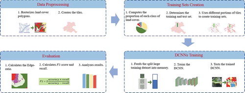
The overall research workflow is illustrated in Figure 1, which includes four major steps. The first step is data preprocessing, which first rasterizes the land cover vector layer to a land cover image and then splits this image into smaller tiles. The RS images used to extract the land cover vector are divided with the same schema. In the second step, six training sets are formed by the different portions of the tiles, and one test set is created. Two popular architectures of DCNN in image segmentation, SegNet (Badrinarayanan, Kendall, and Cipolla 2017) and U-Net (Ronneberger, Fischer, and Brox 2015), are trained in the third step, and the trained DCNNs are used to segment the test set semantically. Lastly, the segmentation results of the test set are evaluated and compared.

Figure 1. The overall workflow of the experiment

2.1. Data preprocessing

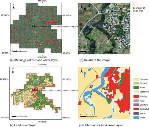
We select Dongxiang County, Jiangxi Province, China, as the study area, covering about 900 km². The experimental data includes a county-level land cover polygon layer derived from a set of aerial images of 0.5 m resolution acquired in the autumn of 2014. The land cover layer contains about 70,000 manually drawn polygons. Figure 2(a,c) shows the RS images and the land cover layer of the entire research area, respectively. Figure 2(b,d) shows a zoom-in view of the RS image and land cover layer, respectively. The land cover layer was coded into ten classes using photo interpretation: Cropland, Grassland, Orchard, Forest, Housing Area, Road, Structure, Water, Barren Land, and Excavated Land. Structure means constructions do not have human living functions, such as dams and water towers. Excavated Land refers to the land exposed by sizable civil engineering projects (e.g., open mining site, construction site). According to Figure 2, most of Housing Areas cluster in the central part of Dongxiang County, surrounding by Cropland. Forest is located in the periphery of the county.

Due to the generalization, some small areas were mixed up to dominated land cover types nearby, especially the Housing Area and Cropland classes. For instance, the open space between the buildings was included in the Housing Area. The objects inside a land cover polygon may not be homogeneous, which means DCNNs may need more examples to learn the rule to segment those heterogeneous textures.

Figure 2. The experimental dataset

Usually, a training set for image semantic segmentation contains two types of data: images and labels in raster format. Each pixel in the image requires a corresponding label in the label raster. We rasterized the 10-class land cover polygons into a land cover map, which is used as the label image. The image and label was split in 146 tiles of 5,000 × 5,000 pixels, respectively.

2.2. Training sets creation

To test how the performance of DCNNs is affected by the size of the training set in the land cover application, six training sets were created using different numbers of tiles: 20, 40, 60, 80, 100, and 120 (Figure 3). The performance of the DCNN from the largest training set (120 tiles) was used as the baseline. DCNNs are trained by smaller training sets, and their performances are compared with the baseline.

The proportion of classes varies in the study area. Forest is the largest class, accounting for 45.61%, followed by Cropland of 31.12%. Barren, Structure, Road, and Excavated Land have a small portion, ranging from 0.02% to 1.70%. Also, polygon sizes vary dramatically. A Forest polygon may cover a large hill, while a Housing Area polygon may merely cover a small house. To reduce the potential biases in training sets, we evenly selected 20 tiles to form the first training set, which has a similar class distribution as the entire land cover dataset. We then built the second training set by adding 20 adjacent tiles to the first training set and added another 20 adjacent tiles to the second training set to form the third training set, and so on. Finally, six training sets were created with a similar class distribution.

The test set has 26 tiles. These tiles cover typical areas of the research site, containing the urban area to the mountain in the suburbs. Because the portion of Barren is small (0.02%) and its geographic distribution is not even, we do not access the model performance on Barren. Overall, the six training sets and test set share a similar class distribution (Table 1), so that there is no bais caused by different class distributions among datasets when training and testing.

Table 1. Training sets and test set sharing a similar class distribution

Dataset	Test	20	40	60	80	100	120	Total
Cropland	27.01%	31.77%	32.66%	33.97%	32.90%	32.30%	31.76%	31.12%
Orchard	2.92%	2.33%	2.60%	2.83%	2.80%	2.84%	2.68%	2.71%
Forest	49.97%	46.93%	45.32%	43.36%	43.58%	44.32%	44.91%	45.61%
Grassland	5.18%	5.39%	5.53%	5.73%	5.86%	5.74%	5.67%	5.60%
Housing Area	4.96%	4.35%	4.40%	4.65%	4.85%	5.05%	5.43%	5.35%
Road	1.64%	1.20%	1.20%	1.37%	1.41%	1.43%	1.50%	1.51%
Structure	0.80%	0.58%	0.71%	0.77%	0.78%	0.76%	0.79%	0.80%
Excavated Land	1.94%	1.41%	1.56%	1.62%	1.73%	1.79%	1.67%	1.70%
Barren	0.02%	0.04%	0.02%	0.02%	0.03%	0.03%	0.03%	0.02%
Water	5.56%	5.99%	5.99%	5.69%	6.06%	5.73%	5.57%	5.57%

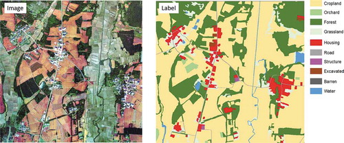
We cropped the entire RS image of the study area into tiles. Each land cover tile has an associated image with the same dimension (5,000 × 5,000 pixels) and location. When training, the images serve as the input of the model, and the land cover maps serve as labels. Figure 4 shows a sample (1/4 tile) in the training sets.

Figure 3. Training set and test set (26 tiles)

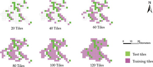
Figure 4. An example (1/4 tile) in the training set

2.3. DCNNs training

We adapted DeepNetsForEO (Audebert, Le Saux, and Lefèvre 2018) as the experimental framework. DeepNetsForEO is based on SegNet (Badrinarayanan, Kendall, and Cipolla 2017). SegNet is an Encoder-Decoder architecture, and it retains the small objects in the output feature map using up-sampling layers (Figure 5). The Encoder of SegNet has five convolution blocks with each block consisting of 2 or 3 convolutional layers. All the kernels are 3 × 3 with a padding of 1. The activate function is ReLU (Rectified Linear Unit), and the Batch Normalization (BN) (Ioffe and Szegedy 2015) is applied. After five max-pooling layers of 2 × 2 in each block, the size of the feature map is reduced to 1/32 of the input image. The Decoder up-samples the feature map into the original image size. Five un-pooling layers (Zeiler and Fergus 2014) in the Decoder relocate the activations according to the indices recorded in the pooling processes. At the end of the Decoder, a soft-max layer generates the predicted label from the dense prediction.

Figure 5. SegNet architecture

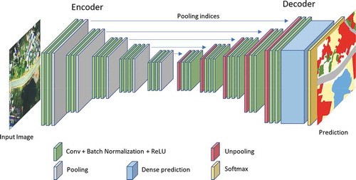
U-Net (Ronneberger, Fischer, and Brox 2015) is similar to SegNet. The main difference is that the outputs of each block are concatenated to the counterpart in the Decoder (skip-connection). In this study, five blocks are utilized, and all the convolution kernels are 3 × 3 and the paddings are one. This U-Net implementation was added to DeepNetsForEO.

In DeepNetsForEO, the size of the input image is 256 × 256 pixels. During the training process, the framework randomly picks a tile and cropping a patch of 256 × 256 pixels in a random position then push this patch into a sample batch. Hence, the samples in a batch come from different tiles covering various landscapes. When training, if these patches come from the same tile, which only covers a small area, they may have a similar texture, then mislead the descent direction of the gradient and fluctuate the loss, eventually affect the performances of models.

During the training process, the same hyper-parameters were employed to all the training sets: a base learning rate of 0.01, a momentum of 0.9, and a weight decay of 0.0005. The batch size was set to 40. The initial weights of Encoder were fed with VGG-16 trained by ImageNet. The base learning rate multiplied a factor of 0.1 after 15, 25, 35, and 45 epochs. When training, models’ losses were stable after about 30 epochs, so that we trained the models 50 epochs. Hence, the test results from these sufficiently trained models can reflect the impact of the size of training sets. The test environment includes Ubuntu 16.04, PyTorch and Jupyter notebook. The computer workstation consists of two Nvidia Titan Xp graph cards (12 GB memory each), one Intel i7 CPU, 1.5 T SSD, and 64GB memory.

2.4. Evaluation metrics and edge-ratio

We trained DCNN with six training sets and then used the trained DCNNs to classify the test set of 26 tiles. Accuracy, Cohen’s kappa, and F1 score were applied to evaluate the segmentation results. Accuracy equals to the correct pixels divided by the total pixels (Equation (1))(1) $accuracy=\frac{truepositive+truengeative}{\begin{array}{c}truepositive+falsepositive\\ +falsenegative+truenegative\end{array}}$(1) . Cohen’s kappa is calculated with Equation (4)(4) $\kappa =\frac{p_o-p_e}{1-p_e}=1-\frac{1-p_o}{1-p_e}$(4) , where $p_o$ is equal to the accuracy, and $p_e$ is the hypothetical probability of chance agreement calculated with Equation (5)(5) $p_e=\frac{1}{N^2}\sum _k{n}_{k1}{n}_{k2}$(5) . N is the number of all pixels. For class k, $n_{k1}$ is the number of pixels in the ground truth, and $n_{k2}$ is the number of pixels in the predicted result. F1 score was calculated by Equation (6)(6) $F1=2\times \frac{precision\times recall}{precision-recall}$(6) , as a harmonic average of the precision (Equation (2))(2) $precision=\frac{truepositive}{truepositive+falsepositive}$(2) and recall (Equation (3))(3) $recall=\frac{truepositive}{truepositive+falsenegative}$(3) .

(1) $accuracy=\frac{truepositive+truengeative}{\begin{array}{c}truepositive+falsepositive\\ +falsenegative+truenegative\end{array}}$(1)

(2) $precision=\frac{truepositive}{truepositive+falsepositive}$(2)

(3) $recall=\frac{truepositive}{truepositive+falsenegative}$(3)

(4) $\kappa =\frac{p_o-p_e}{1-p_e}=1-\frac{1-p_o}{1-p_e}$(4)

(5) $p_e=\frac{1}{N^2}\sum _k{n}_{k1}{n}_{k2}$(5)

(6) $F1=2\times \frac{precision\times recall}{precision-recall}$(6)

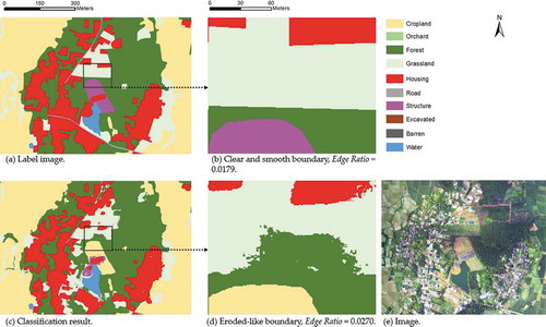
The widely used accuracy, kappa, and F1 score do not consider the spatial patterns of the segmentation result and therefore the eroded-like boundary, a common phenomenon in the segmentation algorithm, cannot be assessed. We propose a new metric, Edge-ratio, to better evaluate the results for the class boundary. Edge-ratio refers to the percentage of the pixels at the edge, which can be calculated with Equation (7)(7) $Edgeratio=\frac{numberofpixelsattheedge}{numberofallpixels}$(7) .

(7) $Edgeratio=\frac{numberofpixelsattheedge}{numberofallpixels}$(7)

In a land cover map, if a pixel has a neighbour on the right or down side was labelled as a different category, this pixel is defined as an edge pixel. Edge-ratio represents the complexity of the boundary. If a classifier smoothly depicts the object boundary on the test set, the Edge-ratios of the results and the test set should be close. Thus, the Edge-ratio can be used to evaluate the performance of a classifier on boundary delineation. Edge-ratio is also a reasonable indicator to show the potential improvement between the result and the ground truth. When the results from different classifiers have similar content but different boundaries, the one with the closest Edge-ratio to the label image should be preferred.

Figure 6 depicts the different boundaries of the label image and segmentation result. Typically, the label image has a clear and smooth boundary with a low Edge-ratio, and the segmentation result has an eroded-like boundary with a high Edge-ratio. To accurately explore the Edge-ratio and the performances of DCNNs, no post-process (e.g. smoothing) was applied to the results from the trained DCNNs in this study.

Figure 6. Edge Ratio in the label image and the segmentation result

4. Results

SegNet and U-Net were trained by the six training sets of 20, 40, 60, 80, 100, and 120 tiles, respectively, which were then applied to segment images in the test set. In our workstation, each tile (5,000 × 5,000 pixels) needs 10 minutes to be trained and needs 5 minutes to be segmented and evaluated (1.5 minutes to calculate the accuracy and F1 score). About 24 hours were needed to train and assess the baseline training set (120 tiles).

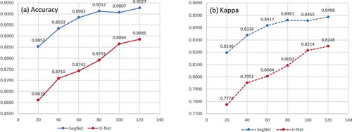
When using the baseline training set (120 tiles), both SegNet and U-Net obtained the highest performance. Visually, these results show a slight difference comparing with the label image. As shown in Figure 7, the accuracies and kappas from SegNet and U-Net share an increasing trend when increasing the training set. These figures indicate that larger training sets have higher performances. However, the performance increase rate declines and gradually levelled off for SegNet.

When the size of the training set is 100 tiles, the performance of SegNet is slightly lower than the size of 80 tiles (0.9012 and 0.9007, respectively), as well as kappa. The reason may be that SegNet is sufficiently trained when using a training set larger than 80 tiles, and the performance happens to go backward after the last batch of the 50th epochs. Normally, the model performance is fluctuant and is not guaranteed to be better after each training step. We save the model after 50 epochs rather than the model with the best performance in the training process. Therefore, all models were trained by 50 epochs and can be compared fairly with fewer variables.

Figure 7. Accuracies and kappas of different sizes of training sets

The F1 scores of the classes represent a similar increasing trend, along with the upsizing of the training set (Figure 8). The F1 scores of Water, Forest, Cropland, and Housing Area increase slowly, while Road, Structure Grass, and Orchard have a more significant increase. This is explained when looking into the details of the class image (Figure 9), the boundary of the urban area (Housing Area and Road) was significantly improved when increased the training set. In the result of the largest training set of 120 tiles, Water, Forest, and Cropland obtained relatively high F1 scores, followed by Road. Structure, Orchard, Grass, and Excavated Land got low F1 scores less than 0.5. Still, SegNet and U-Net show a similar trend while U-Net has lower performance.

Figure 8. F1 scores of each class. Columns from left to right in each cluster of classes represent training sets from 20 tiles to 120 tiles. SegNet (a) and U-Net (b) show a similar increasing trend when increasing the training set

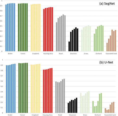
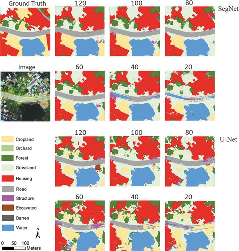
Figure 9. A sample of segmentation results of different training sets. In the results of small training sets (20 and 40 tiles), the pixels near the boundary are discrete, especially the Road class

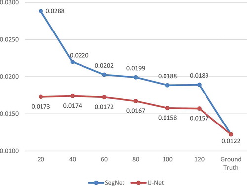
The Edge-ratios of the segmentation results show a clear decrease when enlarging the training set (Figure 10). For SegNet, it drops dramatically from 0.0288 to 0.0189 when the training set increases from 20 tiles to 120 tiles, but it is still larger than the Edge-ratio of the ground truth (0.0122, test set). U-Net returns smooth boundaries, and also obtains lower Edge-ratio when being trained by larger training sets. Similar to SegNet, the result of U-Net from 120 tiles has a gap to the ground truth on Edge-ratio.

Figure 10. Edge-ratios of segmentation results and the ground truth

5. Discussion

The results from SegNet and U-Net demonstrate that a larger training set leads to higher accuracy. However, the decrease is not significant when using smaller training sets. In our case, when using 20 tiles to train SegNet, the accuracy only dropped 0.0174, from 0.9027 (120 tiles) to 0.8853. Considering 6 times of saving on resource consumption (e.g., training time and data management), this small decrease may be acceptable for some time-sensitive applications such as disaster responses. U-Net gained more improvement from larger training sets, but its accuracy and kappa are significantly behind SegNet. The complexity of neural networks may play a role in the difference in performances. In our implementation, SegNet has about 29.4 million parameters, while U-Net has 19.4 million. However, the performance of DCNNs may vary among datasets and training strategies. The applicability of different architectures needs further investigation.

When examining the details of the segmentation results in the urban area (Figure 11), the boundaries of the classes obtained a significant degradation with smaller training sets from SegNet. When using small training sets (20, 40, and 60 tiles), there are discrete pixels near the class boundaries in the urban area, which indicates that the DCNN was insufficiently trained in the context-rich urban area. On the other hand, even trained by the largest training set (120 tiles), there is still a noticeable difference between segmentation results and manually drawn boundaries. A human annotator can easily generalize the outlines of the residential blocks with straight line segments and correct angles in the urban area, but the pixel-wise, DCNN-based segmentation method is difficult to draw a straight-line segment, hence leaves a snake-like boundary or scatter pixels, causing lower accuracy and kappa. The Edge-ratios (Figure 10) indicate those details quantitatively, and reflect the differences between results of SegNet and U-Net veritably.

Figure 11. Land cover extraction results of SegNet in an urban area. DCNNs obtain worse performances on class boundaries from small training sets

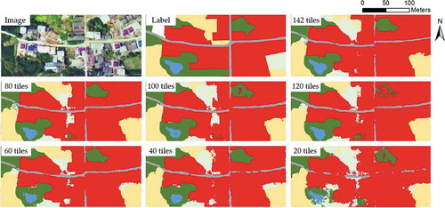
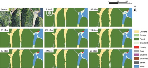
For the rural area where mainly consists of Forest, Cropland, and Water, however, the eroded-like boundary is not a notable problem (Figure 12). These classes have homogeneous textures and naturally curved boundaries. Both SegNet and U-Net return smooth boundaries in these areas, even trained with 40 tiles. The imbalance between urban and rural areas in our study area may cause different performances of DCNNs. The urban area takes up less than 10% in the experimental area, while the rural area covers more than 80%. In other words, the training samples of the urban area are only one-eighth of the samples in the rural area. We think the less training samples and the generalization of boundaries play a role in the relatively low performances of DCNNs in urban areas.

Figure 12. Land cover extraction results in a rural area. A small training set does not significantly decrease performances of DCNNs on boundaries of the land cover classes

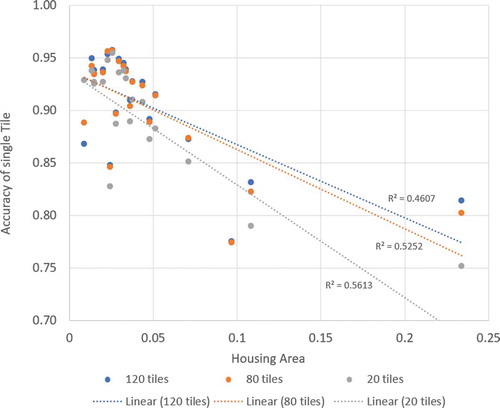
Figure 13 plots the performance of SegNet on each tile in the test set, and the model was trained by 120, 80, and 20 tiles, respectively. Usually, urban areas have more Housing Areas, so that we use the percentage of Housing Area to indicate the urbanization level. Figure 13 shows that when trained by smaller training sets, the model performance decreases more rapidly in urban areas.

Figure 13. When trained by smaller training sets, model performance decreases more rapidly in urban areas where contains more Housing Area.

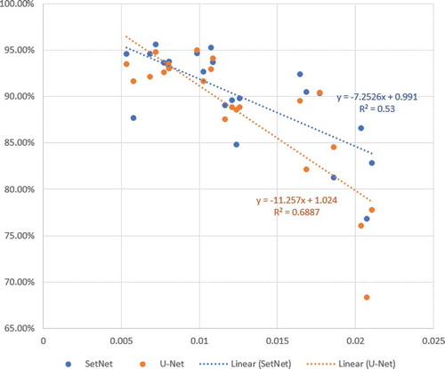
As mentioned by Heydari and Mountrakis (2018), the number of pixels on edges, or Edge-ratio, affects accuracy. In our case, when plotting the Edge-ratio and accuracy (from the training set of 120 tiles) of each tile in the test set (Figure 14), a decreasing trend was identified. A higher Edge-ratio leads a lower accuracy. This characteristic can be used for accuracy estimation and quality control in applications.

Figure 14. The relationship between Edge-ratio (x-axis) and accuracy (y-axis)

Segmentation results from larger training sets have better boundaries in this research. Other approaches are also available to improve the boundary representation, such as Conational Random Fields (CRF) (Panboonyuen et al. 2017; Fu et al. 2017) and morphological operation. We used open operations (10 × 10 pixels) and majority filter (3 × 3 pixels) respectively to smoothen the boundaries of the results of SegNet. These smoothing filters were applied to the segmentation results and the test set. The accuracies of the smoothed results slightly decrease (0.00006 and 0.00290), while the Edge-ratios (0.0112 and 0.0116) are close to the ground truth (0.0119). Thus, the boundary can be largely improved by appropriate post-processes with accuracy not affected. Edge-ratio is also useful to evaluate the effects of post-processes on the boundary.

Another insight from this study is to provide guidelines on how to apply DCNNs in practical segmentation projects. If a county needs a high-resolution land cover map for land resource management, the production team can manually label a small portion of the entire area, and then train a DCNN to finish the rest. We used the trained SegNet from a training set of 80 tiles to classify the remaining 62 tiles, obtaining an accuracy of 0.906, which is similar to the test set (26 tiles, 0.903). In our case, the rural area can get an acceptable accuracy of about 0.9, and the class boundary aligns well to the land cover class. In the urban area, DCNN does not show the capability to depict the boundary as a human annotator, but we suggest using DCNN to check whether or not the class of a manually drawn polygon is given correctly, rather than to delineate the class boundary.

Different strategies may affect the performance of DCNN. For instance, Rehman et al. (2018) used a modified resilient backpropagation algorithm to accelerate the convergence of CNN training. Caliskan et al. (2018) proposed a division of internal parameter space of DNN then optimize the small partitions individually. However, our paper focuses on the impact of the size of training sets on DCNN performance, and these same strategies may not be applicable. For example, data augmentation is necessary for small training sets, but not needful for large training sets, which have sufficient variance of samples.

Imbalanced class distribution is common among land covers on the Earth surface. Tackling an imbalanced training dataset is a hot research topic in machine learning. In a systematic study of the class imbalance problem on convolutional neural networks (Buda et al. 2018), the authors report that oversampling outperforms other alternatives in experiments. If applying oversampling to land cover research, a simple method is to duplicate the tiles with a large proportion of categories whose percentage is less in the total training set. For instance, Housing Area takes up about 5% in the study area and duplicating the tiles in urban and residential areas can increase its ratio in the training dataset.

For multi-class land cover applications (10 classes in our case), converting them to single class models using one-vs-rest or one-vs-one strategy will lead to explosions on numbers of binary models or datasets when the number of classes increases (Li et al. 2020; Di et al. 2019; Chen et al. 2016). Considering these strategies complicates the comparison between large and small training sets. To keep our converting guidelines relatively practical and straightforward, we do not go further to develop strategies on how to improve model performance.

In the future, more research are needed to better guide the conversion of land cover data to training sets. The first potential research is quantifying the relationship between the training set and the number of learnable parameters of DCNNs. SegNet used in this research has about 30 million parameters. The training set of 20 tiles includes 5 × 10⁹ pixels, which is 17 times as the number of parameters; it can train the SegNet in relatively high accuracy (0.8852). Meanwhile, U-Net has about 2 × 10⁷ parameters, and its performance is largely behind SegNet. The homogeneity and heterogeneity of the land cover data call for the necessity of investigating the quantitative relationship between the number of model parameters and the size of the training set. In addition, the impact of the imbalance of class distribution and the fine-grained segmentation are two important topics for DCNN-based land cover applications.

6. Conclusion

This study presents a viewpoint that existing land cover data is a potential training dataset for deep learning applications. This reuse of historical data is a valuable counterview that the inadequacy of training dataset challenges the deep learning research in remote sensing community (Ball, Anderson, and Chan 2017; Ball, Anderson, and Wei 2018). However, in practice, how to choose an appropriate size of training dataset when reusing existing data needs to be carefully considered to balance accuracy requirement and the computing time and resources. Using a county-level land cover dataset, we quantitatively explored the impact of the size of training sets using two popular architectures of DCNN for image semantic segmentation (SegNet and U-Net) when converting land cover data to training sets. Through the experiments, we document the relationship between the segmentation accuracy and the size of the training set, as well as the nonstationary accuracies among different land cover types as summarized below.

• In the rural area, where less infrastructure exists, DCNN needs fewer data to learn the features and can get better performance on class detection and boundary depiction.

• In an imbalanced training set, classes with limited coverage of the study area often have poor accuracies. Data augmentation and training tuning may be needed to improve the performance of DCNN.

• Deep learning techniques are not suitable for certain applications in land cover segmentation. Some land cover classes in this research, such as Structure, Excavated land, Grass, and Orchard, trend to be misclassified as other classes with similar textures in 0.5 m RS images.

• The new Edge-ratio metrics can be used to evaluate the segmentation results. The result with an Edge-ratio closer to the ground truth has a better representation of the class boundaries.

n the remote sensing field, we still lack methods and guidelines to efficiently reuse the massive historical high-quality data. Findings of this paper offer valuable insights on effectively tailoring the existing land cover data to training sets, and thus accelerate the assessment and employment of deep learning techniques for high-resolution land cover map extraction and other deep learning-assisted approaches.

Disclosure statement

No potential conflict of interest was reported by the authors.

References

- Audebert, N., B. Le Saux, and S. Lefevre. 2017. “Joint Learning from Earth Observation and OpenStreetMap Data to Get Faster Better Semantic Maps.” 67–75. http://openaccess.thecvf.com/content_cvpr_2017_workshops/w18/html/Audebert_Joint_Learning_From_CVPR_2017_paper.html
- Audebert, N., B. Le Saux, and S. Lefèvre. 2018. “Beyond RGB: Very High Resolution Urban Remote Sensing with Multimodal Deep Networks.” ISPRS Journal of Photogrammetry and Remote Sensing, Geospatial Computer Vision 140 (June): 20–32. doi:https://doi.org/10.1016/j.isprsjprs.2017.11.011.
- Badrinarayanan, V., A. Kendall, and R. Cipolla. 2017. “SegNet: A Deep Convolutional Encoder-Decoder Architecture for Image Segmentation.” IEEE Transactions on Pattern Analysis and Machine Intelligence 39 (12): 2481–2495. doi:https://doi.org/10.1109/TPAMI.2016.2644615.
- Ball, J. E., D. T. Anderson, and C. S. Chan. 2017. “Comprehensive Survey of Deep Learning in Remote Sensing: Theories, Tools, and Challenges for the Community.” Journal of Applied Remote Sensing 11 (4): 042609. doi:https://doi.org/10.1117/1.JRS.11.042609.
- Ball, J. E., D. T. Anderson, and P. Wei. 2018. “State-of-the-Art and Gaps for Deep Learning on Limited Training Data in Remote Sensing.” ArXiv Preprint. ArXiv:1807.11573.
- Buda, M., Maki, A., & Mazurowski, M. A. (2018). A systematic study of the class imbalance problem in convolutional neural networks. Neural Networks, 106, 249-259. doi:https://doi.org/10.1016/j.neunet.2018.07.011
- Caliskan, A., M. E. Yuksel, H. Badem, and A. Basturk. 2018. “Performance Improvement of Deep Neural Network Classifiers by a Simple Training Strategy.” Engineering Applications of Artificial Intelligence 67 (January): 14–23. doi:https://doi.org/10.1016/j.engappai.2017.09.002.
- Chen, J., L. Wu, K. Audhkhasi, B. Kingsbury, and B. Ramabhadrari. 2016. “Efficient One-vs-One Kernel Ridge Regression for Speech Recognition.” In 2016 IEEE International Conference on Acoustics, Speech and Signal Processing (ICASSP), 2454–2458. doi:https://doi.org/10.1109/ICASSP.2016.7472118.
- Dai, D., and W. Yang. 2011. “Satellite Image Classification via Two-Layer Sparse Coding with Biased Image Representation.” IEEE Geoscience and Remote Sensing Letters 8 (1): 173–176. doi:https://doi.org/10.1109/LGRS.2010.2055033.
- Di, Z., Q. Kang, D. Peng, and M. Zhou. 2019. “Density Peak-Based Pre-Clustering Support Vector Machine for Multi-Class Imbalanced Classification.” In 2019 IEEE International Conference on Systems, Man and Cybernetics (SMC), 27–32. doi:https://doi.org/10.1109/SMC.2019.8914451.
- Fonte, C. C., Minghini, M., Patriarca, J., Antoniou, V., See, L., & Skopeliti, A. (2017). Generating up-to-date and detailed land use and land cover maps using OpenStreetMap and GlobeLand30. ISPRS International Journal of Geo-Information, 6(4), 125. doi:https://doi.org/10.3390/ijgi6040125
- Fu, G., C. Liu, R. Zhou, T. Sun, and Q. Zhang. 2017. “Classification for High Resolution Remote Sensing Imagery Using a Fully Convolutional Network.” Remote Sensing 9 (5): 498. doi:https://doi.org/10.3390/rs9050498.
- Ghaffarian, S., N. Kerle, E. Pasolli, and J. J. Arsanjani. 2019. “Post-Disaster Building Database Updating Using Automated Deep Learning: An Integration of Pre-Disaster OpenStreetMap and Multi-Temporal Satellite Data.” Remote Sensing 11 (20): 2427. doi:https://doi.org/10.3390/rs11202427.
- Goodfellow, I., J. Pouget-Abadie, M. Mirza, B. Xu, D. Warde-Farley, S. Ozair, A. Courville, and Y. Bengio. 2014. “Generative Adversarial Nets.” In Z. Ghahramani and M. Welling and C. Cortes and N.D. Lawrence and K.Q. Weinberger (Eds.)., Advances in Neural Information Processing Systems, 2672–2680. https://papers.nips.cc/book/advances-in-neural-information-processing-systems-27-2014
- Grippa, T., S. Georganos, S. Zarougui, P. Bognounou, E. Diboulo, Y. Forget, M. Lennert, S. Vanhuysse, N. Mboga, and E. Wolff. 2018. “Mapping Urban Land Use at Street Block Level Using OpenStreetMap, Remote Sensing Data, and Spatial Metrics.” ISPRS International Journal of Geo-Information 7 (7): 246. doi:https://doi.org/10.3390/ijgi7070246.
- Haklay, M., and P. Weber. 2008. “Openstreetmap: User-Generated Street Maps.” IEEE Pervasive Computing 7 (4): 12–18. doi:https://doi.org/10.1109/MPRV.2008.80.
- Heydari, S. S., and G. Mountrakis. 2018. “Effect of Classifier Selection, Reference Sample Size, Reference Class Distribution and Scene Heterogeneity in per-Pixel Classification Accuracy Using 26 Landsat Sites.” Remote Sensing of Environment 204 (January): 648–658. doi:https://doi.org/10.1016/j.rse.2017.09.035.
- Huang, B., B. Zhao, and Y. Song. 2018. “Urban Land-Use Mapping Using a Deep Convolutional Neural Network with High Spatial Resolution Multispectral Remote Sensing Imagery.” Remote Sensing of Environment 214 (September): 73–86. doi:https://doi.org/10.1016/j.rse.2018.04.050.
- Ioffe, S., and C. Szegedy. 2015. “Batch Normalization: Accelerating Deep Network Training by Reducing Internal Covariate Shift.” ArXiv:1502.03167 [Cs], February. http://arxiv.org/abs/1502.03167
- I.owa Department of Natural Resources. 2009. “LandCover/LC_2009_1m (MapServer).” Iowa Department of Natural Resources. https://programs.iowadnr.gov/geospatial/rest/services/LandCover/LC_2009_1m/MapServer
- Jin, H., S. V. Stehman, and G. Mountrakis. 2014. “Assessing the Impact of Training Sample Selection on Accuracy of an Urban Classification: A Case Study in Denver, Colorado.” International Journal of Remote Sensing 35 (6): 2067–2081. doi:https://doi.org/10.1080/01431161.2014.885152.
- Längkvist, M., A. Kiselev, M. Alirezaie, and A. Loutfi. 2016. “Classification and Segmentation of Satellite Orthoimagery Using Convolutional Neural Networks.” Remote Sensing 8 (4): 329. doi:https://doi.org/10.3390/rs8040329.
- Li, N., H. Hao, Z. Jiang, F. Jiang, R. Guo, G. Qing, and X. Hu. 2020. “A Multi-Task Multi-Class Learning Method for Automatic Identification of Heavy Minerals from River Sand.” Computers & Geosciences 135 (February): 104403. doi:https://doi.org/10.1016/j.cageo.2019.104403.
- Lin, T.-Y., M. Maire, S. Belongie, J. Hays, P. Perona, D. Ramanan, P. Dollár, and C. Lawrence Zitnick. 2014. “Microsoft COCO: Common Objects in Context.” In Computer Vision – ECCV 2014, 740–755. Lecture Notes in Computer Science. Cham: Springer. doi:https://doi.org/10.1007/978-3-319-10602-1_48.
- Liu, W., Z. Wang, X. Liu, N. Zeng, Y. Liu, and F. E. Alsaadi. 2017. “A Survey of Deep Neural Network Architectures and Their Applications.” Neurocomputing 234 (April): 11–26. doi:https://doi.org/10.1016/j.neucom.2016.12.038.
- Long, J., E. Shelhamer, and T. Darrell. 2015. “Fully Convolutional Networks for Semantic Segmentation.” 3431–3440. https://www.cv-foundation.org/openaccess/content_cvpr_2015/html/Long_Fully_Convolutional_Networks_2015_CVPR_paper.html
- Luo, N., T. Wan, H. Hao, and Q. Lu. 2019. “Fusing High-Spatial-Resolution Remotely Sensed Imagery and OpenStreetMap Data for Land Cover Classification over Urban Areas.” Remote Sensing 11 (1): 88. doi:https://doi.org/10.3390/rs11010088.
- Ma, L., M. Li, X. Ma, L. Cheng, P. Du, and Y. Liu. 2017. “A Review of Supervised Object-Based Land-Cover Image Classification.” ISPRS Journal of Photogrammetry and Remote Sensing 130 (August): 277–293. doi:https://doi.org/10.1016/j.isprsjprs.2017.06.001.
- Ma, L., Y. Liu, X. Zhang, Y. Ye, G. Yin, and B. A. Johnson. 2019. “Deep Learning in Remote Sensing Applications: A Meta-Analysis and Review.” ISPRS Journal of Photogrammetry and Remote Sensing 152 (June): 166–177. doi:https://doi.org/10.1016/j.isprsjprs.2019.04.015.
- McCann, M. T., K. H. Jin, and M. Unser. 2017. “A Review of Convolutional Neural Networks for Inverse Problems in Imaging.” IEEE Signal Processing Magazine 34 (6): 85–95. doi:https://doi.org/10.1109/MSP.2017.2739299.
- Panboonyuen, T., K. Jitkajornwanich, S. Lawawirojwong, P. Srestasathiern, and P. Vateekul. 2017. “Road Segmentation of Remotely-Sensed Images Using Deep Convolutional Neural Networks with Landscape Metrics and Conditional Random Fields.” Remote Sensing 9 (7): 680. doi:https://doi.org/10.3390/rs9070680.
- Rehman, S. U., T. Shanshan, O. U. Rehman, H. Yongfeng, C. M. Sarathchandra Magurawalage, and C.-C. Chang. 2018. “Optimization of CNN through Novel Training Strategy for Visual Classification Problems.” Entropy 20 (4): 290. doi:https://doi.org/10.3390/e20040290.
- Ronneberger, O., P. Fischer, and T. Brox. 2015. “U-Net: Convolutional Networks for Biomedical Image Segmentation.” In International Conference on Medical Image Computing and Computer-Assisted Intervention, 234–241. Munich, Germany: Springer.
- Rottensteiner, F., G. Sohn, J. Jung, M. Gerke, C. Baillard, S. Benitez, and U. Breitkopf. 2012. “The ISPRS Benchmark on Urban Object Classification and 3D Building Reconstruction.” The ISPRS Annals of the Photogrammetry, Remote Sensing and Spatial Information Sciences 1 (3): 293–298. doi:https://doi.org/10.5194/isprsannals-I-3-293-2012.
- Russakovsky, O., J. Deng, S. Hao, J. Krause, S. Satheesh, S. Ma, Z. Huang, et al. 2015. “ImageNet Large Scale Visual Recognition Challenge.” International Journal of Computer Vision 115 (3): 211–252. doi:https://doi.org/10.1007/s11263-015-0816-y.
- Scott, G. J., R. A. Marcum, C. H. Davis, and T. W. Nivin. 2017. “Fusion of Deep Convolutional Neural Networks for Land Cover Classification of High-Resolution Imagery.” IEEE Geoscience and Remote Sensing Letters 14 (9): 1638–1642. doi:https://doi.org/10.1109/LGRS.2017.2722988.
- Sherrah, J. 2016. “Fully Convolutional Networks for Dense Semantic Labelling of High-Resolution Aerial Imagery.” ArXiv:1606.02585 [Cs], June. http://arxiv.org/abs/1606.02585
- Xinhua. 2017. “China Unveils Results of First Geoinformation Survey.” People’s Daily Online. People’s Daily Online. April 25. http://en.people.cn/n3/2017/0425/c90000-9207010.html
- Yang, Y., and S. Newsam. 2010. “Bag-of-Visual-Words and Spatial Extensions for Land-Use Classification.” In Proceedings of the 18th SIGSPATIAL International Conference on Advances in Geographic Information Systems, 270–279. GIS ’10. New York, NY: ACM. doi:https://doi.org/10.1145/1869790.1869829.
- Zeiler, M. D., and R. Fergus. 2014. “Visualizing and Understanding Convolutional Networks.” In Computer Vision – ECCV 2014, edited by D. Fleet, T. Pajdla, B. Schiele, and T. Tuytelaars, 818–33.Lecture Notes in Computer Science. Zurich, Switzerland: Springer International Publishing. https://link.springer.com/book/10.1007/978-3-319-10590-1
- Zhang, C., I. Sargent, X. Pan, H. Li, A. Gardiner, J. Hare, and P. M. Atkinson. 2018. “An Object-Based Convolutional Neural Network (OCNN) for Urban Land Use Classification.” Remote Sensing of Environment 216: 57–70. doi:https://doi.org/10.1016/j.rse.2018.06.034.
- Zhao, W., Y. Bo, J. Chen, D. Tiede, T. Blaschke, and W. J. Emery. 2019. “Exploring Semantic Elements for Urban Scene Recognition: Deep Integration of High-Resolution Imagery and OpenStreetMap (OSM).” ISPRS Journal of Photogrammetry and Remote Sensing 151 (May): 237–250. doi:https://doi.org/10.1016/j.isprsjprs.2019.03.019.
- Zhen, Z., L. J. Quackenbush, S. V. Stehman, and L. Zhang. 2013. “Impact of Training and Validation Sample Selection on Classification Accuracy and Accuracy Assessment When Using Reference Polygons in Object-Based Classification.” International Journal of Remote Sensing 34 (19): 6914–6930. doi:https://doi.org/10.1080/01431161.2013.810822.
- Zhu, X., C. Vondrick, C. C. Fowlkes, and D. Ramanan. 2016. “Do We Need More Training Data?” International Journal of Computer Vision 119 (1): 76–92. doi:https://doi.org/10.1007/s11263-015-0812-2.
- Zhu, X. X., D. Tuia, L. Mou, G.-S. Xia, L. Zhang, F. Xu, and F. Fraundorfer. 2017. “Deep Learning in Remote Sensing: A Review.” IEEE Geoscience and Remote Sensing Magazine 5 (4): 8–36. doi:https://doi.org/10.1109/MGRS.2017.2762307.