Spatial search and a three level model based water layer extraction from C-band SAR image

ABSTRACT

This paper describes a spatial search and a three-level model-based approach for automatic extraction of surface water layers from Sentinel-1 C-band SAR images at 10 m spatial resolution. The technique incorporates a connected component spatial search for segmenting low backscatter regions and uses the segmented image object for characterizing the segments. The water body is described here as a collection of different spatially connected segments. A three-level model is used to describe the connected segments of a water body in SAR data. Noise tolerance is achieved in this method by incorporating a speckle noise level into the model. The segmentation process further calculates contextual information which includes shadow estimated from DEM, polarization angle of the segment, and a boundary co-occurrence in both polarization to qualify the detected segments as a water body. The proposed method is found to have an accuracy of 94% in terms of f1 score. The algorithm, estimation of different parameters, and the results obtained in selected regions are explained in this paper.

KEYWORDS:

• SAR
• ann
• obia
• water body
• feature extraction
• microwave remote sensing

1. Introduction

Information regarding surface water is a very significant parameter in resource planning. Estimation, monitoring, and conservation of water bodies are essential for human development. Water bodies are more dynamic and experience large wastage as surface run-off during rainy season often affecting transport lines and community hygiene. Information regarding spatially and temporally dynamic water bodies is essential for water resource management, planning and hydrology studies.

Clouds often make the observation from space using optical sensors obscure mainly during the rainy season. Since SAR is an active mode of remote sensing and is least affected by cloud and illumination, water body estimation from SAR data is essential for hydrology studies. To find sporadic water bodies, the algorithm must be constrained to detect all significant water bodies independent of its past occurrences.

Delineation of sea ice and open water from dual pol SAR images using decision tree is described in (Geldsetzer and Yackel 2009). The different thresholds for the decision tree are estimated statistically from the Horizontal and Vertical polarized data and their ratio. Methods using Active contours used to delineate water bodies from land are described in (Silveira and Heleno 2008, 2009). Region-based methods require an initial region to be defined manually over the area of interest which makes automatic detection of water bodies difficult. Monitoring of surface water with Neural Network is described in (Pham-Duc, Prigent, and Aires 2017). Most of the feature extraction algorithms for SAR data employ a de-speckling filter which reduces the effect of speckle noise on the image preserving essential features (Lee et al. 2009; Lee 1983; Wang and Li 2015). The performance of widely used de-speckling filters is analysed in (Anand, Marappan, and Sethumadhavan 2018; Sun et al. 2016). In the proposed methodology. The requirement of a speckle filter is avoided by incorporating speckle as part of the SAR water model.

Object Based Image Analysis (OBIA) brought in a paradigm shift from pixel to segment-based image processing (Blaschke 2010). It is extensively used in many remote sensing applications, mostly in multispectral, hyper spectral and thermal remote sensing (Bechtel, Ringeler, and Bohner 2008). Region Growing algorithms are widely used for image segmentation. These methods segment images based on a similarity condition to properly find the boundary between two segments. These algorithms are tailored to work under varying lighting conditions, which is common in optical images.

Unlike optical sensors, a SAR sensor always looks at the scene in the off-nadir direction. This imaging geometry results in geometric and radiometric distortions like foreshortening, layover, shadow etc caused by the topographical variations in a scene. SAR being an active mode of remote sensing, the sensitivity of the image formed varies across the scene due to the gain variation of the antenna system (Loew and Mauser 2007). Radar backscatter from the target is a function of its dielectric constant, orientation (incidence angle), shape and distribution. For a distributed target like the surface of the earth, it is the coherent summation of backscatter from each target added with noise. For a target like water body, the backscattered power can be considered as the sum of noise and low backscatter due to specular reflection over the calm area and coherent summation of scattering from waves on the surface of the water. Speckle noise is characteristic of SAR data due to the limited bandwidth and coherent imaging technique. Speckle by its nature is random and uniformly distributed in space. A detailed study of speckle and its properties was carried out using laser speckle (Goodman 1975).

Speckle noise is found to be dependent on system parameters like aperture size, shape and bandwidth of the electromagnetic wave (Zhang and Zhensen 2010). In SBIA the speckle power is estimated from its spatial characteristics and used to refine the three-level water body model parameters. The effect of speckle is reduced by detecting it and merging it with the segmented water layer. The speckle is detected in the water region by defining a speckle level and initiating an area limited search on connected speckle level (section 2.3). This avoids the need for filtering the data with de-speckling filters, and its spatial spread is used to effectively coalesce the fragmented segments.

Radar being an active mode of imaging, data are having minimal effect on extraneous factors like sun illumination and atmospheric conditions. This property of SAR images allows us to reliably explore the data with fixed or predictable thresholds. In this paper, we propose a new approach where the segmentation algorithm is aware of speckle and is part of the water body model. The algorithm is inspired by region growing technique, where the segmented region grows from a seed point adding connected neighbours to the segments. Instead of a dynamically estimated similarity condition, the membership functions are based on pre-estimated intensity levels.

At microwave frequencies, the backscattered power from a target is characteristic of its surface roughness and the dielectric constant. Due to high dielectric constant, low surface roughness, and imaging geometry, water bodies appear as dark (low backscatter) regions in C-band SAR images. The proposed SBIA uses a multilevel search along with a three-level model for the water body to segment neighbour connected low backscatter region, taking into account the radiometric and spatial spread of speckle. The method avoids the use of any spatial or temporal filtering and it uses the speckle noise to estimate water model parameters. It uses a combined OBIA and an expert system for better noise immunity and class separability. SBIA detects all possible candidates for a water body and eliminates those segments which do not qualify for water body inferred from observations of the segmented pixels and its context.

An expert system-based mapping and study of long-term changes in surface water at a global scale for 35 years at 30 m resolution from Landsat satellite images is explained in (Pekel et al. 2016). The system provides various parameters for the long-term dynamics of water bodies. SBIA is validated against the Global water layer for comparable water bodies. Segmentation accuracy is estimated using manually digitized water body from optical satellite imagery.

This paper is organized as follows. SBIA algorithm, the three-level model for a water body, and parameter estimation for the proposed method is described in section 2. Details about the data used are explained in 3. Details about the implementation of Sentinel-1 data are explained in section 4. The results and validation of the algorithm are discussed in section 5.

2. Search-based image analysis

A search is an iterative algorithm to collect all points which are connected by a neighbour (Section 2.1). The search is supplemented with a boolean membership function with which it collects all connected pixels satisfying the boolean membership condition. Due to speckle noise and other disturbances in water bodies, it is practically difficult to reliably segment the entire water body region with a single search. The water body is split into different connected segments with a three-level model as described in section 2.3. The different considerations and analysis used in estimating constraints for the three levels are described in section 2.4 A multilevel search iteratively collects results from spatially connected searches using different membership conditions. The segments collected using multilevel search are combined based on conditions described in section 2.5.

2.1. Search by levels

A search starts from a seed point and propagates to its neighbours recursively with a Boolean membership function $M_{li}(x)$ on a radiometric interval $l_i$. The search algorithm produces two lists of pixels. One list that satisfies $M_{li}(x)$ and which don’t satisfy in the neighbour connected region as result list and neighbour list respectively. For a scene $S$, with starting point $p_0$ and radiometric interval $l_i$ the search algorithm can be expressed in a pseudo-code as follows.

procedure Search($S,l_i,p_0$) ▹Search $S$ for $l_i$ at $p_0$

Work list$\leftarrow \{p_0\}$ ▹Initialize Work list with seed point

Result list$\leftarrow \varphi$ ▹Initialize result with empty list ($\varphi$)

Neighbour list$\leftarrow \varphi$ ▹Initialize variables with empty list

History$\leftarrow \varphi$

while Work list$\ne \varphi$ do

POP(Work list)

if $p_t\notin$ History then

if $M_{li}(p_t)=1$ then

PUSH(Result List,$p_t$)

Neighbours = $N_S(p_t)$▹Get neighbours

APPEND(Work list, Neighbours)

else

PUSH(Neighbour list, $p_t$)

end if

PUSH(History, $p_t$)

end if

end while

return Result List, Neighbour list

end procedure

Parameters like the area of the region and distribution of its context are derived from the result list and neighbour list provided by the search algorithm.

2.2. Searching with multiple levels

A search with single interval $l_i$ will give connected region satisfying the membership condition $M_{li}(x)$. Noise makes the whole region fragmented making it impossible for a single search to cover the whole region. In order to address this, the search is extended to more levels as explained in section 2.3. The segments at each level are merged as explained in section 2.5. The search is conducted on a contiguous set of disjoined intervals $\mathbb{L}$ (equation 1(1) $\mathbb{L}=\{[0,l_0),[l_0,l_1),[l_1,l_2)..[l_{n-1},l_n)\}$(1) ). The interval boundaries are represented by a level boundary list $L$ (equation 2(2) $L=\{l_0,l_1,l_2,\dots l_n\}$(2) ). The boolean membership condition for a given radiometric value $x$ is given by a relational operation as in equation 3(3) $M_{li}(x)=\left\{\begin{array}{cc}1,& \mathrm{f}\mathrm{o}\mathrm{r}{l}_{i-1}\le x<l_i\\ 0,& \mathrm{f}\mathrm{o}\mathrm{r}\mathrm{o}\mathrm{t}\mathrm{h}\mathrm{e}\mathrm{r}\mathrm{s}\end{array}\right.$(3) . The interval boundary index can be estimated as in equation 4(4) $L(x)=\underset{{ }_{l_i\in L}}{argmin}(M_{li}(x))$(4) .

(1) $\mathbb{L}=\{[0,l_0),[l_0,l_1),[l_1,l_2)..[l_{n-1},l_n)\}$(1)

(2) $L=\{l_0,l_1,l_2,\dots l_n\}$(2)

(3) $M_{li}(x)=\left\{\begin{array}{cc}1,& \mathrm{f}\mathrm{o}\mathrm{r}{l}_{i-1}\le x<l_i\\ 0,& \mathrm{f}\mathrm{o}\mathrm{r}\mathrm{o}\mathrm{t}\mathrm{h}\mathrm{e}\mathrm{r}\mathrm{s}\end{array}\right.$(3)

(4) $L(x)=\underset{{ }_{l_i\in L}}{argmin}(M_{li}(x))$(4)

Where $L(x)$ in the level index of a scalar backscatter value $x$. The neighbours of point $p_{x,y}$ at coordinate $(x,y)$ in a scene $S$ is given by

(5) $N_S(p)=\{q\subseteq {\mathbb{R}}^2:L_{\mathrm{\infty }}(p,q)=1andq\in S\}$(5)

Where $L_{\mathrm{\infty }}$ is the Chebyshev distance or maximum metric (Cantrell 2000) given as the greatest of difference along any coordinate dimension (Abello, Pardalos, and Resende 2013)

(6) $L_{\mathrm{\infty }}(p,q)=\underset{i\in \{x,y\}}{max}(|p_i-q_i|)$(6)

Children for a single iteration in search are given by equation 7(7) $Ch(p)=\{x\in N(p):L(p)=L(x)\}$(7) and the excluded neighbour list is given by equation 8(8) $Neigh(p)=\{x\in N(p):L(p)\ne L(x)\}$(8) .

(7) $Ch(p)=\{x\in N(p):L(p)=L(x)\}$(7)

(8) $Neigh(p)=\{x\in N(p):L(p)\ne L(x)\}$(8)

A recursive Neighbourhood search with $M_{li}$ as the search criteria at $p_1$ collect all points which have neighbourhood connectivity and support for the parent level. A search gives two lists, a segmented region belonging to the current level and a list of adjacent points which do not belong to the current level but are connected to the current segment (neighbours). The algorithm for multiple-level search can be described as

1. procedure M-Search ($S,p_0$) M-Search $S$ at $p_0$

2. Work list$\leftarrow \{p_0\}$ Initialize Work list with seed point

3. Result list$\leftarrow \varphi$ Initialize result with empty list

4. while Work list $\ne \varphi$ do

5. $p_1\leftarrow$POP(Work list)

6. neighbours, result$\leftarrow$ Search($S,li,p_1$)

7. APPEND(Work list, neighbours)

8. PUSH(Result list, (neighbours, result))

9. end while

10. return Result list

11. end procedure

M-Search gives result and neighbour lists corresponding to each connected segment found in the region.

2.3. Three level model for water in SAR images

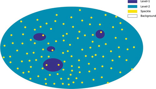
To describe the water body in the search paradigm and to estimate different parameters for the search algorithm, a model for a water body in SAR data is devised. A water body in SAR image can be represented spatially by the model as shown in Figure 1. The model consists of segments belonging to three levels which can be delineated using level-based search. The levels and their significance are described as follows.

• Level 1 a low backscatter region which is radiometrically disjointed with background. This level acts as the seed point for initiating the search.

• Level 2 low backscatter regions which have radiometric overlap and spatially disjointed with background. This level is expected to cover the major part of the water body.

• Level 3 (speckle) High backscatter speckle level with numerous and spatially small segments. This level is essential to connect the fragmented level 2 segments.

Figure 1. Three Level model for water body

2.4. Level design

The levels were designed by studying the nature and spread of the search over known regions at different incident angles. For this study, various AOIs were manually drawn around different water bodies. The distribution of the AOIs in the image is shown in figs 4b and 4a. Figures 2 show three AOIs among 27 water bodies chosen for the study.

Figure 2. Input image with manually drawn AOI, normalized histogram of pixels inside AOI, outside AOI, total image and the normalized variation of number of segments in level 2 and level 3 at with level 2-3 boundary in the corresponding AOIs

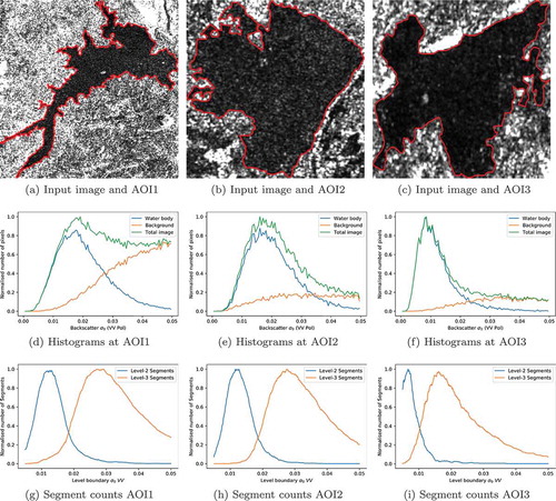
Figure 3. Three level segmentation for a selected AOI using SBIA showing speckle level extending into non-water regions (Area: Hyderabad, India. DOP:8 October 2018)

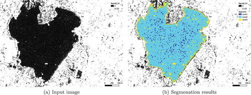
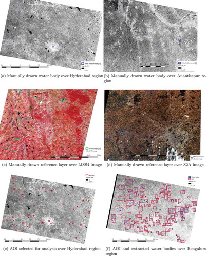
Figure 4. Manually drawn AOI and reference layers for analysis

2.4.1. Level 1 seed point level

Since the search algorithm starts with this level. For reliable detection of all water bodies, every water body in a scene should contain at least one segment with this level. For estimating the level 1 boundaries, many water bodies are manually selected from different regions of the data set. AOI is drawn over selected water bodies and histogram of pixels is calculated inside and outside the water body and the total rectangular AOI. The histograms for three selected water bodies are shown in Figure 2. Level boundary $l_0$ is estimated from the histograms as the minimum of all pixel levels in the selected AOIs. $l_1$ is estimated as the minimum of the histogram where the total histogram is equal to the histogram of AOI and satisfying the condition in equation 9(9) $l_1\ge \underset{i=0}{\overset{n}{max}}(\underset{j=0}{\overset{s_i}{min}}(p_{ij}))$(9) . In a region $R$ with $n$ water body and $s_i$ number of pixels in each water body $p_i$, $l_1$ should satisfy the minimum condition.

(9) $l_1\ge \underset{i=0}{\overset{n}{max}}(\underset{j=0}{\overset{s_i}{min}}(p_{ij}))$(9)

$\mathrm{\forall }{p}_{ij}\in R$

$l_1$ is practically chosen to a point where histograms of pixels inside water body are close (difference less than 1%) to histogram of the rectangular AOI. This gives a level which is disjoined with other pixels in the AOI.

2.4.2. Level 2 water segment level

This level is expected to segment the water body ideally into a single segment. The upper-level boundary of this level can be fixed by taking into account the properties of speckle noise. Speckles appear as randomly distributed small patterns. Value for $l_2$ is estimated by sweeping the $l_2$ and conducting search in with the modified $l_2$. Figures 2 give the variation of number of segments in $L_2$ and $L_3$ with $l_2$. The optimum value of $l_2$ is characterized by the maximum number of segments in the speckle level($L_3$) and minimum segments in the water segment level($L_2$). $l_2$ is fixed to mean of all $l_2$ yielding maximum segments in $L_3$.

2.4.3. Level 3 speckle level

The function of this segment is to bridge two separated water segments due to the effect of speckle and other noises. This level is estimated with water bodies having high backscatter due to waves and low incidence angle. Level boundary $l_3$ is fixed to the maximum of backscatter in selected AOIs. The level is searched with an area constraint which is estimated from the spread of speckle in the selected AOIs. Segments and children of level 3 search having area greater than the estimated constraint are discarded from the result.

2.5. Merging of segments

The different segments collected by a multilevel search are combined to form a single segment. Level-2 segments which are collected which have Level 1 segment as parent or have Level 1 segments as neighbours are combined. As Level 3 in the model is expected to segment only the speckle which is characterized by small spatial spread. Level 3 segments and segments which are children of a Level 3 search are combined with constraints.

2.5.1. Area constrains

The speckle level (Level 3) segments are characterized by small area per segment and have large radiometric overlap with the background. In order to prevent background from merging into water segment, Level 3 searches are combined with an area constraint. The number of pixels that can be considered is estimated from the distribution of segment size in $l_2$ parameter sweep explained in Sec. 2.4.2. Area constraint is fixed to a value that is grater than the majority of segment size of segments in $L_3$ level at the point where number of segments in $L_3$ is high. For segments having size greater than the area constraint, the segment and its children collected are discarded from results and further searches.

2.5.2 . Conditions based on neighbours

At the boundary of water bodies, speckle levels tend to include non-water pixels into water segment. The segmented image using search is shown in Figure 3. In order to eliminate this effect, the segments were merged using an expert system based on levels of the neighbours. For each segment, level of the region($l_r$), minimum of level among neighbours($n_{min}$) and maximum of level among neighbours($n_{max}$) are estimated as.

(10) $R,N\leftarrow M-Search(S,p_0)$(10)

(11) $l_r=L(r)\mathrm{\forall }r\in R$(11)

(12) $n_{min}=\underset{i}{min}(L(N_{ei}))$(12)

(13) $n_{max}=\underset{i}{max}(L(N_{ei}))$(13)

Where $min$ and $max$ are minimum and maximum respectively. For a region having $n$ subregions, a logical rule on these observations is used to merge the sections to form a single region.

(14) $R_w=\underset{i=1}{\overset{n}{\cup }}{R}_i:\begin{array}{c}{l}_r=1,\hspace{0.17em}\\ l_r=2\\ l_r=3\end{array}\hspace{0.17em}\begin{array}{c}\hspace{0.17em}\\ n_{min}=1,\\ n_{max}\le 2\end{array}\hspace{0.17em}$(14)

The water segments $R_w$ are combined to form the water region.

3. Data and study area

Region between Hyderabad and Bangalore which covers three states viz Telangana, Andhra Pradesh and Karnataka were chosen for analysis. The area being part of the Deccan Plateau is less mountainous. Numerous water bodies in the form of reservoirs and tanks are the main water sources as the rivers are mostly non-perennial in nature. The data used is Sentinal-1A IW Level-1 Ground Range Detected (GRD) dual pol data at 10 m spatial resolution (ESA 2018). Date Of Pass (DOP), Location and number of water bodies selected from each dataset for analysis are summarized in Table 1. SRTM 1 Arc-Second DEM (NASA n.d.) was used for Range Doppler Terrain correction and shadow detection. LISS-IV (DOP:18 November 2017) and Sentinel-2A (DOP:23 November 2017) optical satellite images were used to manually generate the reference water layer for validating the algorithm. Figures 4 show the distribution of manually drawn reference layers over the corresponding optical image.

Table 1. Details of data used

Location	Date of Pass	Area analysed	Remark
77.506E,13.246 N	2017–11-18	1,290,119 ha	Bengaluru
77.773E,14.671 N	2017–11-18	150,501 ha	Anathapur
78.098E,16.278 N	2017–05-22	10,877 ha	Kurnool
78.429E,17.764 N	2018–01-05, 2018–02-10, 2018–03-06, 2018–04-11, 2018–05-05, 2018–06-22, 2018–07-04, 2018–08-09, 2018–09-02, 2018–10-08, 2018–11-01, 2018–12-07	53,139 ha/scene	Hyderabad

4. Methodology

Figure 5 gives the block diagram of the algorithm. The input data is calibrated, applied antenna and terrain correction using SNAP programme

Figure 5. Generalized Block diagram for Search Based Image Analysis

Figure 6. Distribution of mean magnitude and angle of polarization in water and non-water segments

provided by ESA (Section 4.1). Pre-processed image is then searched systematically (every pixel) for Level 1 points to start a search-based segmentation (section 4.2). In search-based segmentation instead of mapping each pixel, a cluster of locally connected pixels is grouped as a segment and is then processed by a rule-based expert system (section 2.5). Context information of the segment is also estimated in the process of segmentation from the neighbour pixels which were excluded from the segment. The expert system characterizes the segment based on secondary observations from the segment like shore support, Polarization, shadow and grazing angle (section 4.4.3). The estimated algorithm parameters for the given data are summarized in Table 2.

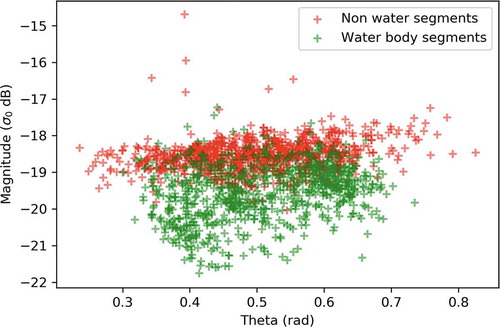
Table 2. Parameters used

parameter	value	remarks
level1	[0, 0.0071)	Estimated from histogram (Section 2.4.1)
level2	[0.005, 0.015)	Estimated from segment distribution (Section 2.4.2)
level3	[0.018, 0.4)	Estimated from speckle distribution (Section 2.4.3)
area constrain	10 pixels	Estimated from size of segments in level3 (Section 2.5.1)

4.1. Preprocessing

The SAR image is calibrated to backscattering coefficient (${\sigma }_0$) using calibration constants available in the metadata. Due to topographical variations on earth and the tilt of the satellite sensor, distances can be distorted in the SAR images. Terrain corrections compensate for these distortions so that the geometric representation of the image will be as close as possible to the real world. Calibrated and geocoded SAR image is converted into a geometrically corrected image by Range Doppler Terrain Correction operator available in SNAP tool, provided by ESA. It uses Range Doppler orthorectification method (Small and Schubert 2008). It uses available orbit state vector information in the metadata like radar timing annotations and slant to ground range conversion parameters together with SRTM DEM as reference DEM data to derive the precise geolocation information. The orthorectified image is geo-referenced to WGS-84 coordinate reference system so that each pixel can be mapped to the corresponding geographic coordinates.

4.2. Search Initialization (searching seed points)

First Step in the algorithm is to find the seed points where the search can be initialized. Seed points are collected by systematically searching the whole area of interest line by line. Systematic search gives seed points where it finds a low backscattered pixel (pixel value $<l_0$) as explained in section 2.4. A multilevel search is started at the seed point. Multilevel search (section 2.2) will segment all points which have connectivity to the seed point using the search. A search algorithm searches the image with discrete predefined intervals ($L$) as described in Section 2.4.

4.3. Boundary extraction

For the generation of output as a shapefile and shore support estimation, the boundary of each segmented region is to be estimated. For each searched region, the boundary pixels are calculated by geometry union operation of triangles formed by Delaunay triangulation (Lee and Schachter 1980) of search points. The Delaunay triangulation converts a set of finite points $P$ in a plane into a triangulation $DT(P)$ in which no point on $P$ that is inside the circumcircle of any triangle in $DT(P)$. The boundary of the region can be calculated by geometric union operation of all the triangles to form a polygon. Inclusion of large triangles result in removal of concave edges and islands in the polygon. For each triangle in $DT(P)$, Chebyshev distance of each edge is calculated and those triangles whose edge length is less than 2 pixels are selected in order to preserve the shape of the region. The selected triangles are merged into a polygon by geometry union operation (Hua-Xin et al. 2011). The boundary extraction operation can be summarized as in equation 15(15) $P_b(P)=\coprod \left\{Q\in DT(P):\begin{array}{c}{L}_{\mathrm{\infty }}(p,q)\le 2\\ \mathrm{\forall }p,q\in Q\end{array}\right\}$(15) .

(15) $P_b(P)=\coprod \left\{Q\in DT(P):\begin{array}{c}{L}_{\mathrm{\infty }}(p,q)\le 2\\ \mathrm{\forall }p,q\in Q\end{array}\right\}$(15)

where $\coprod$ is geometry union of polygons.

4.4. Characterization of segments

It is assumed that all detectable water bodies are segmented by the search algorithm. Apart from water bodies, many lookalikes get segmented in the process. For each segmented list of points, properties viz. shore support, polarization angle, shadow and grazing angle is calculated to qualify the segmented region as a water body. Rule-based filtering is done to filter out lookalikes from water bodies based on properties in the segmented region.

4.4.1. Shore support

The shoreline of water bodies is expected to have a strong discontinuity in terms of dielectric and roughness. This makes sharp edges consistent in both polarization at the boundary of water bodies. The consistency in both polarization can be exploited to distinguish water bodies from low backscatter areas like fallow land, open areas etc. This feature is estimated using the shore support measure. For water bodies, both co-polarized and cross-polarized images have minimum backscatter on water and will abruptly change at the edge. This change is steep and co-exists in both polarization images. The magnitude of steepness is measured as the maximum of grey level change from its immediate eight neighbours for every point along the boundary of the segment. Shore support ($Sup{p}_s$) is measured as the maximum of cross-correlation coefficient between the steepness ($\mathrm{\Delta }{I}_{pol}(p)$) observed in both polarizations.

(16) $\mathrm{\Delta }{I}_{pol}(p)=\underset{i=0}{\overset{7}{max}}(|N_i(p_{pol})-p_{pol}|)$(16)

(17) $Sup{p}_s=max\left(\widehat{\mathrm{\Delta }{I}_{VV}}\otimes \widehat{\mathrm{\Delta }{I}_{VH}}\right)$(17)

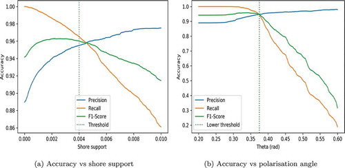
Where $\otimes$ represent signal cross-correlation between the sequences and $\hat{x}$ is the zero mean shifted signal of $x$. Water segments are filtered by comparing the calculated shore support with an estimated threshold. Agricultural fields appear barren during summer. Data near the Ananthapur region, which is mostly dry during summer analysed for estimating threshold for shore support. For the selected area of interest, the generated polygons were validated against global water layer (Pekel et al. 2016). The optimum value is fixed by sweeping the parameter against F1 Score. Figure 7a shows the variation of accuracy parameters (Precision, Recall and F1 score) against shore support for filtering the segments.

Figure 7. parameter sweep for determining thresholds

4.4.2. Polarization angle

The backscattered signal is characterized by its polarization. Microwave radiation undergoes polarization rotation characteristic of the target. Barren lands and other lookalikes are eliminated by considering the polarization rotation incurred during backscattering. The backscattered power received in each polarization (VV & VH) is converted into a polar coordinate system ($r,\varphi$) using equations 18(18) $\theta =ta{n}^{-1}(\frac{p_{vv}}{p_{vh}})$(18) & 19(19) $r=\sqrt{p_{vv}^2+p_{vh}^2}$(19) and its mean over the segmented region is used to estimate the polarization angle.

(18) $\theta =ta{n}^{-1}(\frac{p_{vv}}{p_{vh}})$(18)

(19) $r=\sqrt{p_{vv}^2+p_{vh}^2}$(19)

Figure 6 plots the distribution of $\theta$ and $r$ estimated from water bodies and look alikes. It is observed that backscatter from water bodies are more confined in polarization angle compared to other features. The polarization angle measured for each segment is compared with n lower threshold below which the segment is discarded. Variation of accuracy by sweeping the threshold value is plotted in Figure 7b.

4.4.3. Shadow and low grazing areas

Due to the side looking nature, shadows are inevitable in SAR images. Low grazing and shadows appear as low backscatter areas. Shadow estimation algorithms using DEM for RADAR images is described in (Prasath and Haddad 2013; Zhu et al. 2016). A slightly modified approach using trigonometric computation, optimized for segment-based processing is used. Since the scenario here is to check whether a given segment is a shadow, the whole image need not be processed. The algorithm does a walk around in the DEM corresponding to the detected low backscatter region to detect a possible shadow casting structure. For the detection of a shadow cast by hills and other structures, DEM is used along with the radar heading angle and look angle (Look angle from geoid, incidence angle and head angle from satellite metadata of the product). The extent of the image is computed and maximum height is calculated perpendicular to the heading angle and DEM is checked against the minimum height that can cast a shadow. If DEM is grater than minimum height, then the segment is flagged as a shadow. For a DEM with pixel size $l_x\times l_y$ let $p_0$ be the centroid of the segment, $\delta p_{max}$ be the maximum extent of the segment from $p_0$ and $\varphi$ be the heading angle and $\theta$ be the incidence angle on ellipsoid at $p_0$. A line P is drawn from $p_0$ towards the satellite for a distance of $2\times \delta p_{max}$.

(20) $\hat{p}=(l_{x}sin(\varphi ),l_{y}cos(\varphi ))$(20)

(21) $P=\left\{p_0+n\stackrel{⌢}{p}\left|n\in \left\{0,1,\dots ⌈\frac{\delta p_{max}}{\left|\hat{p}\right|}⌉\right\}\right.\right\}$(21)

(22) $H=\{d(p_0,q)\times sin(\theta )|q\in P\}$(22)

$where$

(23) $d(p,q)=\sqrt[2]{|p-q{|}^2}$(23)

(24) $H_{el}=\{DEM(p)|\mathrm{\forall }p\in P\}$(24)

(25) $P_{sh}=\mathrm{a}\mathrm{n}\mathrm{y}(H_{el}>H)$(25)

$d(p,q)$is the Euclidean distance. Every element in $H$ is compared with height $H_{el}$ from DEM and the region is flagged as a shadow, if any element in $H_{el}$ is greater than the corresponding element in $H$ (equation 25(25) $P_{sh}=\mathrm{a}\mathrm{n}\mathrm{y}(H_{el}>H)$(25) ).

Surfaces having low grazing angle are more likely to give low back scatter. Segments which are formed due to low grazing angle are detected by estimating its average grazing angle over the segmented region. Grazing angle is determined from the local incidence angle generated from DEM using SNAP.

4.5. Segment classifier

Assuming each derived parameters are mutually independent, segments are filtered using each estimated parameters. Each connected segment with its calculated shore support, grazing angle, polarization angle and shadow casting is given to a logical classifier to qualify the segment as a water body. The logical classifier is of the form

NOT(shadow) AND Grazing angle > 20

AND Shore_support > 0.004 AND theta > 0.37

Where the thresholds are estimated using parameter sweep taking into account the accuracy of classification using F-score as described in section 4.4. The entire algorithm was implemented in python using a multi-threaded approach as described in (Bipin et al. 2018).

5. Results

For estimating the accuracy, the generated water bodies were validated against near time optical satellite images and Global water dynamics data. Global water dynamics data derived from 35 years of Landsat satellite images were provided by Ref. global surface water. The data consist of maximum extent, Occurrence, seasonality, recurrence, transitions and change from 1984 to 2018. RS2A LISS-IV MX and S2A MX data collected at a near date with SAR data is used as reference for segmentation accuracy calculations. The search levels are configured to allow all dark regions across the scene by allowing commissions. The detection accuracy is estimated by segmenting different water bodies spread across all incidence angles (across the scene) and seasons. Twelve data sets for every month in the region near Hyderabad were used for the analysis. Forty-two water bodies which were distributed across the scene were selected and observed on all the data sets. AOIs were drawn using shapefile in geographic latitude and longitude coordinates so as to precisely identify the feature in multiple geo-referenced optical and SAR images. Distribution of AOIs for the selected water bodies is shown in Figure 3 All permanent water bodies (seasonality = 12 inferred from Global water occurrence data) were observed and were consistently detected. Distortions were observed in some water bodies during the rainy season which could be attributed to backscattering from rain cells (Alpers et al. 2016).

As water bodies are very dynamic in nature, validation requires reference data which is acquired in near time. For comparing the accuracy of segmentation, the results were compared with near time optical data, the algorithm output was validated against manually vectored water layer from S2A MX and RS2A LISS-IV MX collected near Ananthapur for the month of November. Figures 4 d & 4 cshows the AOIs drawn over identified water bodies using optical data for validation. Results are analysed in terms of F-score and tabulated in Table 3. Results obtained over two selected water bodies is shown in Figure 8. Microwave SAR backscatter is found to be highly sensitive to aquatic vegetation. Presence of traces of aquatic vegetation which is hard to detect in optical images was found to give high backscatter in SAR image.

Figure 8. SBIA output and manually drawn layers over LISS4 MX and Sentinel-1 SAR data

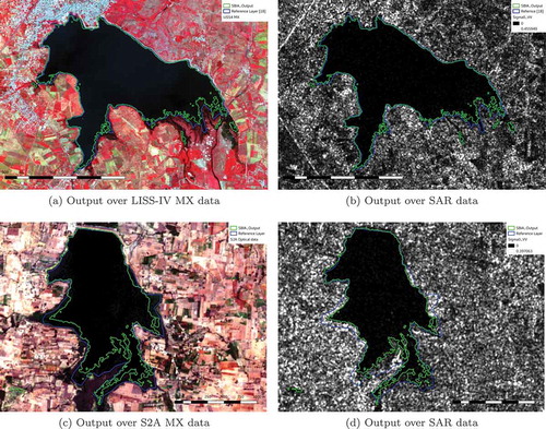
Table 3. Segmentation Accuracy

Optical sensor	Count	Ref area (ha)	Precision	Recall	F-1 score
RS2A LISS-IV MX	18	476.5	0.967	0.897	0.930
S2A MX	15	426.6	0.982	0.881	0.929

The performance of SBIA is compared with widely used threshold based and region growing methods. Watershed (Soille and Ansoult 1990; Vincent and Soille 1991) and Random walker (Grady 2006) are two region growing methods for image segmentation. The algorithms which is part of Scipy (Virtanen et al. 2020) library available with python language was used to estimate its performance in segmenting SAR data. Figure 9 gives the comparison of segmenting SAR images using watershed, Random walker, and the proposed level-based search. Manually vectorized layers from S2A MX and RS2A LISS-IV MX collected near Ananthapur for the month of November are used as reference. It can be observed that the region growing algorithms grow beyond the boundaries in many cases. This could be attributed to the presence of speckle noise which makes it difficult to estimate proper boundaries with a single homogeneous model for the waterbody. For the selected AOIs, water bodies are extracted using Otsu’s threshold, random walker and watershed. The accuracy in terms of precision, recall and f1 score for each algorithm is tabulated on Table 4. Comparing the accuracy with Table 3, it is evident that SBIA have better segmentation accuracy.

Figure 9. Segmentation of SAR image using watershed, Random Walker and SBIA in SAR data overlaid on SAR and corresponding optical image

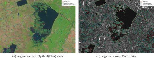
Table 4. Accuracy of other algorithms evaluated near Ananthapur region

Algorithm	Precision	Recall	F1 score
Otsu	0.496	0.986	0.660
Random walker	0.855	0.927	0.890
Watershed	0.871	0.922	0.896

To estimate the overall accuracy, the region near Bangalore and Hyderabad where numerous water bodies were present was chosen for the month of November. November is chosen as it is the time after the monsoon season (June to September) which accounts for more than 80% of annual rainfall in the region. During monsoon season, a lot of unaccounted surface water bodies could be present, which may pose difficulty in validation with the reference derived from optical data. The results obtained were validated against global water extend data. The results are summarized in terms of the area analysed, precision, recall and F1 score in Table 5. Details about extent, total water bodies, total water body area for each reference area and the validation results are summarized in Table 1. Figure 4 gives the AOI drawn over Bengaluru region for validation and the result obtained.

Table 5. Accuracy of estimation

Area name	Total area (ha)	True positive (ha)	Precision	Reacll	F1
Bangalore	1.29e+06	2.442e+04	0.9889	0.893	0.9385
Hyderabad	6.979e+04	1.024e+04	0.9998	0.938	0.9679

6. Conclusion

SBIA is found to be giving promising results in water body extraction from SAR images. The results were compared and found in good agreement with water bodies extracted from optical data of comparable resolution. The algorithm is capable of detecting many temporary and seasonal water bodies enabling studying of short-term dynamics in water bodies. Aquatic vegetation is found to create large errors in the estimated area at particular times of the year.

Though the algorithm is based on fixed levels estimated from histogram and number of segments estimated from search in selected AOI, SBIA has reliably detected water bodies across the scene over seasons. This could be attributed to the reliable nature of SAR backscatter observation and uniqueness of water bodies at microwave frequencies. Application search using three-level model based on fixed thresholds in single polarization is limited to extraction of water bodies alone. The methodology is found to overcome speckle and low feature dimension which pose major challenges in SAR image processing. The three-level model-based search can be extended to other features and datasets (polarimetric and multi-temporal) using widely used classification algorithms instead of fixed threshold-based levels.

Acknowledgements

The authors would like to thank Shri Santanu Chowdhury, former director National Remote Sensing Centre, Hyderabad for his inspiration and guidance in carrying out this work. We thank Water Body Information System Group, NRSC, Hyderabad for the help and support extended in this work. The authors also like to thank Andhra University, Visakhapatnam and all our colleagues who have cooperated with this work.

Disclosure statement

No potential conflict of interest was reported by the authors.

References

- Abello, J., P. M. Pardalos, and M. G. C. Resende. 2013. “Handbook of Massive Data Sets.” Massive Computing. Springer US. https://books.google.co.in/books?id=NfcGCAAAQBAJ
- Alpers, W., B. Zhang, A. Mouche, K. Zeng, and P. W. Chan. 2016. “Rain Footprints on C-band Synthetic Aperture Radar Images of the Ocean - Revisited.” Remote Sensing of Environment 187: 169–185. doi:10.1016/j.rse.2016.10.015.
- Anand, N. S., R. Marappan, and G. Sethumadhavan. 2018. “Performance Analysis of SAR Image Speckle Filters and Its Recent Challenges.” In 2018 IEEE International Conference on Computational Intelligence and Computing Research (ICCIC), Madurai, India, December, 1–4. doi: 10.1109/ICCIC.2018.8782425
- Bechtel, B., A. Ringeler, and J. Bohner. 2008. “Segmentation for Object Extraction of Trees Using MATLAB and SAGA.” SAGA–Seconds Out, Hamburger Beitrage Zur Physischen Geographie Und Landschaftsokologie. Univ. Hamburg, Inst. fur Geographie 1–12.
- Bipin, C., C. V. Rao, P. V. Sridevi, S. Jayabharathi, and B. G. Krishna. 2018. “A Multi Threaded Feature Extraction Tool for SAR Images Using Open Source Software Libraries.” ISPRS - International Archives of the Photogrammetry, Remote Sensing and Spatial Information Sciences XLII-5, Dehradun, India, 155–160. https://www.int-arch-photogramm-remote-sens-spatial-inf-sci.net/XLII-5/155/2018/
- Blaschke, T. 2010. “Object Based Image Analysis for Remote Sensing.” ISPRS Journal of Photogrammetry and Remote Sensing 65 (1): 2–16. doi:10.1016/j.isprsjprs.2009.06.004.
- Cantrell, C. D. 2000. Modern Mathematical Methods for Physicists and Engineers. New York, NY, USA: Cambridge University Press.
- ESA. 2018. “Copernicus Sentinel Data [2017-2018] Processed by ESA.” https://sentinels.copernicus.eu/web/sentinel/missions/sentinel–1
- Geldsetzer, T., and J. J. Yackel. 2009. “Sea Ice Type and Open Water Discrimination Using Dual Co-polarized C-band SAR.” Canadian Journal of Remote Sensing 35 (1): 73–84. doi:10.5589/m08-075.
- Goodman, J. W. 1975. Statistical Properties of Laser Speckle Patterns. 9–75. Berlin, Heidelberg:Springer Berlin Heidelberg. doi:10.1007/978-3-662-43205-1_2.
- Grady, L. 2006. “Random Walks for Image Segmentation.” IEEE Transactions on Pattern Analysis and Machine Intelligence 28 (11): 1768–1783. doi:10.1109/TPAMI.2006.233.
- Hua-Xin, Z. H. A. N. G., L. I. U. Na, L. I. U. Ren-Xi, Z. H. A. N. G. Feng, and Y. I. N. Tian-He. 2011. “Cas- Caded Union Algorithm for Polygon Set Based on Grid.” Computer Engineering 37 (6): 38. http://www.ecice06.com/EN/abstract/article_20521.shtml
- Lee, D. T., and B. J. Schachter. 1980. “Two Algorithms for Constructing a Delaunay Triangulation.” International Journal of Computer & Information Sciences 9 (3): 219–242. doi:10.1007/BF00977785.
- Lee, J. S., J. H. Wen, T. L. Ainsworth, K. S. Chen, and A. J. Chen. 2009. “Improved Sigma Filter for Speckle Filtering of SAR Imagery.” IEEE Transactions on Geoscience and Remote Sensing 47 (1): 202–213. doi:10.1109/TGRS.2008.2002881.
- Lee, J.-S. 1983. “Digital Image Smoothing and the Sigma Filter.” Computer Vision, Graphics, and Image Processing 24 (2): 255–269. doi:10.1016/0734-189X(83)90047-6.
- Loew, A., and W. Mauser. 2007. “Generation of Geometrically and Radiometrically Terrain Corrected SAR Image Products.” Remote Sensing of Environment 106 (3): 337–349. doi:10.1016/j.rse.2006.09.002.
- NASA. n.d. “The Shuttle Radar Topography Mission (SRTM) 1 Arc-Second Global DEM.” https://www2.jpl.nasa.gov/srtm/
- Pekel, J.-F., A. Andrew Cottam, N. Gorelick, and A. S. Belward. 2016. “High-resolution Mapping of Global Surface Water and Its Long-term Changes.” Nature 540 (7633): 418–422. doi:10.1038/nature20584.
- Pham-Duc, B., C. Prigent, and F. Aires. 2017. “Surface Water Monitoring within Cambodia and the Vietnamese Mekong Delta over a Year, with Sentinel-1 SAR Observations.” Water (Switzerland) 9 (6): 1–21.
- Prasath, V. B. S., and O. Haddad. 2013. “Radar Shadow Detection in SAR Images Using DEM and Projections.” CoRR 1830. http://arxiv.org/abs/1309
- Silveira, M., and S. Heleno. 2008. “Water/land Segmentation in SAR Images Using Level Sets.” In 2008 15th IEEE International Conference on Image Processing, October, San Diego, CA, USA, 1896–1899. doi: 10.1109/ICIP.2008.4712150
- Silveira, M., and S. Heleno. 2009. “Separation between Water and Land in SAR Images Using Region-Based Level Sets.” IEEE Geoscience and Remote Sensing Letters 6 (3): 471–475. doi:10.1109/LGRS.2009.2017283.
- Small, D., and A. Schubert. 2008. “Guide to ASAR Geocoding.” Rsl-Asar-Gc-Ad 1: 36.
- Soille, P. J., and M. M. Ansoult. 1990. “Automated Basin Delineation from Digital Elevation Models Using Mathematical Morphology.” Signal Processing 20 (2): 171–182. doi:10.1016/0165-1684(90)90127-K.
- Sun, S., R. Liu, C. Yang, H. Zhou, J. Zhao, and J. Ma. 2016. “Comparative Study on the Speckle Filters for the Very High-resolution Polarimetric synthetic Aperture Radar Imagery.” Journal of Applied Remote Sensing 10 (4): 1–13. doi:10.1117/1.JRS.10.045014.
- Vincent, L., and P. Soille. 1991. “Watersheds in Digital Spaces: An Efficient Algorithm Based on Immersion Simulations.” IEEE Transactions on Pattern Analysis and Machine Intelligence 13 (6): 583–598. doi:10.1109/34.87344.
- Virtanen, P., R. Gommers, T. E. Oliphant, M. Haberland, T. Reddy, D. Cournapeau, E. Burovski, et al. 2020. “Scipy 1.0: Fundamental Algorithms for Scientific Computing in Python.” Nature Methods 17 (3): 261–272.
- Wang, X., and L. Li. 2015. “Speckle Suppression of Synthetic Aperture Radar Image with Empirical Mode Decomposition and Principal Component Analysis Based on Noise Energy Estimation.” Journal of Applied Remote Sensing 9 (1): 1–12. doi:10.1117/1.JRS.9.095073.
- Zhang, G., and W. Zhensen. 2010. “Effect of Apertures on the Speckle Size from Rough Surfaces.” In Proceedings of the 9th International Symposium on Antennas, Propagation and EM Theory, Guangzhou, China, November, 730–733. doi: 10.1109/ISAPE.2010.5696571
- Zhu, H., J. Yin, D. Yuan, X. Liu, and G. Zhang. 2016. “Dem-based Shadow Detection and Removal for Lunar Craters.” In 2016 IEEE International Geoscience and Remote Sensing Symposium (IGARSS), Beijing, China, July, 6906–6909. doi: 10.1109/IGARSS.2016.7730802