Modelling spatial processes in quantitative human geography

ABSTRACT

We discuss the nature of processes relating to human behaviour and how to model such processes when they vary over space. In so doing, we describe the role of local modelling and how the bandwidth parameter, a component of multiscale geographically weighted regression, can inform on the spatial scale over which processes are relatively constant. To do this, we translate properties of spatial data, such as heterogeneity and spatial dependency into the realm of spatial processes. We argue that the modelling of spatially varying processes has important ramifications for how we see the world.

KEYWORDS:

• Spatial processes
• local statistical models
• multiscale geographically weighted regression
• spatial scale
• reproducibility

1. Introduction

The study of processes in quantitative human geography has a long history, nicely encapsulated by Hay and Johnston (1983). However, as ‘process’ is often interpreted as a sequence of events leading to a particular outcome, studies in quantitative human geography that focus on processes are often hampered by a lack of temporal data. Typically, data are observed at multiple locations but in only one time period. In contradistinction, studies in physical geography and economics often have the luxury of data sets that have a rich temporal dimension, although sometimes with limited spatial resolution. Under the assumption that processes are spatially stationary (the usual scenario in the physical sciences), the lack of spatial resolution is not a hindrance to the identification of processes if sufficient time-series data are available at even just a single location. However, what if the processes being studied are NOT spatially stationary (a likely scenario in the social sciences)? In this situation, can we then replace the variations we typically measure in the temporal dimension with variations we observe in the spatial dimension to infer something about such processes? In the remainder of this paper, we explore this situation.

Throughout most of its long history, human geography has been primarily concerned with data. Initially, the focus was on mapping data, but during the 1960s, statistical methods were introduced and the analysis of spatial data came to the fore, exemplified by measures of spatial dependence and point pattern analysis. The idea that we could quantify issues such as the degree to which similar data values clustered was appealing and spurned a huge literature (Moran 1948, 1950; Whittle 1954; Matheron 1963; Paelinck and Klaassen 1979; Cliff and Ord 1981; Hubert, Golledge, and Costanzo 1981; Anselin 1988, 1995; Getis 1991; Getis and Ord 1992; Ord and Getis 1995, 2001; Griffith 2003). Around this time, human geography developed its first, and possibly only, ‘law’ which again focused on data – ‘everything is related to everything else, but near things are more related than distant things’ Tobler 1970. Although this is not really a ‘law’ but an empirical observation, it stands as a description of a regularity that has achieved the status of a ‘law within human geography and encapsulates the concept of data spatial dependency succinctly.

As human geography’s ‘quantitative revolution’ proceeded and spatial analysis became both commonplace and more mature, the traditional emphasis of the discipline on data gradually gave way to a competing interest in processes. It became insufficient to describe how some variable was distributed over space and the emphasis shifted towards providing an explanation of why a variable was distributed in a certain way over space. This why question led to an interest in the process or processes causing the observed distribution of data. As Harvey (1967) noted: ‘ … different processes become significant to our understanding of spatial patterns at different scales’. (p. 71–72), an observation expounded upon decades later by Manley, Flowerdew, and Steel (2006):

Spatial distributions are based on processes taking place in geographical space. A mapped pattern may reflect several distinct processes, each of which may affect a different area and operate at a different scale. The challenge for the spatial analyst is to identify these processes and evaluate their importance from the spatial pattern observed. (p. 143)

As a consequence of the growing interest in process rather than form, came a focus on the development of models, particularly explicitly spatial models, such as spatial regression models (Anselin, 1988, 2002, 2009; Griffith & Csillag, 1993; Haining, 1993; Tiefelsdorf, 2000; Gelfand et al., 2003; Haining, 2003; Waller & Gotway, 2004; LeSage & Pace, 2010; Banerjee et al., 2014) and spatial interaction models (Olsson, 1970; Wilson, 1971; Fotheringham, 1983a; 1983b; 1984; Fotheringham & O’Kelly, 1989). Although spatial models have several purposes, undoubtedly the main one is to try to uncover what factors affect the spatial distribution of a particular variable; or, rather crudely, to answer the question: ‘Why are some values high and why are some low?’. This is typically done by making inferences about how covariates influence the dependent variable through the estimates of the parameters obtained in the calibration of the model.

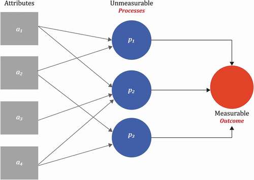
The focus of this paper is encapsulated in Figure 1. In whatever subject matter we study, we understand that there are processes, which here we think of as being interactions between attributes, that lead to a certain outcome that we measure. In the physical sciences such processes can often be deduced from first principles, but in the social sciences such processes are often unknown and have to be inferred from the measured outcomes. This latter is not ideal because of the problem of equifinality – the same outcome can result from different processes – but it underlies the complexity of dealing with the actions of human beings where universal laws of behaviour are rare. However, it can be argued that making inferences about properties of processes is better than ignoring them.¹ Here, we focus on a situation with even greater complexity – where the processes being examined may not be spatially stationary, again a situation which highlights the difference between modelling the physical environment from the human environment.

Figure 1. Attributes, processes and outcomes.

2. Modelling spatial processes

From the origins of the quantitative ‘turn’ across many social sciences came a focus on relationships between attributes with regression-based models exemplified by equation (1)(1) $y={\beta }_0+{\beta }_1{x}_1+{\beta }_2{x}_2+\dots +{\beta }_n{x}_n+\in$(1) :

(1) $y={\beta }_0+{\beta }_1{x}_1+{\beta }_2{x}_2+\dots +{\beta }_n{x}_n+\in$(1)

where $y$ is the variable of interest, $x_1,x_2,\dots ,x_n$ are covariates, ${\beta }_0$ is the intercept, ${\beta }_1,{\beta }_2,\dots ,{\beta }_n$ are slope parameters and ϵ is a random error term. Each of the slope parameters represents the conditional effect of a change in the respective covariate on $y$ and hence is an indicator of a specific process operating to contribute to the value of $y$ observed at each location. Consequently, it is from the estimates of these parameters obtained in the calibration of the model that we make inferences about each of the processes that together create the observed distribution of $y$.

It quickly became apparent that models of the format of equation (1)(1) $y={\beta }_0+{\beta }_1{x}_1+{\beta }_2{x}_2+\dots +{\beta }_n{x}_n+\in$(1) were often inadequate when applied to spatial data because the distribution of epsilon generally exhibited significant positive spatial autocorrelation, violating the requirement of Gaussian regression that the error terms be identically and independently distributed. If the error terms exhibited significant clustering, how could they be independently distributed? This prompted the development of various forms of what became known as spatial regression models exemplified by that of a spatial error model shown in equation (2)(2) $y={\beta }_0+{\beta }_1{x}_1+{\beta }_2{x}_2+\dots +{\beta }_n{x}_n+\hspace{0.17em}\lambda \left(W\right)+\mu$(2) (Anselin, 1988; Gibbons & Overman, 2012; Kelejian & Prucha, 1998, 1999; Lesage, 2016; LeSage & Pace, 2010).

(2) $y={\beta }_0+{\beta }_1{x}_1+{\beta }_2{x}_2+\dots +{\beta }_n{x}_n+\hspace{0.17em}\lambda \left(W\right)+\mu$(2)

where ϵ is a vector of spatially autocorrelated error terms, $\lambda$ is a parameter estimated to measure the spatial autocorrelation in the error term ϵ, $W$is a spatial weights matrix, $\mu$ is a vector of independent and identically distributed (i.i.d.) errors, $x_1,x_2,\dots ,x_n$are covariates and ${\beta }_0,{\beta }_1,\dots ,{\beta }_n$are parameters to be estimated given data on $y$ and $x_1,\dots ,x_n$.

A fundamental assumption to OLS or spatial regression models (and to almost any other form of model used in Geography prior to 2000) is that the processes being inferred through the parameters of the model are stationary over space. That is, we typically collect data from various spatial locations and use all these data to calibrate a model of the form of either equation (1)(1) $y={\beta }_0+{\beta }_1{x}_1+{\beta }_2{x}_2+\dots +{\beta }_n{x}_n+\in$(1) or (2(2) $y={\beta }_0+{\beta }_1{x}_1+{\beta }_2{x}_2+\dots +{\beta }_n{x}_n+\hspace{0.17em}\lambda \left(W\right)+\mu$(2) ) to produce a single estimate of each parameter. The implicit assumption is therefore that the process represented by a single parameter in the model must be stationary over space. We now question this assumption and examine the ramifications of relaxing it.

Until recently, there existed a logical inconsistency in spatial data analysis whereby, while it was taken as given that spatial data exhibited heterogeneity, spatial processes were assumed to be homogeneous. This belief was presumably a hold-over from borrowing quantitative techniques which had their origins in the natural sciences and where processes are typically stationary over space. Whereas most physical processes are invariant to location, social science processes, involving the beliefs, preferences and actions of human beings, are likely to vary according to location. Indeed, a huge literature exists supporting this idea (Chetty and Hendren 2018; Sampson 2019; Darmofal 2008; Plaut, Markus, and Lachman 2002; Escobar 2001; Diez-Roux 1998, 2001). Consequently, various local modelling paradigms have been developed by geographers and statisticians which challenge the assumption of spatial process stationarity by allowing the parameters in a model to vary over space, as typified by equation (3)(3) $y_i={\beta }_{0i}+{\beta }_{1i}{x}_{1i}+{\beta }_{2i}{x}_{2i}+\dots +{\beta }_{ni}{x}_{ni}+{\in }_i$(3) .

(3) $y_i={\beta }_{0i}+{\beta }_{1i}{x}_{1i}+{\beta }_{2i}{x}_{2i}+\dots +{\beta }_{ni}{x}_{ni}+{\in }_i$(3)

where $x_{ni}$ is an observation of the $n^{th}$ explanatory variable at location i, ${\beta }_{ni}$ is the n^th parameter estimate which is now specific to location i, and ϵ_i is a random error term. In this representation of the world, spatial process variation is accommodated by the flexibility of allowing each parameter to vary over space. Several frameworks have been established that allow the modelling of spatially varying processes, such as Geographically Weighted Regression (GWR); Bayesian Spatially Varying Coefficients Models (SVCM), Eigenvector Spatial Filtering (ESF) and Spatially Clustered Coefficient models (SCC) (Banerjee et al., 2014; Fotheringham et al., 2003; Fotheringham et al., 2017; Gelfand et al., 2003; Griffith, 2008; Li & Sang, 2019; Murakami et al., 2017). . Although these modelling frameworks differ in how they represent spatially varying processes, they share the basic idea that processes might vary over space and that global model representations such as those in equations (2)(2) $y={\beta }_0+{\beta }_1{x}_1+{\beta }_2{x}_2+\dots +{\beta }_n{x}_n+\hspace{0.17em}\lambda \left(W\right)+\mu$(2) and (3(3) $y_i={\beta }_{0i}+{\beta }_{1i}{x}_{1i}+{\beta }_{2i}{x}_{2i}+\dots +{\beta }_{ni}{x}_{ni}+{\in }_i$(3) ) are inadequate in such circumstances. Also common to all four frameworks is the assumption of process spatial dependency. That is, if processes do vary over space, they are unlikely to vary randomly but are likely to follow a process-based equivalent to Tobler’s Law regarding the prevalence of spatial data dependence. We now examine why processes might vary over space and the ramifications of such process spatial nonstationarity.

3. The role of spatial context

Given the current interest in the development of local statistical methods that allow the modelling of spatially nonstationary processes, it is pertinent to ask why processes might vary over space. After all, they typically do not in the physical sciences so why might they in the social sciences? The answer to this is not an easy one as the processes themselves are hidden, and we can only make inferences about them. Consequently, although there is a substantial amount of empirical evidence that supports the notion that many processes do vary over space, it is difficult to be absolutely certain that our models are not picking up some spurious cause of parameter variation. Equally, we have little theory to guide us on this issue and we have to rely largely on supposition and hypotheses. That said, there is a vast amount of literature which suggests that ‘place matters’ and that local ‘context’ can have a major impact on people’s beliefs, preferences, and actions (Agnew, 2014; Duncan & Savage, 2006; Golledge, 1997; Goodchild, 2011; Gould, 1991; Hartshorne, 1939a, 1939b; Harvey & Wardenga, 2006; Pred, 1984; Relph, 1976; Sayer, 1985; Thomae, 1999; Tuan, 1979; Winter et al., 2009; Winter & Freksa, 2012). Such a link between place and behaviour can arise if people are influenced by the people they talk to on a regular basis or by their local media or if they face long-term conditions that are particular to certain locales and which shape people’s outlooks on issues. Evidence for this on a large scale can be seen in geographic variations in preferences for certain types of foods, music, house styles, political parties, etc. (Walker and Li 2007; Enos 2017; Escobar 2001; Shortridge 2003; Agnew, 1996; Braha and De Aguiar 2017; and Fotheringham et al. 2021). However, despite a wealth of evidence that place matters and that location can help shape preferences and actions, an alternative viewpoint is that spatial context does not exist and that what is referred to as ‘context’ is merely a catch-all term for those covariates not included in the model either because they have not been conceived of having importance or because they are difficult to measure McAllister 1987.

It is difficult to argue definitively for either viewpoint because even though many sociological and psychological studies have pointed to the relevance of context (Enos 2017; Plaut, Markus, and Lachman 2002; Rentfrow, Jokela, and Lamb 2015; Krug and Kulhavy 1973) and a great number of geographical studies have espoused the role of location in affecting behaviour from a theoretical viewpoint (Blake, 2001; Books & Prysby, 2016; Carsey, 1995; Chandola et al., 2005; Rousseau & Fried, 2001; Snedker et al., 2009), it could equally be claimed that whatever the effects of location are, they could, theoretically, be measured and incorporated into the model. Whether context is a ‘real’ effect or simply a catch-all for variables that cannot be or have not been measured therefore remains elusive, but whatever its source, the ability to capture ‘context’ within local models is better than not accounting for it as is the case in traditional global models. In global models, the omission of an important explanatory variable will create misspecification bias in the parameter estimates associated with any covariate that has some degree of covariance with the omitted variable. As an example of this, and the calculation of the explicit degree of misspecification bias caused by an omitted variable (see Fotheringham 1983a, 1984). Alternatively, If the processes being modelled do vary over space, but they are modelled with a traditional global model, the latter will be grossly misspecified and the estimates of the parameters derived from this model will simply represent an average process and will be as unrepresentative of the spatial varying processes as is, for example, the mean annual rainfall of the United States as a measure of the annual rainfall in each county. On balance, the strategic view would appear to be to assemble as comprehensive a set of covariates as possible and to calibrate a local model using these covariates. This will reduce any misinterpretation of the local intercept as a measure of context and the model will default to a global one in the situation where the processes are stationary over space.

4. The spatial scale of process nonstationarity

Local models of the type shown in equation (3)(3) $y_i={\beta }_{0i}+{\beta }_{1i}{x}_{1i}+{\beta }_{2i}{x}_{2i}+\dots +{\beta }_{ni}{x}_{ni}+{\in }_i$(3) are able to capture spatially varying processes through the estimation of location-specific parameter estimates. However, two of the local modelling frameworks mentioned above, GWR and SVCM, also provide a bandwidth parameter which denotes the spatial scale over which a process varies. In the case of the multiscale versions of GWR and SVCM, covariate-specific bandwidth parameters are estimated, and in the case of MGWR, confidence intervals for these bandwidths can be calculated. We now discuss what the notion of a ‘bandwidth’ in (M)GWR means in terms of the spatial scale over which a process varies.

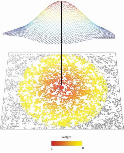
In the (M)GWR framework, a local model is calibrated for each location so that location-specific parameters and various diagnostics are produced. Typically, there exists only one measurement of each variable at each location so data are ‘borrowed’ from nearby locations and weighted according to the distance each location is from the regression point with weights falling as distance increases (Fotheringham, Brunsdon, and Charlton 2003). The weighting is controlled by a distance-decay parameter, or bandwidth, so that the weights range between 1 (at the regression point) 0 (at the bandwidth). This process is summarized in Figure 2.

Figure 2. Spatial weighting in geographically weighted regression.

The optimal bandwidth is a trade-off between the amount of bias in the local parameter estimates and their uncertainty (or variance). Bias in the local parameter estimates is caused by borrowing data from other locations where the processes that produced those data may not be the same as those that are being estimated at the regression location. Assuming that if processes vary over space, this variation is unlikely to be random and will exhibit some degree of spatial dependency so that bias in local parameter estimates will tend to increase when data are borrowed from more distant locations. Uncertainty in the local parameter estimates exists because we are using a sample of data from which to calculate these estimates and this uncertainty will decrease as more data are borrowed in each local regression. Hence, small bandwidths generate lower parameter bias but increased uncertainty whereas large bandwidths generate greater parameter bias but lower uncertainty. This situation is captured in Figure 3. Note that the range of data-borrowing for the local regression at i, the bandwidth, can be estimated in terms of a physical distance or in terms of the number of nearest neighbours. It is generally more intuitive, and eases comparisons across studies, if the latter is used.

Figure 3. Optimal bandwidth selection in GWR.

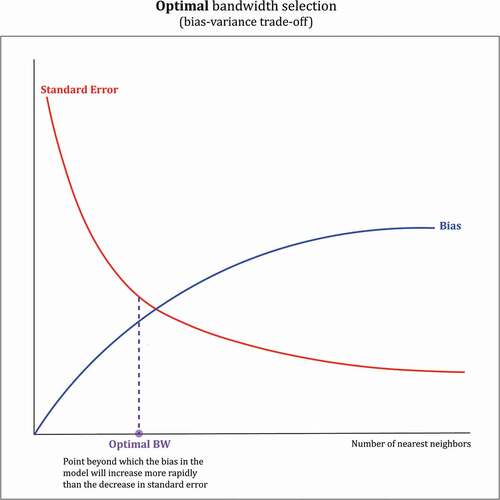
As Yu et al. (2020) show, the bandwidth at which the bias-uncertainty trade-off in local parameter estimates is optimized can be found by minimizing a corrected Akaike Information Criterion statistic which is the preferred option in MGWR and GWR software routines (see, for example, MGWR 2.2 software that can be downloaded from https://sgsup.asu.edu/sparc/mgwr and runs on both Windows and MacOS platforms). Essentially, as locations from which data are borrowed are added to the local regressions, the reduction in parameter uncertainty outweighs the increase in parameter bias until a point is reached (the optimal bandwidth) at which the increase in parameter bias outweighs the reduction in bias. If the process being modelled has a high degree of spatial variability, the bandwidth will be small; if the process has low spatial variability, the bandwidth will be large. A global process will result in an infinitely large bandwidth and a global model is therefore a special case of a local model in which all the processes being modelled have infinitely large bandwidths which gives a weight of 1 to all data points. Consequently, the optimized bandwidth for each covariate that is reported in an MGWR calibration provides useful information on the spatial scales over which different processes vary (see Fotheringham et al. 2020 for an example of this in a voting context). In this sense, the spatial scale referred to by a covariate-specific optimal bandwidth represents the spatial extent over which a process is relatively stable. Given processes may vary over space, we need some comparative measure of their relative variability and for this we chose the point at which the amount of bias in the local parameter estimates exceeds the amount of uncertainty in the local estimates as measured by their standard error (for more details refer to Yu et al. 2020). Hence, the optimal bandwidth for each covariate denotes the range around a location i where data borrowed for the local regression at i reduce parameter uncertainty more than they increase parameter bias. Beyond the bandwidth, the addition of further data to the regression at i would increase bias more than they would decrease uncertainty. This is a measure of a property of spatially varying processes which can be compared across covariates to inform on the spatially varying nature of each local process.

5. Summary and implications

The premise of this paper is that there are reasons to suspect that the processes producing the data we observe about human beings and their actions may not be stationary due to the influence of spatial context. This is a relatively new perspective in quantitative spatial sciences. Should social processes exhibit spatial nonstationarity, what are the ramifications of this? Should we ignore this possibility and continue calibrating global models which assume spatial stationarity and which will yield only average statements of spatially varying processes? This paper takes the view that we should try to model and explore any spatial process of nonstationarity as an interesting and potentially useful facet of human behaviour. It further takes the view that if processes do vary over space because of spatial contextual effects, they are unlikely to vary randomly and almost certainly will exhibit some degree of spatial dependency – processes at locations in close proximity are more likely to be similar than are processes at locations farther apart. We can model the degree to which different processes vary over space through multiscale geographically weighted regression, as described above. This local modelling technique produces covariate-specific bandwidths, each of which yields a comparative measure of the spatial extent to which a process is relatively stable. Larger bandwidths indicate processes which are more stable over space and a global model is an extreme case of a local model with extremely large bandwidths.

The development of local models of human behaviour thus provides a powerful set of tools for spatial analysts. However, it does not imply that all processes are spatially varying. Physical processes, for example, those that govern the way matter is formed and behaves, do not vary over space – E does not equal mc^1.5 in some locations! Processes which would seem most likely to exhibit spatial nonstationarity are those which involve human preferences and actions which are susceptible to local contextual effects. Modelling such processes with traditional global models seems unnecessarily restrictive. Why not allow the data to hint at which processes might be spatially varying by calibrating models locally? If the processes being modelled are all global, then nothing is lost as the local model will replicate a global model by making all the optimized bandwidths very large. If the processes do vary across space, however, local models will generate much better predictions of y and generate useful information on the nature of the spatially varying processes by mapping the local parameter estimates and by examining the optimized bandwidth values. Further, if some processes do exhibit spatial nonstationarity, this has profound implications for the current interest in the reproducibility and replicability of geographic research (Goodchild et al., 2020; Kedron et al., 2019, 2020; Sui & Kedron, 2020). If processes are spatially varying, then we cannot expect a model calibrated in one location to be replicated exactly in another location – the processes being modelled might be different in the two locations.

Finally, returning to earlier comments on the focus of geographic studies, the increasing focus on local models of human activity leads us to explore a whole new geography – that of processes. We now have the means to produce maps – not of data – but of processes via the local parameter estimates produced in local models. Spatial processes can be mapped and analysed in much of the same way that spatial data are. Spatial heterogeneity and spatial dependence are two properties of spatial data that are commonly and routinely described in the literature, but these concepts can now be applied to spatial processes.

Disclosure statement

No potential conflict of interest was reported by the author(s).

Additional information

Funding

National Science Foundation under Award 1758786 from the Methodology, Measurement & Stats, Geography and Spatial Sciences Program to A. S. FotheringhamNational Science Board [Award 1758786];

Notes

1. It should be noted that the physical sciences are not immune from the issue of equifinality as the recent debates on climate change demonstrate.

References

- A. Stewart Fotheringham, Ziqi Li & Levi John Wolf (2021). Scale, Context, and Heterogeneity: A Spatial Analytical Perspective on the 2016 U.S. Presidential Election, Annals of the American Association of Geographers, doi:https://doi.org/10.1080/24694452.2020.1835459
- Agnew, J. 1996. “Mapping Politics: How Context Counts in Electoral Geography.” Political Geography 15 (2): 129–146. doi:https://doi.org/10.1016/0962-6298(95)00076-3.
- Agnew, J. A. 2014. Place and Politics: The Geographical Mediation of State and Society. Abingdon: Routledge. doi:https://doi.org/10.4324/9781315756585.
- Anselin, L. 1988. Spatial Econometrics: Methods and Models. Dordrecht: Kluwer Academic Publishers.
- Anselin, L. 1995. “Local Indicators of Spatial Association—LISA.” Geographical Analysis 27 (2): 93–115. doi:https://doi.org/10.1111/j.1538-4632.1995.tb00338.x.
- Anselin, L. 2002. “Under the Hood Issues in the Specification and Interpretation of Spatial Regression Models.” Agricultural Economics 27 (3): 247–267. doi:https://doi.org/10.1111/j.1574-0862.2002.tb00120.x.
- Anselin, L. 2009. “Spatial Regression.” In The SAGE Handbook of Spatial Analysis, edited by A. Fotheringham and P. Rogerson, 254–275. Los Angeles: SAGE Publications, . doi:https://doi.org/10.4135/9780857020130.n14.
- Banerjee, S., B. P. Carlin, and A. E. Gelfand. 2014. Hierarchical Modeling and Analysis for Spatial Data. Boca Raton, Fl: CRC Press.
- Blake, D. E. 2001. “Contextual Effects on Environmental Attitudes and Behavior.” Environment and Behavior 33 (5): 708–725. doi:https://doi.org/10.1177/00139160121973205.
- Books, J., and C. Prysby. 2016. “Studying Contextual Effects on Political Behavior: A Research Inventory and Agenda.” American Politics Quarterly. doi:https://doi.org/10.1177/004478088016002005.
- Braha, D., and M. A. M. De Aguiar. 2017. “Voting Contagion: Modeling and Analysis of a Century of U.S. Presidential Elections.” Plos One 12 (5): e0177970. doi:https://doi.org/10.1371/journal.pone.0177970.
- Carsey, T. M. 1995. “The Contextual Effects of Race on White Voter Behavior: The 1989 New York City Mayoral Election.” The Journal of Politics 57 (1): 221–228. doi:https://doi.org/10.2307/2960280.
- Chandola, T., P. Clarke, R. D. Wiggins, and M. Bartley. 2005. “Who You Live with and Where You Live: Setting the Context for Health Using Multiple Membership Multilevel Models.” Journal of Epidemiology and Community Health 59 (2): 170–175. doi:https://doi.org/10.1136/jech.2003.019539.
- Chetty, R., and N. Hendren. 2018. “The Impacts of Neighborhoods on Intergenerational Mobility I: Childhood Exposure Effects.” The Quarterly Journal of Economics 133 (3): 1107–1162. doi:https://doi.org/10.1093/qje/qjy007.
- Cliff, A. D., and J. K. Ord. 1981. Spatial Processes Models and Applications. London: Pion .
- Darmofal, D. 2008. “The Political Geography of the New Deal Realignment.” American Politics Research 36 (6): 934–961. doi:https://doi.org/10.1177/1532673X08316591.
- Diez-Roux, A. V. 1998. “Bringing Context Back into Epidemiology: Variables and Fallacies in Multilevel Analysis.” American Journal of Public Health 88 (2): 216–222. doi:https://doi.org/10.2105/AJPH.88.2.216.
- Diez-Roux, A. V. 2001. “Investigating Neighborhood and Area Effects on Health.” American Journal of Public Health 91 (11): 1783–1789. doi:https://doi.org/10.2105/AJPH.91.11.1783.
- Duncan, S., and M. Savage. 2006. “Space, Scale and Locality.” Antipode 21 (3): 179–206. doi:https://doi.org/10.1111/j.1467-8330.1989.tb00188.x.
- Enos, R. D. 2017. The Space between Us: Social Geography and Politics. New York, NY: Cambridge University Press.
- Escobar, A. 2001. “Culture Sits in Places: Reflections on Globalism and Subaltern Strategies of Localization.” Political Geography 20 (2): 139–174. doi:https://doi.org/10.1016/S0962-6298(00)00064-0.
- Fotheringham, A. 1983a. “Some Theoretical Aspects of Destination Choice and Their Relevance to Production-Constrained Gravity Models.” Environment and Planning A: Economy and Space 15 (8): 1121–1132. doi:https://doi.org/10.1068/a151121.
- Fotheringham, A., and M. E. O’Kelly. 1989. Spatial Interaction Models: Formulations and Applications. Dordrecht: Kluwer Academic Publishers.
- Fotheringham, A. S. 1983b. “A New Set of Spatial-Interaction Models: The Theory of Competing Destinations.” Environment and Planning A: Economy and Space 15 (1): 15–36. doi:https://doi.org/10.1177/0308518X8301500103.
- Fotheringham, A. S. 1984. “Spatial Flows and Spatial Patterns.” Environment & Planning A 16 (4): 529–543. doi:https://doi.org/10.1068/a160529.
- Fotheringham, A. S., C. Brunsdon, and M. Charlton. 2003. Geographically Weighted Regression: The Analysis of Spatially Varying Relationships.
- Fotheringham, S., W. Yang, and W. Kang. 2017. “Multiscale Geographically Weighted Regression (MGWR).” Annals of the American Association of Geographers 1–19. doi:https://doi.org/10.1080/24694452.2017.1352480.
- Gelfand, A. E., H.-J. Kim, C. F. Sirmans, and S. Banerjee. 2003. “Spatial Modeling With Spatially Varying Coefficient Processes.” Journal of the American Statistical Association 98 (462): 387–396. doi:https://doi.org/10.1198/016214503000170.
- Getis, A. 1991. “Spatial Interaction and Spatial Autocorrelation: A Cross-Product Approach.” Environment and Planning A: Economy and Space 23 (9): 1269–1277. doi:https://doi.org/10.1068/a231269.
- Getis, A., and J. K. Ord. 1992. “The Analysis of Spatial Association by Use of Distance Statistics.” Geographical Analysis 24 (3): 189–206. doi:https://doi.org/10.1111/j.1538-4632.1992.tb00261.x.
- Gibbons, S., and H. G. Overman. 2012. “Mostly Pointless Spatial Econometrics?” Journal of Regional Science 52 (2): 172–191. doi:https://doi.org/10.1111/j.1467-9787.2012.00760.x.
- Golledge, R. G. 1997. Spatial Behavior: A Geographic Perspective. Guilford Press.
- Goodchild, M. F. 2011. “Formalizing Place in Geographic Information Systems.” In Communities, Neighborhoods, and Health: Expanding the Boundaries of Place, edited by L. M. Burton, S. A. Matthews, M. Leung, S. P. Kemp, and D. T. Takeuchi, 21–33. Verlag New York: Springer. doi:https://doi.org/10.1007/978-1-4419-7482-2_2.
- Goodchild, M. F., A. S. Fotheringham, P. Kedron, and W. Li. 2020. “Introduction: Forum on Reproducibility and Replicability in Geography.” Annals of the American Association of Geographers 1–4. doi:https://doi.org/10.1080/24694452.2020.1806030.
- Gould, P. 1991. “On Reflections on Richard Hartshorne’s the Nature of Geography.” Annals of the Association of American Geographers 81 (2): 328–334.
- Griffith, D. A. 2003. Spatial Autocorrelation and Spatial Filtering: Gaining Understanding through Theory and Scientific Visualization. Berlin: Springer. .
- Griffith, D. A. 2008. “Spatial-Filtering-Based Contributions to a Critique of Geographically Weighted Regression (GWR).” Environment and Planning A: Economy and Space 40 (11): 2751–2769. doi:https://doi.org/10.1068/a38218.
- Griffith, D. A., and F. Csillag. 1993. “Exploring Relationships between Semi-variogram and Spatial Autoregressive Models.” Papers in Regional Science 72 (3): 283–295. doi:https://doi.org/10.1007/BF01434277.
- Haining, R. 1993. Spatial Data Analysis in the Social and Environmental Sciences. Cambridge: Cambridge University Press.
- Haining, R. P. 2003. Spatial Data Analysis: Theory and Practice. Cambridge: Cambridge University Press.
- Hartshorne, R. 1939a. “The Character of Regional Geography.” Annals of the Association of American Geographers 29 (4): 436–456. doi:https://doi.org/10.1080/00045603909357333
- Hartshorne, R. 1939b. The Nature of Geography: A Critical Survey of Current Thought in the Light of the Past. Annals of the Association of American Geographers, 29(3), 173–412. Association
- Harvey, D. W. 1967. “Pattern, Process, and the Scale Problem in Geographical Research.” Transactions of the Institute of British Geographers 45: 71–78. JSTOR. doi:https://doi.org/10.2307/621393.
- Harvey, F., and U. Wardenga. 2006. “Richard Hartshorne’s Adaptation of Alfred Hettner’s System of Geography.” Journal of Historical Geography 32 (2): 422–440. doi:https://doi.org/10.1016/j.jhg.2005.07.017.
- Hay, A. M., and R. J. Johnston. 1983. “The Study of Process in Quantitative Human Geography.” Espace Geographique 12 (1): 69–76. doi:https://doi.org/10.3406/spgeo.1983.3801.
- Hubert, L. J., R. G. Golledge, and C. M. Costanzo. 1981. “Generalized Procedures for Evaluating Spatial Autocorrelation.” Geographical Analysis 13 (3): 224–233. doi:https://doi.org/10.1111/j.1538-4632.1981.tb00731.x.
- Kedron, P., A. E. Frazier, A. B. Trgovac, T. Nelson, and A. S. Fotheringham. 2019. “Reproducibility and Replicability in Geographical Analysis.” Geographical Analysis 1–13. doi:https://doi.org/10.1111/gean.12221.
- Kedron, P., W. Li, S. Fotheringham, and M. Goodchild. 2020. “Reproducibility and Replicability: Opportunities and Challenges for Geospatial Research.” International Journal of Geographical Information Science 1–19. doi:https://doi.org/10.1080/13658816.2020.1802032.
- Kelejian, H. H., and I. R. Prucha. 1999. “A Generalized Moments Estimator for the Autoregressive Parameter in A Spatial Model.” International Economic Review 40 (2): 509–533. doi:https://doi.org/10.1111/1468-2354.00027.
- Kelejian, H. H., and I. R. Prucha. 1998. “A Generalized Spatial Two-Stage Least Squares Procedure for Estimating A Spatial Autoregressive Model with Autoregressive Disturbances.” The Journal of Real Estate Finance and Economics 17 (1): 99–121. doi:https://doi.org/10.1023/A:1007707430416.
- Krug, S. E., and R. W. Kulhavy. 1973. “Personality Differences across Regions of the United States.” The Journal of Social Psychology 91 (1): 73–79. doi:https://doi.org/10.1080/00224545.1973.9922648.
- Lesage, J. P. 2016. “Bayesian Estimation of Spatial Autoregressive Models.” International Regional Science Review. doi:https://doi.org/10.1177/016001769702000107.
- LeSage, J. P., and R. K. Pace. 2010. “Spatial Econometric Models.” In Handbook of Applied Spatial Analysis: Software Tools, Methods and Applications, edited by M. M. Fischer and A. Getis, 355–376. Berlin, Heidelberg: Springer. doi:https://doi.org/10.1007/978-3-642-03647-7_18.
- Li, F., and H. Sang. 2019. “Spatial Homogeneity Pursuit of Regression Coefficients for Large Datasets.” Journal of the American Statistical Association 114 (527): 1050–1062. doi:https://doi.org/10.1080/01621459.2018.1529595.
- Manley, D., R. Flowerdew, and D. Steel. 2006. “Scales, Levels and Processes: Studying Spatial Patterns of British Census Variables.” Computers, Environment and Urban Systems 30 (2): 143–160. doi:https://doi.org/10.1016/j.compenvurbsys.2005.08.005.
- Matheron, G. 1963. “Principles of Geostatistics.” Economic Geology 58 (8): 1246–1266. doi:https://doi.org/10.2113/gsecongeo.58.8.1246.
- McAllister, I. 1987. “II. Social Context, Turnout, and the Vote: Australian and British Comparisons.” Political Geography Quarterly 6 (1): 17–30. doi:https://doi.org/10.1016/0260-9827(87)90028-0.
- Moran, P. A. P. 1948. “The Interpretation of Statistical Maps.” Journal of the Royal Statistical Society. Series B (Methodological) 10 (2): 243–251. doi:https://doi.org/10.1111/j.2517-6161.1948.tb00012.x.
- Moran, P. A. P. 1950. “Notes on Continuous Stochastic Phenomena.” Biometrika 37 (1/2): 17–23. doi:https://doi.org/10.2307/2332142.
- Murakami, D., T. Yoshida, H. Seya, D. A. Griffith, and Y. Yamagata. 2017. “A Moran Coefficient-based Mixed Effects Approach to Investigate Spatially Varying Relationships.” Spatial Statistics 19: 68–89. doi:https://doi.org/10.1016/j.spasta.2016.12.001.
- Olsson, G. 1970. “Explanation, Prediction, and Meaning Variance: An Assessment of Distance Interaction Models.” Economic Geography 46 (sup1): 223–233. doi:https://doi.org/10.2307/143140.
- Ord, J. K., and A. Getis. 1995. “Local Spatial Autocorrelation Statistics: Distributional Issues and an Application.” Geographical Analysis 27 (4): 286–306. doi:https://doi.org/10.1111/j.1538-4632.1995.tb00912.x.
- Ord, J. K., and A. Getis. 2001. “Testing for Local Spatial Autocorrelation in the Presence of Global Autocorrelation.” Journal of Regional Science 41 (3): 411–432. doi:https://doi.org/10.1111/0022-4146.00224.
- Paelinck, J. H. P., and L. H. Klaassen. 1979. Spatial Econometrics. Saxon House, Farnborough. .
- Plaut, V. C., H. R. Markus, and M. E. Lachman. 2002. “Place Matters: Consensual Features and Regional Variation in American Well-being and Self.” Journal of Personality and Social Psychology 83 (1): 160–184. doi:https://doi.org/10.1037/0022-3514.83.1.160.
- Pred, A. 1984. “Place as Historically Contingent Process: Structuration and the Time- Geography of Becoming Places.” Annals of the Association of American Geographers 74 (2): 279–297. doi:https://doi.org/10.1111/j.1467-8306.1984.tb01453.x.
- Relph, E. C. 1976. Place and Placelessness. London: Pion.
- Rentfrow, P. J., M. Jokela, and M. E. Lamb. 2015. “Regional Personality Differences in Great Britain.” Plos One 10 (3): e0122245. doi:https://doi.org/10.1371/journal.pone.0122245.
- Rousseau, D. M., and Y. Fried. 2001. “Editorial: Location, Location, Location: Contextualizing Organizational Research.” Journal of Organizational Behavior 22 (1): 1–13. doi:https://doi.org/10.1002/job.78.
- Sampson, R. J. 2019. “Neighbourhood Effects and Beyond: Explaining the Paradoxes of Inequality in the Changing American Metropolis.” Urban Studies 56 (1): 3–32. doi:https://doi.org/10.1177/0042098018795363.
- Sayer, A. 1985. “The Difference that Space Makes.” In Social Relations and Spatial Structures, edited by D. Gregory and J. Urry, 49–66. Palgrave, London. . doi:https://doi.org/10.1007/978-1-349-27935-7_4.
- Shortridge, B. G. 2003. “A Food Geography of the Great Plains.” Geographical Review 93 (4): 507–529. doi:https://doi.org/10.1111/j.1931-0846.2003.tb00045.x.
- Snedker, K. A., J. R. Herting, and E. Walton. 2009. “Contextual Effects and Adolescent Substance Use: Exploring the Role of Neighborhoods*.” Social Science Quarterly 90 (5): 1272–1297. doi:https://doi.org/10.1111/j.1540-6237.2009.00677.x.
- Sui, D., and P. Kedron. 2020. “Reproducibility and Replicability in the Context of the Contested Identities of Geography.” Annals of the American Association of Geographers 1–9. doi:https://doi.org/10.1080/24694452.2020.1806024.
- Thomae, H. 1999. “The Nomothetic-Idiographic Issue: Some Roots and Recent Trends.” International Journal of Group Tensions 28 (1): 187–215. doi:https://doi.org/10.1023/A:1021891506378.
- Tiefelsdorf, M. 2000. “Modelling Spatial Processes: The Identification and Analysis of Spatial Relationships in Regression Residuals by Means of Moran’s I.” Springer-Verlag. doi:https://doi.org/10.1007/BFb0048754.
- Tobler, W. R. 1970. “A Computer Movie Simulating Urban Growth in the Detroit Region.” Economic Geography 46: 234. doi:https://doi.org/10.2307/143141.
- Tuan, Y.-F. 1979. “Space and Place: Humanistic Perspective.” In Philosophy in Geography, edited by S. Gale and G. Olsson, 387–427. Springer, Dordrecht. doi:https://doi.org/10.1007/978-94-009-9394-5_19.
- Walker, J. L., and J. Li. 2007. “Latent Lifestyle Preferences and Household Location Decisions.” Journal of Geographical Systems 9 (1): 77–101. doi:https://doi.org/10.1007/s10109-006-0030-0.
- Waller, L. A., and C. A. Gotway. 2004. Applied Spatial Statistics for Public Health Data. Hoboken, N.J.: John Wiley & Sons.
- Whittle, P. 1954. “On Stationary Processes in the Plane.” Biometrika 41 (3/4): 434–449. doi:https://doi.org/10.2307/2332724.
- Wilson, A. G. 1971. “A Family of Spatial Interaction Models, and Associated Developments.” Environment & Planning A 3 (1): 1–32. doi:https://doi.org/10.1068/a030001.
- Winter, S., and C. Freksa. 2012. “Approaching the Notion of Place by Contrast.” Journal of Spatial Information Science 2012 (5): 31–50. doi:https://doi.org/10.5311/JOSIS.2012.5.90.
- Winter, S., W. Kuhn, and A. Krüger. 2009. “Guest Editorial: Does Place Have a Place in Geographic Information Science?” Spatial Cognition and Computation 9 (3): 171–173. doi:https://doi.org/10.1080/13875860903144675.
- Yu, H., A. S. Fotheringham, Z. Li, T. Oshan, and L. J. Wolf. 2020. “On the Measurement of Bias in Geographically Weighted Regression Models.” Spatial Statistics 38: 100453. doi:https://doi.org/10.1016/j.spasta.2020.100453.