Quantifying the relationships between network distance and straight-line distance: applications in spatial bias correction

ABSTRACT

In many applications of spatial analysis methods, straight-line Euclidean distance (ED) is frequently used as the distance metric. However, ED is not adequate to reflect the actual distance between spatial objects and would probably lead to biased results. In order to understand the effects of using ED, this study estimates the quantitative relationships between ED and actual network distance (ND) across 25 Chinese cities and identifies their spatial variations using functional data analysis (FDA). The analysis is based on the detour index (DI), which is defined as the ratio of ND to ED. The results reveal significant linear relationships between ND and ED (with an average DI value of 1.324) across all selected cities. FDA further unveils the modes of the spatial variations of DI from short-distance to long-distance travel at the intra-city scale, showing that short-distance travels in a city usually require more detour than long-distance ones. Finally, we take K-function analysis as an example to demonstrate the usefulness of the estimated DI relationships to correct the bias of ED. Our experiments show that by applying the estimated DI relationships, the results of K-function analysis with ED can be substantially improved to become more realistic. We also suggest and evaluate a kNN based method to determine an appropriate DI value and adjust ED.

KEYWORDS:

• Network distance
• straight-line distance
• detour index
• functional data analysis

1. Introduction

Distance plays an essential role in the geographic analysis (Eldridge and Jones 1991), as it constitutes the foundation for Tobler’s first law of geography (Tobler 1970) which goes as ‘Everything is related to everything else, but near things are more related than distant things’. Distance is always an indispensable parameter or variable in many spatial analysis methods, including point pattern analysis, spatial interpolation, kernel density estimation (KDE), geographic weighted regression (GWR), and so forth, which are important to understand the spatial distribution or interaction of spatial events (e.g. population, industry, and epidemics).

In many studies, the straight-line Euclidean distance (ED) has been frequently used to represent the spatial separation between locations (Chen et al. 2020). However, ED is not an adequate distance measure because actual routes between spatial objects are not straight lines in most cases, especially within urban context where most transportation and freight shipping rely on road network. Miller et al. (Miller and Wentz 2003) suggested extending the spatial data model to include distance measures other than ED. Using ED in spatial analysis may lead to biased results. For instance, when Lu et al. (2014) tried to model a London house price dataset using GWR, they found that the use of ED in GWR caused inaccurate coefficient estimates and wrongly interpreted spatial patterns, especially in regions close to natural or man-made barriers like rivers, hills, canals or railways. The results could be significantly improved by substituting ED with actual network distance (ND). Zou et al. (2012) proposed the approximate road network distance to replace ED in kriging interpolation with link-based traffic data. More recently, Buczkowska, Coulombel, and de Lapparent (2019) compared seven distance measures (including ED and ND) in a location choice model and found ED is not adequate to capture the spatial spillover effects. To support more realistic analysis, important tools had also been developed for the calculation of network-based spatial indicators, such as SANET (Spatial Analysis along Networks) (Okabe, Okunuki, and Shiode 2006).

For ND-based spatial analysis, there are two kinds of approaches to acquire road networks and estimate ND, i.e. offline approach and online approach. Road data can be collected offline and transformed into spatial network structure using a GIS. Then ND can be estimated using algorithms such as Dijkstra’s algorithm. However, the process of acquiring road network data can be costly and time-consuming. For instance, the development of a transportation network requires a variety of important elements, including turning impedances, speed information, link impedances and connectivity rules (e.g. one-way streets, hierarchy, overpasses and underpasses) (Nicoară and Haidu 2011; Wang and Xu 2011). Furthermore, these elements and GIS data usually need sophisticated editing to achieve topologically correctness so that they can be used in network-based studies (Karduni, Kermanshah, and Derrible 2016). On the other hand, web-based maps have provided fast and convenient Application Programming Interfaces (APIs) for users to estimate ND between locations of their interest. In this case, the accuracy of the estimated ND largely depends on the quality of the online road network data. Empirical literature has revealed the issue of digital inequality in online road network data globally. Girres and Touya (2010) pointed out that data completeness of OpenStreetMap (OSM) in France is the highest in its rich areas and/or areas with the younger population. Jokar Arsanjani and Bakillah (2015) investigated the data quality of OSM in Germany and revealed that the provision of high-quality data is positively correlated with population density, education level, income level, and proximity to built-up areas. Su et al. (2017) also identified the domestic disparities of data quality in China. They found that the road network data from OSM has limited spatial coverage and lower quality in the less developed areas of south and Southwest China. Therefore, the online approach may not always be applicable, especially when the case study areas are underdeveloped regions.

Besides the direct use of ND for realistic analysis, one can use adjusted ED to approximate the actual travel distance since correlations exist between ED and ND. For instance, Apparicio et al. (2008) analysed ED and ND using health services data of Montreal, Canada, and their results demonstrate a significant positive correlation between ED and ND, with the Pearson coefficient being greater than 0.95. By using linear regression, Boscoe, Henry, and Zdeb (2012) and Morita, Suzuki, and Kei-ichi (2014) captured the correlations between ED and ND at the country level in the US and at the city level in Japan, respectively. In these studies, the quantitative relationships between ND and ED were measured based on the ‘detour index’ (DI), defined as the ratio of ND to ED (Gould 1970). This index, also named as ‘route factor’, has been widely applied to measure network efficiency in various fields ranging from physics, biology to social system (Buhl et al. 2008; Gastner and Newman 2006; Yazdani and Jeffrey 2011).

The DI values can also reflect the degree of spatial distortion caused by the direct use of ED in spatial analysis. Therefore, by applying DI values, one can adjust ED to approximate ND for spatial analysis. Empirical case studies had reported the DI values at the country level or the city level. For instance, Boscoe, Henry, and Zdeb (2012) reported the nationwide DI of 1.417 for the United States, which was estimated by comparing ED and ND of a population-based nationwide sample of travel paths from each sampled location to local community hospital. Morita, Suzuki, and Kei-ichi (2014) conducted a city-level estimation of DI for 112 Japanese cities using regression analysis. They also suggested possible factors that make the differences of DI values among cities, including physical barriers, road network density and the shape of the region.

Against the background of these studies, our study aims to enhance the understanding of DI variations at the intra-city level. In particular, we attempt to unveil how DI varies across different distance groups and generalize the variation modes among cities. To this end, we apply the method of functional data analysis (FDA) to the analysis of DI values at the intra-city level. Unlike traditional multivariate data analysis methods, the basic idea of FDA is to express discrete observations in the form of a smooth function (Ullah and Finch 2013). FDA is an effective technique to capture trend and variation modes in functional data (i.e. data providing information about curves, surfaces or anything else varying over a continuum), and has been widely applied in many scientific fields, including behavioural science (Rossi, Wang, and Ramsay 2002), medical research (Dong et al. 2018), environmental science (Fraiman et al. 2014; Lv, Fowler, and Jing 2019), etc. Furthermore, by taking Ripley’s K-function analysis as an example, we also demonstrate how to apply the acquired DI values to adjust ED and correct the biased results of ED-based spatial analysis. For cities with no empirical results of DI, we develop a k-nearest neighbour (kNN) model to estimate the DI.

The rest of the paper is organized as follows. Section 2 specifies the sources of data and data processing procedures. Following are the methods to study the relationship between ED and ND at the city-level and intra-city level. Sections 3 presents the results at both levels. Section 4 is the discussion of the results. A comparison is made between our results and the findings in previous literature. Then the section also verifies the usefulness of DI in spatial analysis methods (taking K-function as an example) and evaluates the accuracy of DI prediction based on the kNN method. By the end of this section, the spatial heterogeneity of the DI is discussed. Finally, section 5 concludes the study at both levels and describes the limitations.

2. Materials and methods

2.1. Data sources and processing

A total of 25 cities in China are selected as our study area. They are selected mainly according to their representativeness of socioeconomic characteristics. These cities are located in different regions in China, including eight cities in East China, four cities in Southern China, three cities in Northwest China, three cities in Southwest, two cities in Middle China, and one city in Northeast China (Figure 1). We use a set of point-of-interests (POI) data, which is obtained via the APIs (Application Programming Interfaces) of Gaode Map, a web-based map platform in China. We collect a total of 311471 residential POIs for the 25 selected cities (Table 1). We assume that this type of POI can approximate the spatial distribution of population in a city. These POIs are used to represent origins and destinations for the calculations of ED and ND. However, if all POIs are used and fully paired, the number of origin-destination pairs will be too large to process. For instance, Xiamen has 3245 residential POIs, and the number of origin-destination pairs will reach 5.26 million if all the residential POIs are fully paired. Therefore, to create a representative subset of origin-destination pairs for each city, we follow Cochran’s sampling techniques (Cochran 2007). Cochran’s sampling techniques can determine an ideal sample size according to a desired level of precision and confidence level. They are considered especially appropriate in situations with large populations which is suitable for our case, as the number of origin-destination pairs for each city is rather large. We take two cities as an example to verify the robustness of Cochran’s sampling techniques for sampling. Ten repeated experiments were done for each city and the variations of results are within 2% (see Table A3).

Figure 1. The 25 selected cities in China

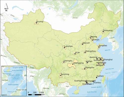
Table 1. The numbers of POI and POI pairs in each city

City	POI	All POI pairs N (m)	POI pairs sample size n
Shanghai	93842	4403.11356	9604
Dongguan	6682	22.321221	9600
Urumqi	3330	5.542785	9588
Lanzhou	2910	4.232595	9583
Beijing	25176	316.9029	9604
Nanjing	8403	35.301003	9602
Xiamen	3245	5.26339	9587
Tianjin	10698	57.218253	9603
Taiyuan	4877	11.890126	9597
Ningbo	5242	13.736661	9598
Guangzhou	13210	87.245445	9603
Chengdu	19399	188.150901	9604
Wuxi	7100	25.20145	9601
Kunming	5352	14.319276	9598
Hangzhou	14922	111.325581	9604
Wuhan	12960	83.97432	9603
Shantou	1894	1.792671	9553
Shenyang	5510	15.177295	9598
Shenzhen	12614	79.550191	9603
Suzhou	9975	49.745325	9603
Xi’an	9084	41.254986	9602
Zhengzhou	9479	44.920981	9602
Chongqing	12789	81.772866	9603
Changsha	6108	18.650778	9600
Qingdao	6670	22.241115	9600
Total	311471		239943

In each city, the sampling procedure includes three steps. First, according to Cochran’s sample size formula (n₀ = z²p(1-p)/e²), the sample size n₀ for infinite population is calculated with level of precision of 1% (e = 0.01) and confidence level of 95% (z = 1.96). Second, calculate the number of all possible origin-destination POI pairs in each city as population size N and derive sample size n for finite population by Cochran’s formula n = n₀ /(1+(n₀-1)/N) (Table 1). Third, ED and ND are calculated for each origin-destination pair. The EDs between the origin-destination pairs in each city are calculated based on the coordinate values in a Universal Transverse Mercator projection. Traditionally, the calculation of ND is based on network analysis using offline road network data (Lu, Charlton, and Fotheringham 2011; Lu et al. 2014; Morita, Suzuki, and Kei-ichi 2014). In this study, the NDs are approximated by the actual travel distances along the road networks because this is closer to how people utilize the road networks in reality and the results might be more effective for realistic applications. To enhance the efficiency and accuracy of the approximation, they are estimated online by using the routing service from Gaode Map. This service can return the travel distance (by walk or by car) between two locations. In most cases, the travel distance by car is used. However, when two locations are too close to each other, the actual travel distance will be overestimated by driving distance, because vehicles have to detour when they cannot enter small streets or pavements. Therefore, travel distance by walk is used if the walking duration is less than 15 minutes between two points. The 15-minute threshold is determined according to Weng et al. (2019). Otherwise, the travel distance by car is used. By this means, we have created a total of 239943 POI pairs for all selected cities (Table 1).

2.2. Detour index

Previous studies have revealed a significant proportional relationship between ND and ED (Wood, Clark, and Gatrell 2004). This relationship can be represented using ‘detour index’ (DI) (Gould 1970). For a given pair of origin and destination, DI is calculated as the ratio of ND to ED:

(1) $\mathrm{D}\mathrm{I}=\frac{\mathrm{N}\mathrm{D}}{\mathrm{E}\mathrm{D}}$(1)

At the city level, DI of a city indicates how much further on average a traveller must detour in this city, which reflects the average efficiency of road networks in a city. Following previous studies (Boscoe, Henry, and Zdeb 2012; Tamura, Koshizuka, and Ohsawa 2001), we estimate the city-level DI using a zero-intercept linear regression model:

(2) $y=\alpha x$(2)

where x and y are EDs and NDs of the observed origin-destination pairs, respectively. The slope α is the estimated city-level DI, which is solved using the ordinary least-squares method. We use the randomly sampled origin-destination pairs (see Section 2.1) to establish the linear regression models (with no intercept) for the 25 selected cities.

2.3. Functional data analysis

In addition to the measurement of city-level DI values, it is worth investigating how DI varies across scales in different cities. This is based on the method of FDA. Specifically, DI can be expressed as a function of ED, denoted as X_i(d), where X_i is the DI function for the ith city and d is ED. For the 25 selected cities, we establish their corresponding DI functions and investigate the modes of variation using the method of FDA.

In FDA, functional data are discrete observations at a finite number of points over a continuum (e.g. time and spatial location). In our case, functional data are the observations of the DI functions X_i(d) for each selected city i. The observations are made by collecting the DI values at various EDs of the sampled origin-destination pairs in each city. As FDA requires that observations on the subjects should be on the same domain, the first step is to make the observations comparable across subjects (e.g. across cities in our case) (Warmenhoven et al. 2019). Therefore, we first normalize the EDs of the sampled origin-destination pairs. This is made by grouping the original sampled origin-destination pairs in each city according to their EDs, and subsequently replacing d by group index r_j (j = 1, 2, …, N). The second step is to construct the DI functions X_i(r_j) for each city, which is based on the frequently used basis function fitting method. This method finds a consistent functional form that has the best fit to the observations for different cities, considering both the closeness to observations and the smoothness of functions. To separate amplitude variability and phase variability within the curves of DI functions, the third step is to align the functions constructed in the previous step. This is done by using the approach of warping. Finally, in the fourth step, we identify the modes of variability based on the approach of functional principal component analysis (FPCA). We explain the details of these four steps in the following sections. Steps two to four are implemented using the Matlab package: fdaM (http://www.psych.mcgill.ca/misc/fda/downloads/FDAfuns/Matlab/).

2.3.1. Normalizing EDs across cities

FDA requires that observations on the subjects should be on the same domain. However, for the 25 selected cities, they have different size and extent, resulting in different domains of observed EDs across cities (ranging from 100 m to 45 km). Therefore, before implementing FDA, we normalize the observed EDs of the sampled origin-destination pairs in each city based on the following procedures: First, in each city, the sampled origin-destination pairs are sorted ascendingly according to their EDs; Second, the sampled origin-destination pairs are divided into 100 groups by their ranks, denoted as r_j (j = 1, 2, …, N), with each group having equal number of point pairs; Third, for each group, the mean of its members’ DI values is used as the DI value of this group, denoted y_j. The subsequent FDA is, therefore, based on the normalized distance r_j and y_j.

2.3.2. Fitting DI values by basis functions

For each city, we fit the discrete observations using a basis expansion model as below:

(3) $y_j=X\left(r_j\right)+{\epsilon }_j$(3)

where ε_j is an error term with an expectation of zero. Function X(r) is of the following form:

(4) $X\left(r\right)=\sum _k^K{c}_k{\mathrm{\Phi }}_k\left(r\right)=c^{\mathbf{T}}\Phi$(4)

where the vector c contains K coefficients c_k that make X(r) a linear combination of the basis functions Ф_k(r). In other words, X(r) is the combination of K basis functions Ф_k(r). This leads to how to represent the basis functions Ф_k(r) and determine the number K. We adopt an order four B-spline basis system to represent our basis functions Ф_k(t), mainly because the B-spline basis functions are the most prevalent approximation system for non-periodic functional data (Ramsay and Silverman). To determine the function number K, we follow the approach used by Ramsay and Silverman (), which evaluates the effects of K according to an unbiased estimate of variance:

(5) $s^2=\frac{1}{N-K}\sum _j^N{\left(y_j-{\hat{y}}_j\right)}^2$(5)

The value of s² gradually declines when increasing the function number K, and a suitable value of K can be reached if s² becomes stable or no longer declined sharply (Ramsay and Silverman).

After the determination of the form and number of basis functions Ф_k(r), the next step is to estimate the coefficients c_k in Equation (4)(4) $X\left(r\right)=\sum _k^K{c}_k{\mathrm{\Phi }}_k\left(r\right)=c^{\mathbf{T}}\Phi$(4) . The estimation is carried out using an efficient smoothing method, i.e. the roughness penalty approach (Green and Silverman 1993), which estimates c_k by minimizing the penalized residual sum of squares:

(6) $c_k^{\ast }\mathrm{a}\mathrm{r}\mathrm{g}=\underset{c_k}{min}\left\{\parallel y_j-X\left(r_j\right){\parallel }^2+\lambda \int {\left[D^m{x}_i\left(r\right)\right]}^{2}dr\right\}$(6)

where $c_k^{\ast }$ refers to the estimation of c_k. D^m is the derivate of order m (m = 2 according to Ramsay (Ramsay and Silverman)), and λ is a smoothing parameter. Equation (6)(6) $c_k^{\ast }\mathrm{a}\mathrm{r}\mathrm{g}=\underset{c_k}{min}\left\{\parallel y_j-X\left(r_j\right){\parallel }^2+\lambda \int {\left[D^m{x}_i\left(r\right)\right]}^{2}dr\right\}$(6) consists of two parts. The first part ||y_{j –} X(r_j)||² measures the goodness of fit to the data. The second part, ${\int }^{{\left[D^m{X}_i\left(r\right)\right]}^2}dr$, is the roughness of the functions, multiplied by a smoothing parameter λ. The better the basis functions fit to the data, the smaller the first part is, but meanwhile the functions get rougher and may lead to the problem of overfitting. Therefore, a roughness penalty is used to balance the goodness of fit and the roughness of the basis functions. The larger the smoothing parameter λ is, the more the roughness of the basis functions is concerned (Ramsay and Silverman 2007). The determination of λ is based on the generalized cross-validation (GCV) criterion (Golub, Heath, and Wahba 1979), which can be expressed as:

(7) $\mathrm{G}\mathrm{C}\mathrm{V}\left(\lambda \right)=\left(\frac{N}{N-df\left(\lambda \right)}\right)\left(\frac{SSE}{N-df\left(\lambda \right)}\right)$(7)

where df is the degrees of freedom and SSE refers to the sum of squared errors. The smoothing parameter λ is automated chosen by minimizing the value of GCV(λ) using the grid-search optimization algorithm (Ramsay and Silverman).

2.3.3. Curves registration by a warping function

Warping is also referred to as continuous registration, which aims to map variant r to a registered r* (of the same domain) that makes each curve X(r*) closer to a datum curve X₀(r) (usually the mean curve). After the registration, the phase variation among all curves can substantially reduce while the amplitude variation becomes more explicit. As our data do not contain visible landmarks (e.g. minima, maxima or crossings of zero), we register our data by the continuous registration approach that uses the entire set of curves rather than their values at some specific landmarks (Ramsay, Hooker, and Graves 2009). Moreover, this approach offers the convenience of a fully automatic process.

The continuous registration approach finds a warping function h(r) that can map r to a registered r*. The warping function h(r) should satisfy the following constraints: (1) Strictly increasing; (2) Smooth; and (3) h(0) = 0 and h(R) = R, where [0, R] is the common interval of observations. After the registration, X(r*) should only differ from the datum curve X₀(r) in terms of amplitude (Ramsay, Hooker, and Graves 2009). If this is the case, and if principal component analysis is carried out on X(r*) and X₀(r), then the smallest eigenvalue should be near 0. Thus, we estimate the warping function h(r) by minimizing the smallest eigenvalue of C(h) (Ramsay, Hooker, and Graves 2009):

(8) $C\left(h\right)=\left[\begin{array}{cc}\int {\{X_0\left(r\right)\}}^{2}dr& \int X_0\left(r\right)X\left[h\left(r\right)\right]dr\\ \int X_0\left(r\right)X\left[h\left(r\right)\right]dr& \int {\{X_0\left[h\left(r\right)\right]\}}^{2}dr\end{array}\right]$(8)

2.3.4. Functional principal component analysis (FPCA)

FPCA is an extension of the ordinary PCA. For a better understanding of the implementation of FPCA, we briefly explain the ordinary PCA first before specifying the differences of FPCA. In PCA, the largest components of variation in the variables is identified by finding the weight vector β₁ = (β₁₁, …, β_p1)^T that maximizes the mean square $N^{-1}\sum _i{f}_{i1}^2$, where f_i1 is called Principal Component Scores, which can be expressed by the following equations:

(9) $f_{i1}=\sum _j{\beta }_{j1}{x}_{ij}={\beta }_1^{\mathrm{T}}{x}_i$(9)

(10) $\mathrm{s}.\mathrm{t}.\hspace{0.17em}\sum _j{\beta }_{j1}^2=\parallel {\beta }_1{\parallel }^2=1$(10)

Equation (10)(10) $\mathrm{s}.\mathrm{t}.\hspace{0.17em}\sum _j{\beta }_{j1}^2=\parallel {\beta }_1{\parallel }^2=1$(10) represents that the sum of squares of the weight vector β₁ should be one, otherwise $N^{-1}\sum _i{f}_{i1}^2$ would be made arbitrarily large. Subsequently, the next m largest variations in the variables can be found by calculating the new weight vectors β_m and the new scores f_im = β_m^Tx_i, which are again subject to the constrain || β_m ||² = 1 and the additional m-1 constraints:

(11) $\sum _j{\beta }_{jk}{\beta }_{jm}={{\beta }^{\prime }}_k{\beta }_m=0,(\mathrm{k}<\mathrm{m})$(11)

These constraints require that the newly calculated weights should be orthogonal to the previous identified ones, so that the information they reveal is not identical (Ramsay and Silverman).

For the functional version of PCA, the variables x and the weight vectors β are substituted by the functional values x(s) and the weight functions β(s), respectively. Thus, the Principal Component Scores f_i in the functional space are calculated as the integrations of variable s:

(12) $f_i=({\beta }_1,x_i)=\int {\beta }_1\left(s\right)x_i\left(s\right)ds$(12)

In this manner, the ordinary PCA is extended to FPCA, and similarly, the first step of FPCA is to identify the largest components of variation by finding a weight function β₁(s) that maximizes the mean squares of component scores

(13) $N^{-1}\sum _i{f}_{i1}^2$(13)

(14) $\mathrm{s}.\mathrm{t}.\parallel {\beta }_1{\parallel }^2=({\beta }_1,{\beta }_1)={\int }_1{\beta }^2\left(s\right)ds=1$(14)

In the subsequent steps, the remaining m largest variations are identified correspondingly by finding the weight functions that satisfy the orthogonality constraints (${\int }^{{\beta }_k}\left(s\right){\beta }_m\left(s\right)ds=0,k<m$) and calculating their component scores (Viviani, Gron, and Spitzer 2005). The weight functions β(s) are obtained by solving the following eigenequation with the largest eigenvalue $\xi$:

(15) $N^{-1}{X}^{T}X\beta =\xi \beta$(15)

After these procedures, a final step is to implement the varimax rotation (Kaiser 1958) on the first several components. Usually, the rotated components can provide more informative variability and hence outperform the original ones in terms of explaining variation across subjects (Ramsay and Silverman 2007).

3. Implementation and results

3.1. Characteristics of the city-level DI values

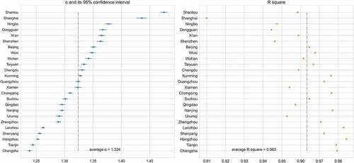
Figure 2 demonstrates the results of the linear regression of ND on ED for the 25 selected cities. The values of slope α (i.e. the city-level DI values) and R² of the 25 selected cities are summarized in Figure 3 (Table A1). The resulting DI values, as indicated by the coefficient α, range from 1.238 and 1.475 across cities with an average of 1.324. The R² ranges between 0.910 and 0.984, with an average of 0.963, indicating a significant linear relationship between ND and ED in all of the 25 selected cities.

Figure 2. Results of linear regression of network distance on Euclidean distance for the 25 cities

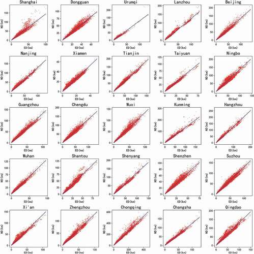
Figure 3. The regression coefficients, their 95 confidence intervals and R² of the 25 cities (ranked by α)

3.2. FPCA of the intra-city DI curves

3.2.1. Basis functions of each city

After distance normalization (see Section 2.3.1), the basis functions are fitted to the DI values in each of the 25 cities (see Section 2.3.2). In Figure 4, the red curves are order four B-spline basis functions and the blue dots are the DI values of the normalized distance groups. Each curve contains 15 splines, with the smoothing parameter λ = 0.1.

Figure 4. Basis functions fitted to intra-city DI (after normalization)

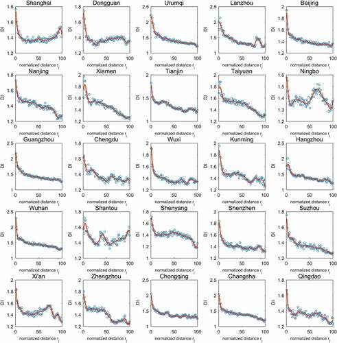
As illustrated by Figure 4, the fitted curves for most cities decline from the highest point in the short-distance groups to the long-distance groups. This suggests that the difference between ED and ND is greatest for nearby location point pairs and diminishes with ED increasing. However, the patterns of the fitted curves vary substantially from one city to another. Visual inspection reflects that there are three major modes of the fitted curves.

The first mode features the monotonous downward trend from the short distance groups with no or very small fluctuations. In this mode, the curves keep relatively stable through the middle- and long-distance groups. The fitted curves for cities such as Guangzhou, Wuhan, Chongqing and Beijing belong to this mode. Most of these cities have a low degree of polycentricity, as indicated by a previous study (Liu and Wang 2016), and this may affect travel patterns due to the spatial variation of street density (Engelfriet and Koomen 2018): A city with a low degree of polycentricity usually has much higher street density in its central areas and monotonously decline towards its suburban areas. Other cities such as Tianjin, Kunming and Chengdu have curves with similar patterns while containing small waves of fluctuations along the middle or long-distance groups.

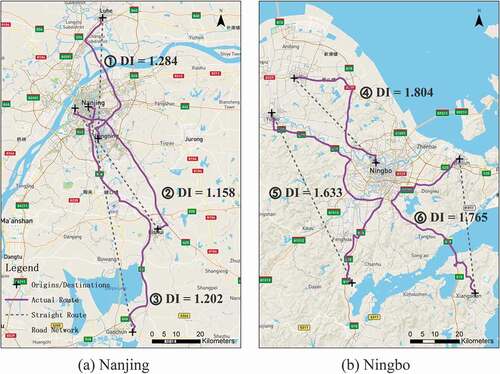
The second mode refers to fitted curves that saturate in the middle range distance groups. Examples of this mode include the fitted curves for Nanjing and Shenyang, which further decline after the saturation in the middle range distance groups. For Dongguan and Ningbo, however, their fitted curves even turn into an upward trend after saturation in the middle range distance groups. Cities in this ‘saturation’ mode have sub-centres that usually locates in the suburban areas far from the major centre. Physical conditions and structures of road networks that connect the major centre and the sub-centres may have an effect on long-distance travel. For the former cases (Nanjing as an example in Figure 5(a)), long-distance travels do not require much detour, probably because of the long and straight highways that stretch out from the major centre to sub-centres. In the latter cases (Ningbo as an example in Figure 5(b)), the upward trend is usually caused by complicated terrain conditions between sub-centres, including shorelines and mountainous areas.

Figure 5. Examples of long-distance travel routes in (a) Nanjing and (b) Ningbo

The third mode of fitted curves has erratic fluctuations along the entire range of distance groups. The curve for Shantou is of this mode, which generates multiple waves from the short distance groups to the long-distance groups. Cities in this mode contain city-wide physical barriers (e.g. mountainous area, bay, island) that separate the city into different parts and cause detours to medium or long-distance travel.

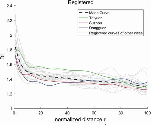
We then implemented curve registration by using a warping function (see Section 2.3.3). The resulting registered curves are shown in Figure 6, where the dashed curve refers to the mean curve. The mean curve effectively captures and reflects the general trend of variation of the DI values, which is a smooth downward trend with increasing ED between two location points. The resulting registered curves were then used for FPCA, which further determines the modes of variations latent in the functional observations.

Figure 6. The registered DI curves, with the dash curve representing the mean curve. The registered DI curves for several representative cities are highlighted

3.2.2. Rotated functional principal components (FPCs) and their scores

By applying FPCA and Varimax-rotation mentioned in Section 2.3.4, we obtain the first three of the rotated FPCs (Figure 7(d)) and their effects on the mean curve (Figure 7(a–c)). The blue curves are the mean DI curves, and the green and red curves show the effects of adding/subtracting a suitable multiple of each of the three FPCs to the mean. The first three FPCs collectively capture 94% of the variability of the DI functions in the 25 cities. The greatest variability (43%) is observed in the left part (‘heads’) of the DI curves, which has been explained by the FPC1. The following are the variations at the curves’ ‘bodies’ and ‘tails’, which have been captured by the second (31%) and the third (20%) FPCs, respectively.

Figure 7. Varimax-rotated Functional Principal Components of variation in 25 cities’ DI curves. The amount of variation accounted for is at the top of each figure. Curves in (d) are the three harmonics (FPCs). In (a), (b) and (c), the blue curves are the mean DI curves, and the green and red curves show the effects of adding and subtracting a multiple of the FPCs to the mean

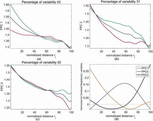
FPC1 captures the variation at the ‘heads’ of the DI curves. It is positive with large absolute value before r_j = 40, and makes this part of the DI curves deviate from the mean curve. FPC1 changes to a small negative value from r_j = 50 to r_j = 90, and hence has an inverting effect on this part of the curves. FPC2 mainly explains the difference in the curve shape among cities. It is a large positive value in the middle part of the curves, and becomes small negative values at the two ends. Therefore, cities with a high score of FPC2 have DI values larger than the mean in the middle-distance range, and smaller than the mean at both ends. Compared to FPC1, FPC3 emphasizes the variations at the tail parts of the DI curves. FPC3 is small and negative before r_j = 60 but then rises into positive values afterwards. The score of FPC3 determines how much the tails parts of the DI curves deviate from the mean curve.

To examine to what extent each FPC affects each city’s DI curve, we calculated the FPC scores for the 25 cities (See Equation (9))(9) $f_{i1}=\sum _j{\beta }_{j1}{x}_{ij}={\beta }_1^{\mathrm{T}}{x}_i$(9) and projected the results on the planes (with the FPC scores as axes (Figure 8)). For each city, the value of each FPC score is the exact multiple by which this FPC adds to or subtracts from the mean curve. Since all FPC scores are non-zero, it is evident that the shape of the DI curve (Figure 5) is the result of the joint effects of these three FPCs (Figure 7). The corresponding contribution of each FPC to shape the DI curves of different cities is shown in Figure 8. For a better understanding, we select Taiyuan, Suzhou and Dongguan as three representative examples to describe the joint effects of FPCs.

Figure 8. Scatter plot of varimax-rotated FPC scores in components’ space. Score of FPC2 mainly affects the overall shape of the DI curve. FPC1 and FPC3 scores affect the variations of the head and the tail parts of DI curves, which represents short-distance and long-distance travel respectively

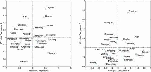
As shown in Figure 8, Taiyuan is at the top right quadrant of the left plane, indicating that Taiyuan has high scores of FPC1 and FPC2. Since FPC1, FPC2 and FPC3 correspondingly affect the variations at the head, the middle and the tail parts of DI curves (Figure 7), high positive scores for FPC1 and 2 result in a DI curve that varies substantially from the mean curve from the head to the main body of the DI curve, which is the case for Taiyuan. As shown by Figure 6, the entire DI curve of Taiyuan deviates far above the mean curve until the tail. However, Suzhou is an opposite case. In Figure 8, Suzhou locates at the bottom left quadrant of both planes, indicating that all the three FPC scores are negative. This suggests that for Suzhou, the DI values are small in the whole distance range, probably due to its dense and regular road network in this city. Dongguan represents another case. Figure 8 shows that the FPC1 and FPC2 scores of Dongguan are negative while its FPC3 score is positive. Such an FPC combination leads to a DI curve with a ‘head’ below and a ‘tail’ above the mean curve, and a middle part close to the mean curve (Figure 6).

4. Discussion

4.1. Comparison with previous studies

In general, our city-level results are consistent with those reported by previous literature, although some differences exist. The average DI (1.324) obtained in our study is slightly larger than that of the Japanese cities (1.3035), as reported by Morita, Suzuki, and Kei-ichi (2014). Additionally, ten cities in Japan have DI over 1.5, but in our study, the largest DI is less than 1.48. Compared to the country-level DI of the USA (1.417) estimated by Boscoe, Henry, and Zdeb (2012), the DI values in our study are smaller (1.238–1.475), probably due to the denser road networks in Chinese cities.

We also compared our results with the simulation of a null model developed by Dong et al. (2016), in which they simulated a monocentric city with Manhattan grids road network (ND between (0,0) and (x,y) is |x|+|y|). By assuming a uniform distribution of population, they calculated the ND and ED from randomly generated points to the network centre. They further used the population-weighted efficiency, which is the weighted sum of the reciprocal of the DI, to quantify the relationships between ND and ED. Their simulation yielded a result of 0.77, which is equivalent to a DI value of 1.2987. However, in our study, most cities (20 out of 25) have DI values greater than 1.2987. Probable reasons are as follows: (1) Most of these cities are not monocentric. (2) The actual distribution of the population is not uniform in most cases. Instead, they usually concentrate in certain specific residential areas in these cities. (3) Terrain conditions are usually complicated in the real world, so that the network structures are also more complicated and thus less efficient than those simulated by the null model.

4.2. Effectiveness of the estimated DI

Since distance is essential to many types of spatial analysis, our results have demonstrated that using ED may cause bias in realistic cases. In methods involving search radius, using ED affects the results by overestimating the search area. For instance, according to the estimated average DI in our study (1.324), the search area of KDE as well as the service area of public facilities will be overestimated by 1.753 times (square of DI) if ED is used.

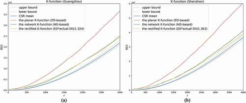
To test whether the estimated DI can be used as an effective and convenient method to produce realistic results, we took Ripley’s K-function analysis (Ripley 1976) as an example to carry out comparative experiments using ED, DI-corrected ED and ND. We collected POIs of primary schools in the central districts of Guangzhou and Shenzhen and applied K-function to the point patterns. The K-functions were calculated in three different modes: (1) the planar K-function (ED-based), (2) the network K-function (ND-based), and (3) the rectified K-function (planar K-function with ED multiplied by the DI). Since the observed and Monte-Carlo simulated K-functions are biased in the same manner due to the edge effect (Smith 2011), no edge correction is applied in our experiments.

As illustrated in Figure 9, in both cases of Guangzhou and Shenzhen, the planar K-functions (ED-based) largely overestimated the clustering patterns of primary schools, as compared with those yielded by the network K-functions (ND-based). This is in line with findings in previous literature (Yamada and Thill 2004). Not surprisingly, this bias can be substantially reduced by applying the estimated DI to ED. After multiplying ED by the city-level DI, the curves of the corrected planar K-functions (ED-based) move significantly towards those of the network K-functions (ND-based). Similar corrections can also be made to other spatial analysis methods using the estimated DI. Although ND is generally more reasonable for realistic cases, acquiring ND is not always an easy task (as described in Section 1). Compared with the use of actual ND, this approach can ensure the accuracy of analysis results while requiring substantially lower computation costs and data acquisition costs.

Figure 9. Comparison of K-functions using three different distance metrics

Another issue is that for cities with no empirical results of DI, how to estimate an appropriate DI for the correction of ED. Based on an additional experiment, we found that the city-level DI is significantly correlated with the mean Euclidean distance of urban patches. The distance of urban patches refers to the distance between the centroids of two urban patches. Urban patches can be obtained by interpretating satellite images (Yu et al. 2014) or from open sources, for example, Global Human Settlement Layer (Florczyk et al. 2019) and the MODIS 500-m map of global urban extent (Schneider, Friedl, and Potere 2010). In this experiment, urban patches (100-m resolution) for all 25 cities were collected from https://essd.copernicus.org/preprints/essd-2019-65/ (Kuang et al. 2021). For each city, the average distance of urban patch centroids was calculated as the mean Euclidean distance of urban patches. As shown by Figure 10(a), the results of linear regression analysis suggest a significant relationship between the city-level DI and the mean Euclidean distance of urban patches. Therefore, one can predict the DI value by using the mean Euclidean distance of urban patches if a city’s DI is unknown.

Figure 10. (a) Significant relationship between the city-level DI and the mean Euclidean distance of urban patches. Chongqing is an outlier and thus is removed from the linear regression analysis. (b) Comparison of K-functions using ED, ND, and corrected ED based on the actual and predicted DI values

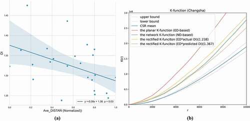
We then evaluate the accuracy of DI prediction based on the k-nearest neighbour (kNN) regression with a single variable of mean Euclidean distance of urban patches. kNN is an intuitive and efficient classification method in pattern recognition. An object is classified by a voting of its neighbours in the feature space. The object is assigned the most common class among its k nearest neighbours. kNN regression is used for estimating continuous variables according to similar rules. In kNN regression, the voting result is the average (or weighted average) of the property values of its k nearest neighbours (Altman 1992). Leave-one-out cross-validation was used to evaluate the performance of the kNN regression. After multiple experiments, k = 10 yielded the most accurate result (see Table A2 for full results). The Mean Absolute Difference is 0.042 and the Mean Absolute Percent Error is 3.123%. To evaluate the impacts of the DI prediction errors, we selected the city with a large error (i.e. Changsha), and compared its K-function outcomes using both the actual and predicted DI. As shown in Figure 10(b), K-function using the predicted DI also reduces most of the bias (overestimation of the clustering patterns) caused by the planar K-function (ED-based) just as the network K-function (ND-based) does.

Distance is also one of the key parameters defining the spatial weight matrix for many methods such as GWR. Using a biased distance will affect the definition of neighbourhood configuration, as pointed out by Shahid et al. (2009) who had compared the usage of Euclidean distance and Minkowski distance in spatial regression models. Lu et al. (2014) has also come into similar conclusions by 720 GWR models based on different distance metrics (including ED, ND and Travel Time).

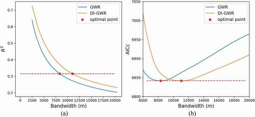
To illustrate how DI works for GWR, we compared the conventional GWR model and a DI-rectified GWR model (DI-GWR) on population prediction. The models predict the census level population by night-time light. The population data is the 2010 census data of Guangzhou. The night-time light is the Visible and Infrared Imaging Suite (VIIRS) Day Night Band (DNB) on board of JPSS satellites. Yearly data of the year 2012 is used as the independent variable (downloaded from the Earth Observation Group: https://eogdata.mines.edu/products/vnl/). A number of models built upon different bandwidths are compared based on two commonly used model goodness-of-fit diagnostic, i.e. the corrected Akaike information criterion (AICc) and R². Figure 11 indicates that for any fixed bandwidth after the AICc lines converge in Figure (b), a DI-GWR model always has the smaller AICc and higher R² than the conventional one. However, when the bandwidth of a GWR model is optimized automatically based on criteria of AICc, they reach the same optimal points even though the bandwidths of these two models with bandwidths are different. This is reasonable because the GWR model rectified by a global DI is a linearly stretched version of itself by its nature. Therefore, the spatial heterogeneity of the DI is taken into consideration and will be discussed in the next section.

Figure 11. Comparison of AICc and R² between the conventional GWR model and the DI-GWR model

4.3. The spatial heterogeneity of the DI

As the variations of DI might be caused by the difference in road density, polycentricity, physical barriers (e.g. mountainous areas, bays, islands, etc.), Guangzhou is taken as an example to illustrate the spatial heterogeneity of the DI.

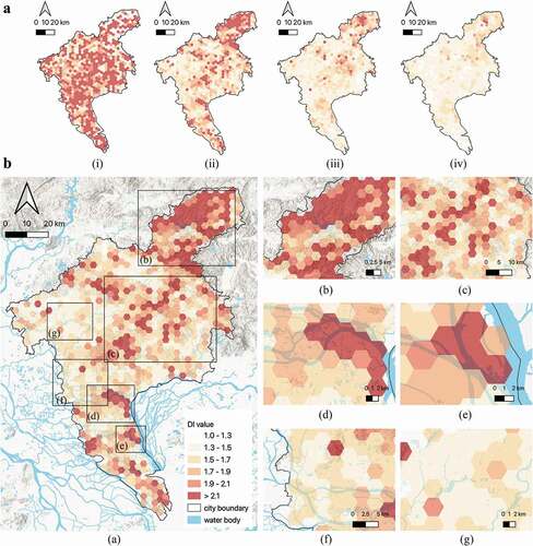
Generally, the DI declines from the short-distance groups to the long-distance groups, as concluded from Section 3.2. Figure 12A is also telling the same story by demonstrating local DI values of different distance groups: (i) indicates that in most areas in Guangzhou, travelling to somewhere within 3 km will end up with a detour of about two times the straight-line distance. In longer distance groups (ii), (iii) and (iv), the DI values further decline in most areas except some mountainous areas or water-barriered areas. Figure 12B has highlighted some areas with large or small DI values as examples: Mountainous areas and areas with rivers or islands lead to large DI (a-e), while urban areas with dense and regular road networks lead to small DI (f-g).

Figure 12. A. Local DI in different distance groups. The DI value in each hexagon cell (radius of 1.5 km) is averaged by 30 O-D pairs originating from the centroid of the cell and ending at a random Gaode POI within a specific distance interval: (i) Within 3 km. (ii) 3 to 10 km. (iii) 10 to 30 km. (iv) 30 to 50 km. B. The spatial heterogeneity of the DI. (a) is an enlarged version of (ii) in Panel A. (b-c) are mountainous areas with large DI. (d-e) are areas with large DI caused by rivers and islands. (f) and (g) are city centre and sub-centre with small DI

5. Conclusion and future work

This study investigates the quantitative relationships between straight-line ED and ND. In the 25 selected Chinese cities, we estimated the DI, i.e. the ratio of ND to ED, at the city level and analysed their variations at the intra-city level. The results can help improve the accuracy of spatial analysis methods when they have no ‘network version’ or when road network data is unavailable.

At the city level, we found that in Chinese cities, ND and ED are highly correlated. The city-level DI values of the 25 selected cities range from 1.238 to 1.475 with an average of 1.324. At the intra-city scale, the results of the FDA demonstrate the general modes of the fitted curves. The DI declines from the short-distance groups to the long-distance groups, suggesting that the difference between ED and ND is larger for nearby location point pairs and diminishes with increasing ED. Although this declining trend seems intuitive because longer trips may take advantage of long stretches of straight routes, our study modelled and verified this trend using the real-world data. We also captured the variations among cities and identified three different variation modes, which are the monotonous-downward mode, the saturation mode and the fluctuation mode. By applying FPCA and varimax rotation on the fitted DI curves, the resulting first three FPC can explain 94% of the variability all together. The variations explained by FPC1 (43%) are observed mainly in the short-distance part (‘head’) of the DI curves. FPC2 (31%) and FPC3 (20%) capture the variations at the curves’ ‘bodies’ and ‘tails’, in other words, the variations of middle-distance and long-distance travel. The 25 cities are then projected to the principal component plane according to their FPC scores.

These results are useful for applications of spatial analysis with limited computing resources or insufficient network data. The experiments in section 4.2 demonstrate that spatial analysis methods using ED adjusted by DI can produce similar results to its ND version. We also demonstrated that the DI is negatively dependent on the mean distance of urban patches, which can be used as an indicator to predict the DI for cities with no empirical results of DI. We developed a DI prediction based on kNN, which can yield predicted DI with the mean error of less than 4%.

Our study suffers from several limitations, pointing to potential directions for future research. First, we used the walking mode and the driving mode when estimating the NDs by online routing service. However, walking through tunnels or along the motorways is not allowed, while in the driving mode, road restrictions (e.g. one-way street) would also lead to some bias. In future work, this issue can be addressed by using an improved API that allows the setting of mixed travel modes. Second, when considering the spatial heterogeneity of the DI, uncertainty induced by the definition of spatial unit (e.g. modifiable areal unit problem) might affect the results. In further research, experiments on the spatial heterogeneity will be carried out in more cities after the uncertainty is further evaluated.

Disclosure statement

No potential conflict of interest was reported by the authors.

Additional information

Funding

This work was supported by the National Natural Science Foundation of China [41871306]; National Key R&D Program of China [2019YFA0607201]; Fundamental Research Funds for the Central Universities [20lgzd09]; Guangdong Natural Science Funds for Distinguished Young Scholar [2021B1515020104]; Open Fund of Key Laboratory of Geographic Information Science (Ministry of Education), East China Normal University [KLGIS2020A02].

Appendix

Table A1 The regression coefficients and their 95 confidence intervals or the 25 cities

City	α and its 95% confidence interval	R^2
Shanghai	1.436 ± 0.009	0.910
Dongguan	1.367 ± 0.007	0.944
Urumqi	1.29 ± 0.005	0.953
Lanzhou	1.262 ± 0.003	0.983
Beijing	1.351 ± 0.005	0.965
Nanjing	1.295 ± 0.004	0.977
Xiamen	1.323 ± 0.005	0.954
Tianjin	1.244 ± 0.004	0.979
Taiyuan	1.334 ± 0.005	0.967
Ningbo	1.377 ± 0.006	0.947
Guangzhou	1.324 ± 0.004	0.973
Chengdu	1.331 ± 0.005	0.959
Wuxi	1.348 ± 0.005	0.968
Kunming	1.328 ± 0.004	0.976
Hangzhou	1.253 ± 0.003	0.984
Wuhan	1.342 ± 0.005	0.961
Shantou	1.475 ± 0.006	0.958
Shenyang	1.256 ± 0.004	0.972
Shenzhen	1.363 ± 0.006	0.946
Suzhou	1.301 ± 0.005	0.965
Xi’an	1.365 ± 0.005	0.959
Zhengzhou	1.289 ± 0.004	0.971
Chongqing	1.31 ± 0.004	0.976
Changsha	1.238 ± 0.003	0.979
Qingdao	1.295 ± 0.005	0.957
Average	1.324	–

Table A2. kNN results of DI prediction (k = 10)

City	Mean Distance of urban patches	DI	Predicted DI	Absolute Difference	Absolute Percent Error(%)
Beijing	50318.63	1.351	1.297	0.054	3.963
Changsha	37428.52	1.238	1.344	0.106	8.592
Chengdu	45215.61	1.331	1.330	0.000	0.036
Dongguan	148032.6	1.367	1.348	0.019	1.424
Guangzhou	31475.43	1.324	1.336	0.012	0.902
Hangzhou	39785.22	1.253	1.307	0.054	4.339
Kunming	51087.51	1.328	1.349	0.022	1.637
Lanzhou	25511.72	1.262	1.306	0.044	3.511
Nanjing	50877.73	1.295	1.313	0.018	1.383
Ningbo	48230.2	1.377	1.305	0.072	5.233
Qingdao	47946.98	1.295	1.299	0.004	0.304
Shanghai	59651.22	1.436	1.325	0.111	7.755
Shantou	39793.3	1.475	1.335	0.140	9.522
Shenyang	23324.88	1.256	1.303	0.047	3.772
Shenzhen	55947.14	1.363	1.346	0.018	1.292
Suzhou	20716.5	1.301	1.302	0.001	0.086
Taiyuan	51203.13	1.334	1.351	0.017	1.285
Tianjin	32750.55	1.244	1.305	0.061	4.864
Urumqi	56604.87	1.290	1.353	0.063	4.851
Wuhan	25746.46	1.342	1.347	0.005	0.383
Wuxi	34090.55	1.348	1.327	0.021	1.590
Xiamen	42939.71	1.323	1.350	0.027	2.027
Xi’an	16069.96	1.365	1.296	0.069	5.081
Zhengzhou	50934.21	1.289	1.304	0.014	1.116
Average	45425.09	1.324	1.324	0.042	3.123

Table A3. Ten repeated experiments of Cochran’s sampling (Changsha and Dongguan as examples)

City	Exp. No.	DI	City	Exp. No.	DI
Changsha	1	1.271	Dongguan	1	1.433
	2	1.282		2	1.419
	3	1.264		3	1.398
	4	1.246		4	1.365
	5	1.238		5	1.352
	6	1.234		6	1.366
	7	1.238		7	1.383
	8	1.239		8	1.391
	9	1.264		9	1.409
	10	1.238		10	1.367
	Average	1.251		Average	1.388
	Stdev	0.017		Stdev	0.026
	Std/Ave	1.382%		Std/Ave	1.909%

References

- Altman, N. S. 1992. “An Introduction to Kernel and Nearest-neighbor Nonparametric Regression.” The American Statistician 46 (3): 175–185.
- Apparicio, P., M. Abdelmajid, M. Riva, and R. Shearmur. 2008. “Comparing Alternative Approaches to Measuring the Geographical Accessibility of Urban Health Services: Distance Types and Aggregation-error Issues.” International Journal of Health Geographics 7 (1): 7. doi:https://doi.org/10.1186/1476-072X-7-7.
- Boscoe, F. P., K. A. Henry, and M. S. Zdeb. 2012. “A Nationwide Comparison of Driving Distance versus Straight-Line Distance to Hospitals.” Professional Geographer 64 (2). doi:https://doi.org/10.1080/00330124.2011.583586.
- Buczkowska, S., N. Coulombel, and M. de Lapparent. 2019. “A Comparison of Euclidean Distance, Travel Times, and Network Distances in Location Choice Mixture Models.” Networks and Spatial Economics 19 (4): 1215–1248. doi:https://doi.org/10.1007/s11067-018-9439-5.
- Buhl, J., K. Hicks, E. R. Miller, S. Persey, O. Alinvi, and D. J. T. Sumpter. 2008. “Shape and Efficiency of Wood Ant Foraging Networks.” Behavioral Ecology and Sociobiology 63 (3): 451–460. doi:https://doi.org/10.1007/s00265-008-0680-7.
- Chen, Y., X. Chen, Z. Liu, and X. Li. 2020. “Understanding the Spatial Organization of Urban Functions Based on Co-location Patterns Mining: A Comparative Analysis for 25 Chinese Cities.” Cities 97: 102563. doi:https://doi.org/10.1016/j.cities.2019.102563.
- Cochran, W. Sampling techniques (3rd ed.). New York :: Wiley. 2007.https://glad.geog.umd.edu/Potapov/_Library/Cochran_1977_Sampling_Techniques_Third_Edition.pdf
- Dong, J. J., L. Wang, J. Gill, and J. Cao. 2018. “Functional Principal Component Analysis of Glomerular Filtration Rate Curves after Kidney Transplant.” Statistical Methods in Medical Research 27 (12): 3785–3796. doi:https://doi.org/10.1177/0962280217712088.
- Dong, L., R. Li, J. Zhang, and Z. Di. 2016. “Population-weighted Efficiency in Transportation Networks.” Scientific Reports 6: 26377. doi:https://doi.org/10.1038/srep26377.
- Eldridge, J. D., and J. P. Jones III. 1991. “Warped Space: A Geography of Distance Decay.” The Professional Geographer 43 (4): 500–511. doi:https://doi.org/10.1111/j.0033-0124.1991.00500.x.
- Engelfriet, L., and E. Koomen. 2018. “The Impact of Urban Form on Commuting in Large Chinese Cities.” Transportation 45 (5): 1269–1295. doi:https://doi.org/10.1007/s11116-017-9762-6.
- Florczyk, A. J., C. Corbane, D. Ehrlich, S. Freire, T. Kemper, L. Maffenini, … M. Schiavina. 2019. “GHSL Data Package 2019.” Luxembourg, EUR 29788 (10.2760): 290498.
- Fraiman, R., A. Justel, R. Liu, and P. Llop. 2014. “Detecting Trends in Time Series of Functional Data: A Study of Antarctic Climate Change.” Canadian Journal of Statistics 42 (4): 597–609. doi:https://doi.org/10.1002/cjs.11231.
- Gastner, M. T., and M. E. Newman. 2006. “Shape and Efficiency in Spatial Distribution Networks.” Journal of Statistical Mechanics: Theory and Experiment 2006 (1): P01015. doi:https://doi.org/10.1088/1742-5468/2006/01/P01015.
- Girres, J. F., and G. Touya. 2010. “Quality Assessment of the French OpenStreetMap Dataset.” Transactions in GIS 14 (4): 435–459. doi:https://doi.org/10.1111/j.1467-9671.2010.01203.x.
- Golub, G. H., M. Heath, and G. Wahba. 1979. “Generalized Cross-validation as a Method for Choosing a Good Ridge Parameter.” Technometrics 21 (2): 215–223. doi:https://doi.org/10.1080/00401706.1979.10489751.
- Gould, P. 1970. “Quantitative Geography: Cole, JP and CAM King (1968): London: John Wiley and Sons Ltd. 95s Cloth, 55s Paper.” Geoforum 1 (1): 101–102. doi:https://doi.org/10.1016/0016-7185(70)90018-7.
- Green, P. J., and B. W. Silverman. 1993. Nonparametric Regression and Generalized Linear Models: A Roughness Penalty Approach. London :: Chapman and Hall/CRC.
- Jokar Arsanjani, J., and M. Bakillah. 2015. “Understanding the Potential Relationship between the Socio-economic Variables and Contributions to OpenStreetMap.” International Journal of Digital Earth 8 (11): 861–876. doi:https://doi.org/10.1080/17538947.2014.951081.
- Kaiser, H. F. 1958. “The Varimax Criterion for Analytic Rotation in Factor Analysis.” Psychometrika 23 (3): 187–200. doi:https://doi.org/10.1007/BF02289233.
- Karduni, A., A. Kermanshah, and S. Derrible. 2016. “A Protocol to Convert Spatial Polyline Data to Network Formats and Applications to World Urban Road Networks.” Scientific Data 3 (1): 1–7. doi:https://doi.org/10.1038/sdata.2016.46.
- Kuang, W., Zhang, S., Li, X., & Lu, D. (2021). A 30 m resolution dataset of China's urban impervious surface area and green space, 2000–2018. Earth System Science Data, 13(1), 63–82. doi:https://doi.org/10.5194/essd-13-63-2021
- Liu, X., and M. Wang. 2016. “How Polycentric Is Urban China and Why? A Case Study of 318 Cities.” Landscape and Urban Planning 151: 10–20. doi:https://doi.org/10.1016/j.landurbplan.2016.03.007.
- Lu, B. B., M. Charlton, and A. S. Fotheringham. 2011. “Geographically Weighted Regression Using a Non-Euclidean Distance Metric with a Study on London House Price Data.” Spatial Statistics 2011: Mapping Global Change 7: 92–97. doi:https://doi.org/10.1016/j.proenv.2011.07.017.
- Lu, B. B., M. Charlton, P. Harris, and A. S. Fotheringham. 2014. “Geographically Weighted Regression with a Non- Euclidean Distance Metric: A Case Study Using Hedonic House Price Data.” International Journal of Geographical Information Science 28 (4): 660–681. doi:https://doi.org/10.1080/13658816.2013.865739.
- Lv, M., J. E. Fowler, and L. Jing. 2019. “Spatial Functional Data Analysis for the Spatial–Spectral Classification of Hyperspectral Imagery.” IEEE Geoscience and Remote Sensing Letters 16 (6): 942–946. doi:https://doi.org/10.1109/lgrs.2018.2884077.
- Miller, H. J., and E. A. Wentz. 2003. “Representation and Spatial Analysis in Geographic Information Systems.” Annals of the Association of American Geographers 93 (3): 574–594. doi:https://doi.org/10.1111/1467-8306.9303004.
- Morita, M., K. Suzuki, and O. Kei-ichi. 2014. “An Empirical Study of the Ratio of the Road Distance to the Straight Line Distance in Major Cities in Japan.” Theory and Applications of GIS 22 (1): 1–7. doi:https://doi.org/10.5638/thagis.22.1.
- Nicoară, M., and I. Haidu. 2011. “Creation of the Roads Network as a Network Dataset within a Geodatabase.” Geographia Technica 6: 81–86.
- Okabe, A., K. I. Okunuki, and S. Shiode. 2006. “The SANET Toolbox: New Methods for Network Spatial Analysis.” Transactions in GIS 10 (4): 535–550. doi:https://doi.org/10.1111/j.1467-9671.2006.01011.x.
- Ramsay, J. O., and B. W. Silverman. 2007. Applied Functional Data Analysis: Methods and Case Studies.New York :: Springer.
- Ramsay, J. O., G. Hooker, and S. Graves. 2009. Functional Data Analysis with R and MATLAB. New York :: Springer.
- Ripley, B. D. 1976. “The Second-order Analysis of Stationary Point Processes.” Journal of Applied Probability 13 (2): 255–266. doi:https://doi.org/10.2307/3212829.
- Rossi, N., X. Wang, and J. O. Ramsay. 2002. “Nonparametric Item Response Function Estimates with the EM Algorithm.” Journal of Educational and Behavioral Statistics 27 (3): 291–317. doi:https://doi.org/10.3102/10769986027003291.
- Schneider, A., M. Friedl, and D. Potere. 2010. “Monitoring Urban Areas Globally Using MODIS 500 M Data: New Methods and Datasets Based on Urban Ecoregions.” Remote Sensing of Environment 114 (8): 1733–1746. doi:https://doi.org/10.1016/j.rse.2010.03.003.
- Shahid, R., S. Bertazzon, M. L. Knudtson, and W. A. Ghali. 2009. “Comparison of Distance Measures in Spatial Analytical Modeling for Health Service Planning.” BMC Health Services Research 9 (1): 1–14. doi:https://doi.org/10.1186/1472-6963-9-200.
- Smith, T. E. 2011. “4_K_Functions.” 4_K_Functions. Notebook for spatial data analysis. https://www.seas.upenn.edu/~ese502/NOTEBOOK/Part_I/4_K_Functions.pdf
- Su, S., C. Lei, A. Li, J. Pi, and Z. Cai. 2017. “Coverage Inequality and Quality of Volunteered Geographic Features in Chinese Cities: Analyzing the Associated Local Characteristics Using Geographically Weighted Regression.” Applied Geography 78: 78–93. doi:https://doi.org/10.1016/j.apgeog.2016.11.002.
- Tamura, K., T. Koshizuka, and Y. Ohsawa. 2001. “Relationship between Road Distance and Euclidean Distance on Road Networks.” Papers on City Planning 36: 877–882. (In Japanese). https://ci.nii.ac.jp/naid/10007466237/en/
- Tobler, W. R. 1970. “A Computer Movie Simulating Urban Growth in the Detroit Region.” Economic Geography 46 (sup1): 234–240. doi:https://doi.org/10.2307/143141.
- Ullah, S., and C. F. Finch. 2013. “Applications of Functional Data Analysis: A Systematic Review.” BMC Medical Research Methodology 13 (1): 43. doi:https://doi.org/10.1186/1471-2288-13-43.
- Viviani, R., G. Gron, and M. Spitzer. 2005. “Functional Principal Component Analysis of fMRI Data.” Human Brain Mapping 24 (2): 109–129. doi:https://doi.org/10.1002/hbm.20074.
- Wang, F., and Y. Xu. 2011. “Estimating O–D Travel Time Matrix by Google Maps API: Implementation, Advantages, and Implications.” Annals of GIS 17 (4): 199–209. doi:https://doi.org/10.1080/19475683.2011.625977.
- Warmenhoven, J., S. Cobley, C. Draper, A. Harrison, N. Bargary, and R. Smith. 2019. “Considerations for the Use of Functional Principal Components Analysis in Sports Biomechanics: Examples from On-water Rowing.” Sports Biomechanics 18 (3): 317–341. doi:https://doi.org/10.1080/14763141.2017.1392594.
- Weng, M., N. Ding, J. Li, X. Jin, H. Xiao, Z. He, and S. Su. 2019. “The 15-minute Walkable Neighborhoods: Measurement, Social Inequalities and Implications for Building Healthy Communities in Urban China.” Journal of Transport & Health 13: 259–273. doi:https://doi.org/10.1016/j.jth.2019.05.005.
- Wood, D. J., D. Clark, and A. C. Gatrell. 2004. “Equity of Access to Adult Hospice Inpatient Care within North-west England.” Palliative Medicine 18 (6): 543–549. doi:https://doi.org/10.1191/0269216304pm892oa.
- Yamada, I., and J.-C. Thill. 2004. “Comparison of Planar and Network K-functions in Traffic Accident Analysis.” Journal of Transport Geography 12 (2): 149–158. doi:https://doi.org/10.1016/j.jtrangeo.2003.10.006.
- Yazdani, A., and P. Jeffrey. 2011. “Complex Network Analysis of Water Distribution Systems.” Chaos: An Interdisciplinary Journal of Nonlinear Science 21 (1): 016111. doi:https://doi.org/10.1063/1.3540339.
- Yu, B., S. Shu, H. Liu, W. Song, J. Wu, L. Wang, and Z. Chen. 2014. “Object-based Spatial Cluster Analysis of Urban Landscape Pattern Using Nighttime Light Satellite Images: A Case Study of China.” International Journal of Geographical Information Science 28 (11): 2328–2355. doi:https://doi.org/10.1080/13658816.2014.922186.
- Zou, H., Y. Yue, Q. Li, and A. G. O. Yeh. 2012. “An Improved Distance Metric for the Interpolation of Link-based Traffic Data Using Kriging: A Case Study of a Large-scale Urban Road Network.” International Journal of Geographical Information Science 26 (4): 667–689. doi:https://doi.org/10.1080/13658816.2011.609488.