The Moran Spectrum as a Geoinformatic Tupu: implications for the First Law of Geography

ABSTRACT

Geoinformatic Tupu, or Geoinformatic graph spectrum, is a theoretical as well as a technical framework for generalizing geographic knowledge and solving real world problems. Geoinformatic Tupu is a promising platform for capitalizing on the technical advances of Geographic Information Systems, and to integrate the Chinese traditional way of thinking with modern information technology. It has been one of the major research topics in the Chinese GIScience community in recent decades, with an evolving epistemological development. A core objective of Geoinformatic Tupu is to recover and represent geographic principles with the Tupu approach, which is adopted in this paper to formulate the First Law of Geography (FLG) [i.e. the law of spatial autocorrelation] as the Moran Spectrum – a combination of sequential diagrams, graphs, and numeric components. Using the Moran Spectrum as a conduit, we present the theory of Moran Eigenvector Spatial Filtering (MESF), a distinct branch of spatial statistics that has demonstrable advantages in statistical modelling and machine learning, but has yet to be widely disseminated due to its conceptual and computational complexity. This paper demonstrates the effectiveness of the Tupu approach in enriching the representation of the FLG as well as deepening its applications. It also suggests inclusion of the Moran Spectrum as a core component in Geoinformatic Tupu.

KEYWORDS:

• Geoinformatic Tupu
• Moran Spectrum
• spatial autocorrelation
• Moran Eigenvector Spatial Filtering

Introduction

Geoinformatic Tupu is a familiar term in the GIScience community in China, although it may be unheard of elsewhere. Tupu is a compound word in Chinese, constituting two characters Tu (graph) and Pu (sequence, spectrum). A Tupu stands for a sequence or spectrum of a graph. A Geoinformatic Tupu therefore could be taken to mean literally a sequence of maps. As the name of a theoretical and technical framework, Geoinformatic Tupu has rich philosophical as well as technical connotations, coupled with an ambitious goal of generalizing knowledge about the Earth system in the form of Tupu and applying it to reconstruct the past, understand the present status, and predict the future (Chen 2001; Zhang et al. 2020). Geoinformatic Tupu was proposed in the late 1990s by Chen Shupeng, a senior leader in the geographic information system (GIS) field in China, as a platform for GIS development that would be a digital adaptation and extension of the Chinese traditional way of thinking characterized by visual abstraction and processing (Chen 1998). Following the initial drive signified by the publication of the authoritative volume edited by Chen and containing contributions from leading researchers in China, Geoinformatic Tupu has become a major research stream (Chen 2001; Qi 2004; Zhang 2009). There has been active research on both theoretical and empirical fronts in the past two decades, as evidenced by a recent paper from leading advocates of Geoinformatic Tupu who propose an expansion of the connotation of the term along with an extended research agenda (Zhang et al. 2020). Although the epistemology of Geoinformatic Tupu is evolving, what should be at the core is commonly agreed upon – uncovering and representing the principles and laws governing Earth processes and human-environment relationships.

A prominent law in geography is spatial autocorrelation (SA), recognized as the First Law of Geography (FLG), which states that ‘everything is related to everything else, but near things are more related than distant things’. (Tobler 1970; Goodchild 2009). Spatial relativeness is central to the mathematical formularizations of SA in which a spatial weights matrix (SWM) or spatial connectivity matrix is one of the major approaches (Getis 2010). A SWM is often included in its original or modified matrix form and participates in calculations directly, which is the source of computational complexity and theoretical complications in spatial modelling (Li 1995). Alternatively, a SWM can be decomposed to form a sequence of components, providing surrogates of SA for subsequent spatial analysis in the area. Turning an encoding system from matrix form to an ordered numerical summary, a Geoinformatic Tupu, provides a different perspective on SA, which opens opportunities for developing new methods for spatial analysis and modelling.

The SA Tupu presented in this paper indexes the complete sequence of Moran coefficients (MCs), the most widely used SA statistic, as a combination of diagrammatic, graphic, and numeric representations of SA structure for a given geographic landscape. It is therefore referred to as the Moran Spectrum. The bulk of the concepts and methods is based on an array of work involving the distribution of the MC (Tiefelsdorf and Boots 1995; de Jong, Sprenger, and Van Veen 1984) as well as the theory of Moran Eigenvector Spatial Filtering (MESF) (Griffith 1996, 2003, 2019) and Moran Eigenvector Maps (MEMs) in numeric ecology (Borcard and Legendre 2002). MESF and MEMs are rooted in an algebraic theory called eigen-decomposition that is viewed as being relatively complex by the geography community. Our goal is to facilitate the dissemination of these relatively complex concepts and methods by presenting them in the context of Geoinformatic Tupu, and in turn widening and deepening the applications of the FLG in modelling geospatial processes.

In subsequent sections, the Moran Spectrum is presented within the context of Geoinformatic Tupu. We first provide an overview of Geoinformatic Tupu. We then present the Moran Spectrum with diagrammatic and visual tools, using examples to illustrate the concepts and potential applications. MESF based on the Moran Spectrum is highlighted as a new approach to spatial modelling. In the discussion section, we summarize the linkages between Geoinformatic Tupu and the Moran Spectrum, the implication of the Tupu representation of the FLG, followed by suggestions on research agendas with the Moran Spectrum and potential refinement with the connotations of Geoinformatic Tupu in the conclusion section.

Geoinformatic Tupu

Geoinformatic Tupu was initiated as a direction of GIS research and development in China in the late 20th Century when GIS was widely adopted in Geography and across a range of academic disciplines that deal with geospatial data. At the 1997 Xiangshan Conference, a periodic brain storming workshop involving top leaders in the Chinese academic community to explore national strategic directions in science and technology development, Professor Chen Shupeng, the leading scholar in GIS in the country, intrigued by an earlier conversation with a colleague who suggested that developing some type of schematic representation about the complex Earth system, similar to the Periodic Tables of Elements in Chemistry and genome maps in Biology, would be a fruitful research direction (Chen 1999), proposed ‘Earth information temporal/spatial Tupu series’ as a near-term research priority. Professor Chen subsequently detailed his vision in the seminal paper published in the Journal of Geographical Research, in which he coined the term ‘Geoinformatic Tupu’ (Chen 1998).

Although the definition of Tupu was mentioned briefly in this paper’s introduction, semantics surrounding it merit further exploration. In Chinese, Tu means picture and graph. Di Tu is a picture of the Earth (Di, Earth), corresponding to the phrase cartographic map in English. Qing Ming Shang He Tu, or Along the River During the Qingming Festival, is a famous Chinese landscape painting illustrating urban life in the Song Dynasty (960–1679). Pu refers to tables, charts, and graphs that are arranged into such structures as networks, hierarchies, groups, and sequences. Jia Pu, or family tree (Jia, family), is a tree-type hierarchical network of family genealogy. Guang Pu, or light spectrum (Guang, light), is a sequential arrangement of light (electromagnetic radiation) based on either frequency or wavelength. Combined, Tupu can be translated as a spectrum or a sequence of graphs, as a graphic or a diagrammatic representation of reality. When it is adapted to GIS to form the term Geoinformatic Tupu, however, the meaning of Tupu broadens to include the entire process of discovery, generalization, and representation of knowledge about the Earth system.

The connotations of Geoinformatic Tupu have been an evolving subject. To Chen, Tupu is a conceptual as well as a technical framework materialized as a time series of maps (1998). Tupu is an inheritance of the Chinese culture of visual abstraction and has long been adopted in Geography and Earth Science for representing and studying spatial-temporal dynamics of the Earth system and its subsystems. To Chen, time series maps such as the Atlas of Historical Boundaries of China in the Qing Dynasty, published in the Historical Atlas of China, and maps showing spatial patterns such as Climate Zones of China, and China’s Geotectonic Map, were classic examples of a Geo-Tupu. In the era of information technology and GIS, Geoinformatic Tupu would revolutionize Geo-Tupu in that the development processes would be based on an abundant amount of data from remote sensing and other automatic data collection technology, sophisticated analytical methods, efficient mechanisms for storing and retrieving data, and advanced mapping techniques – GIS technology, as well as the theories and concepts of Earth System Science. A Geoinformatic Tupu should be computational (e.g. overlay, map algebra, spatial analysis, statistical modelling, simulation), which should enable reconstructing the past and forecasting the future, serving as a user-friendly tool for decision support. Chen envisioned three functional types of Geoinformatic Tupu: the Symptom (zheng zhao) Tupu that describes subjects, the Diagnosis (zhen duan) Tupu that shows analytical and modelling results, and the Action (shi shi) Tupu that provides an interactive examination of different problem-solving scenarios. In addition, Geoinformatic Tupu should also facilitate the formulation of new concepts and theories of the Earth system. To the GIS research community in China, Geoinformatic Tupu appeared to be a strategic development framework for the field of Geographic information Sciences, with the term Tupu encapsulating its key characteristics.

Chen’s vision was further articulated in the authoritative book about Geoinformatic Tupu for which he was editor-in-chief and a group of leading scholars were contributors (Chen 2001). This landmark volume largely maintains Chen’s conceptualization of Geoinformatic Tupu, which considers cartographic maps as Tu and temporal structure as Pu. Meanwhile, it characterizes the traditional Geo-Tupu with the following five types: Zonal Tupu, Spatial Pattern Tupu, Process Tupu, Rhythm Tupu, and Regional Difference Tupu; these types are coupled with corresponding case studies that utilize GIS technology and mathematical methods to develop them. Therefore, in practice, the definitions of Tu and Pu clearly go beyond cartographic maps and time series. Several researchers actively involved in the subject have proposed extensions to the definitions of Tu to a variety of graphic forms, and Pu to different structural sequences within a system through abstraction, generalization, and classification (Zhou and Li 1998; Qi and Chi 2001; Liao 2001), which appears to be adopted by the research community in the development and application of Geoinformatic Tupu (Chen 2001; Zhang 2009; Zhang et al. 2020). A push emerged in recent years to move cartographic maps towards holographic maps, or Quan Xi Di Tu (whole information/holographic maps), as a new research direction for Geoinformatic Tupu (Zhou et al. 2011; Zhang et al. 2020). Other researchers have suggested knowledge maps, which have a higher level of abstraction and are computational, should be at the core of research about and development of Geoinformatic Tupu (Xu, Pei, and Yao 2010).

Moran Spectrum

Amongst various laws and principles in geography, SA is the most prominent one, and hence recognized as the FLG. Quantifying this law of SA comes in two general forms, semivariance based on known distance decay functions (e.g. Cressie 1993), and SA indices based on polygon topology translated into a SWM (Cliff and Ord 1973; Anselin 1984; Getis 2009; Griffith 2017). Among the SA indices, the MC is the most widely used (Moran 1950), in part because of its superior statistical properties (Luo, Griffith, and Wu 2019), having a well-defined mathematical relationship with other indices of SA (Chun and Griffith 2013; Griffith 2010a; Griffith and Li 2017). In practice, MC is commonly used in analysis of spatial patterns and diagnosis of spatial dependence in regression modelling (Cliff and Ord 1973, 93–95). In spatial statistical research, MC is a central topic of academic inquiry, which results in in-depth understanding of SA and the features of this statistical measurement, including not only its properties as a random variable (e.g. expected value and variance), but also its relationships with the characteristic functions of the SWM. This latter conceptualization brought about a distinct approach in spatial statistics, referred to as MESF. This section presents the core ideas of MESF using a Tupu instrument, the Moran Spectrum.

We use spatial lag (Anselin 1988), a concept familiar to most readers, to provide a rudimentary introduction to eigen-decomposition, an essential concept in linear algebra and the foundation of the Moran Spectrum. We then show how SA structure for a given geographic landscape (as represented by a specific SWM) can be generalized as a bounded sequence of Moran coefficients, with limits marked by the eigenvalues of the modified SWM and all distinct map patterns, with achievable MC values represented by the sequence of eigenvector maps. We then use examples to show, by representing SA structure as a Moran Spectrum, a combination of diagrammatic, graphic, and numerical components, that one can establish a reference system of SA for a geographic system, facilitating in-depth analysis and modelling.

For a quantitative variable $X=\left\{x_1,x_2,\dots ,x_n\right\}$, distributed across a geographic region, the MC can be defined as

(1) $MC=\frac{n{\sum }_i^n{\sum }_j^n{c}_{i,j}\left(x_i-\bar{x}\right)\left(x_j-\bar{x}\right)}{\left({\sum }_i^n{\sum }_j^n{c}_{i,j}\right){\sum }_i^n{\left(x_i-\bar{x}\right)}^2}$(1)

where $c_{i,j}$ is cell element (i, j) in the SWM $C$ (Cliff and Ord 1981), with $n$ being the number of geographic units. Specification of a SWM is based on spatial relationships, and here binary polygon contiguity is used for subsequent discussion. A contiguity-based SWM (queen or rook connectivity) has an entry of 1 if two polygons share a non-zero length edge (rook’s contiguity), and an entry of 0 otherwise. Most MC values range between roughly (−1, −0.5) and approximately (+1, +1.3). When a spatial distribution is dominated by a clustering of similar values, MC tends to be positive; when dissimilar values (i.e. contrasts) are in nearby proximity, MC tends to be negative; when data values are randomly distributed, MC is close to zero.

MC can be considered as proportional to the level of associations $\beta$ between the neighbourhood averages of the data values and themselves, in the following linear equation (Griffith, Chun, and Li 2019):

(2) $L_i=\sum _{j=1}^n{c}_{ij}{z}_j=\beta z_i+{\in }_i$(2)

(3) $MC=\frac{n}{{\sum }_{i=1}^n{\sum }_{j=1}^n{c}_{ij}}\frac{{\sum }_{i=1}^n{z}_i\left({\sum }_{j=1}^n{c}_{ij}{z}_j\right)}{n-1}$(3)

(4) $MC=\frac{\beta }{({\sum }_i^n{\sum }_j^n{c}_{ij})/n}$(4)

$L_i$ is referred to as the spatial lag of $X$ at $i$. $c_{ij}$ is the entry {i, j} in the SWM C. $z_j$ is the jth standard scores of geographic variable $X$, $X=\left\{x_1,x_2,\dots ,x_n\right\}$. In matrix notation, equation 1(1) $MC=\frac{n{\sum }_i^n{\sum }_j^n{c}_{i,j}\left(x_i-\bar{x}\right)\left(x_j-\bar{x}\right)}{\left({\sum }_i^n{\sum }_j^n{c}_{i,j}\right){\sum }_i^n{\left(x_i-\bar{x}\right)}^2}$(1) can be expressed as

(5) $L=CZ,$(5)

$L=\left(\begin{array}{ccc}0& \cdots & c_{1n}\\ ⋮& \ddots & ⋮\\ c_{n1}& \cdots & 0\end{array}\right)\left(\begin{array}{c}{z}_1\\ \dots \\ z_n\end{array}\right),$

which can be viewed as a linear transformation of the data vector $Z$ by the SWM $C$. It is intuitively obvious that for the same spatial configuration represented by SWM $C$, a different geographic variable would have different spatial lags equal to the product of the SWM $C$ and the data vector and hence a different level of SA. There are, however, important exceptions. Through a mathematical operation called eigen-decomposition (Strang 2016), we can obtain two important data sets from the SWM $C$, $n$ scalars called the eigenvalues, denoted as $\lambda$, and an $n\times n$ matrix with each column being an $n\times 1$ vector called the eigenvector, denoted as $E$. The decomposition dissolves an SWM $C$ into $n$ matrices, with each being the product, ${\lambda }_j{E}_j{E}_j^{-1}$:

(6) $C={\lambda }_1{E}_1{E}_1^{-1}+{\lambda }_2{E}_2{E}_2^{-1}+\dots +{\lambda }_n{E}_n{E}_n^{-1},$(6)

$C={\lambda }_1\left(\begin{array}{c}{E}_{11}\\ \dots \\ E_{1n}\end{array}\right){\left(\begin{array}{c}{E}_{11}\\ \dots \\ E_{1n}\end{array}\right)}^{-1}+{\lambda }_2\left(\begin{array}{c}{E}_{21}\\ \dots \\ E_{2n}\end{array}\right){\left(\begin{array}{c}{E}_{21}\\ \dots \\ E_{2n}\end{array}\right)}^{-1}+\dots +{\lambda }_n\left(\begin{array}{c}{E}_{n1}\\ \dots \\ E_{nn}\end{array}\right){\left(\begin{array}{c}{E}_{n1}\\ \dots \\ E_{nn}\end{array}\right)}^{-1},$

and each eigenvector has the following property:

(7) $C{E}_j={\lambda }_j{E}_j,$(7)

$\left(\begin{array}{ccc}0& \cdots & c_{1n}\\ ⋮& \ddots & ⋮\\ c_{n1}& \cdots & 0\end{array}\right)\left(\begin{array}{c}{E}_{1j}\\ \dots \\ E_{nj}\end{array}\right)={\lambda }_j\left(\begin{array}{c}{E}_{1j}\\ \dots \\ E_{nj}\end{array}\right).$

Substituting equation (7)(7) $C{E}_j={\lambda }_j{E}_j,$(7) to (5), we have:

(8) $L_j=C{E}_j={\lambda }_j{E}_j,$(8)

which means all the elements in the vector ${\mathit{E}}_{\mathit{j}}$ will only change by the same proportion ${\lambda }_j$; hence, the level of SA for $E_j$ is not affected by the transformation. For a geographic landscape with $n$ units, there are $n$ such special data vectors, and $n$ associated scalars. Eigen-decomposition of a modified SWM $C$ reveals the important characteristics of MC, which begins by writing MC (equation 1(1) $MC=\frac{n{\sum }_i^n{\sum }_j^n{c}_{i,j}\left(x_i-\bar{x}\right)\left(x_j-\bar{x}\right)}{\left({\sum }_i^n{\sum }_j^n{c}_{i,j}\right){\sum }_i^n{\left(x_i-\bar{x}\right)}^2}$(1) ) in matrix notations (de Jong, Sprenger, and Van Veen 1984; Griffith, Chun, and Li 2019):

(9) $MC=\frac{n{\sum }_i^n{\sum }_j^n{c}_{i,j}\left(x_i-\bar{x}\right)\left(x_j-\bar{x}\right)}{\left({\sum }_i^n{\sum }_j^n{c}_{i,j}\right){\sum }_i^n{\left(x_i-\bar{x}\right)}^2}=\frac{n}{1^{T}C1}\frac{X^T\left(I-\frac{{11}^T}{n}\right)C\left(I-\frac{{11}^T}{n}\right)X}{X^T\left(I-\frac{{11}^T}{n}\right)X},$(9)

where 1 is an $n\times 1$ vector of 1s, $X$ is an $n\times 1$ data vector, $I$ is an $n\times n$ diagonal matrix of 1, and the superscript T denotes the matrix transpose operation. In the denominator, the matrix operations $\left(I-\frac{{11}^T}{n}\right)C\left(I-\frac{{11}^T}{n}\right)$ produce a new matrix $C^{\ast }$ by subtracting each element in $C$ by its column mean as well as its row mean, resulting in zero row means and column means, which is referred to as double-centring. Eigen-decomposition of matrix $C^{\ast }$ allows researchers to establish the limits and distinct map patterns of MC values for a given geographic landscape as represented by the SWM $C$ (de Jong, Sprenger, and Van Veen 1984; Tiefelsdorf and Boots 1995; Griffith 1996). By substituting the data vector $X$ with the eigenvectors of matrix $C^{\ast }$ in equation 7(7) $C{E}_j={\lambda }_j{E}_j,$(7) , some of the critical properties become apparent – Griffith, Chun, and Li (2019, 35) showed the MC of an eigenvector $E_j$ is proportional to the corresponding eigenvalue ${\lambda }_j$:

(10) $MC=\frac{n}{1^T\mathit{C}1}\frac{{\mathit{E}}_{\mathit{j}}^T\left(\mathit{I}-\frac{{11}^T}{n}\right)\mathit{C}\left(\mathit{I}-\frac{{11}^T}{n}\right){\mathit{E}}_{\mathit{j}}}{{\mathit{E}}_{\mathit{j}}^T\left(\mathit{I}-\frac{{11}^T}{n}\right){\mathit{E}}_{\mathit{j}}}=\frac{n}{1^T\mathit{C}1}\frac{{\mathit{E}}_{\mathit{j}}^T\mathit{C}{\mathit{E}}_{\mathit{j}}}{{\mathit{E}}_{\mathit{j}}^T{\mathit{E}}_{\mathit{j}}}=\frac{n}{1^T\mathit{C}1}\frac{{\lambda }_j}{1}={\lambda }_j\frac{n}{{\sum }_{i=1}^n{\sum }_{j=1}^n{c}_{ij}}.$(10)

When arranging the eigenvalues of $C^{\ast }$ in descending order, ${\lambda }_1\ge {\lambda }_2\ge \dots \ge {\lambda }_n$, the first and the last eigenvalues define the maximum and minimum achievable MC values for a given SWM $C$. And the rest of the eigenvalues define the $\left(n-1\right)$ sub-intervals, $M{C}_j={\lambda }_j\frac{n}{{\sum }_{i=1}^n{\sum }_{j=1}^n{c}_{ij}},j=2,\dots ,\left(n-1\right)$. Griffith generalized the series of findings about the relationships between MC and the eigen-functions of $C^{\ast }$ as the fundamental theorem of MESF, paraphrasing as follows (Griffith, Chun, and Li 2019, 36):

1. The first eigenvector, $E_1$, is the set of real numbers that has the largest MC achievable by any such set for the geographic arrangement defined by the SWM $C$.

2. The second eigenvector, $E_2$, is the set of real numbers that has the largest achievable MC by any such set that is orthogonal and uncorrelated with $E_1$.

3. The third eigenvector is the third such set of real numbers; and so on through $E_n$, the set of real numbers that has the largest negative MC achievable by any real number set that is orthogonal and uncorrelated with the preceding $\left(n-1\right)$ eigenvectors.

The properties of orthogonality and uncorrelatedness guarantee that each eigenvector represents a distinct map pattern, and hence the eigenvector maps represent all distinct patterns for a given geographic landscape (as represented by the given SWM $C$). Uncorrelatedness is a critical property when eigenvectors are selected for inclusion in spatial regression models, to be shown later in the paper.

The MESF theorem is readily to be represented in diagrammatic and graphic forms, as a Moran Spectrum, which registers the range and intervals of MC values by the pair sequence of eigenvalues and eigenvectors. Figure 1 illustrates the three components of a Moran Spectrum: the regular intervals of MC values, eigenvalue markers, and the eigenvector maps.

Figure 1. Schematic illustration of Moran Spectrum.

For illustration purpose, let’s construct a Moran Spectrum for a study area partitioned by a $7\times 7$ mesh of regular square polygons, denoted as ‘Geographic Objects’ in Figure 2. There are 49 units ($n=49$) labelled by the polygon ID (dots are used to avoid clutter), forming a $49\times 49$ binary SWM $C$ (rook contiguity used). Matrix $C$ is multiplied twice by the projection matrix $\left(I-\frac{{11}^T}{n}\right)$ to generate the doubly centred SWM, $C^{\ast }$. Eigen-decomposition of matrix $C^{\ast }$ then produces the sequence of eigenvalues, with values ranging from the minimum −3.6955 to the maximum 3.262, corresponding to the smallest achievable $M{C}_{min}=\left(-3.6955\right)/\left(49/168\right)=-1.078$ and the largest achievable $M{C}_{max}=3.626/\left(49/168\right)=\mathrm{0.95.}$ The positions of the eigenvalues are plotted and labelled along the axis of MC values as solid dots. Figure 2 shows eigenvectors cluster at certain MC values. Among the 49 MC values, 7 are exactly 0, 21 are positive, and 21 are negative.

Figure 2. Illustration of the processes for constructing the Moran Spectrum. Dots and ‘x’ are used to represent omitted values to avoid clutter. A more general expression of eigen-decomposition is used here, $C^{\ast }=E\mathbf{\Lambda }{E}^{-1}$, where $E$ is an $n\times n$ matrix of eigenvectors, and $\mathbf{\Lambda }$ is an $n\times n$ diagonal matrix of eigenvalues, the superscript (−1) denotes the matrix inverse operation.

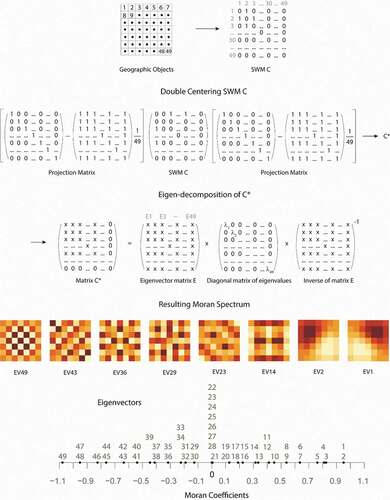
Corresponding to the 49 eigenvalues are 49 eigenvectors with descending MC values (from the right to the left); each can be visualized as a map, representing a distinct map pattern. Figure 2 depicts selected eigenvector maps and their MCs (in paratheses): $E{V}_1$ (0.95), $E{V}_2$ (0.95), $E{V}_{14}$ (0.32), $E{V}_{23}$ (0.0), $E{V}_{29}$ (−0.13), $E{V}_{36}$ (−0.32), $E{V}_{43}$ (−0.64), and $E{V}_{49}$ (−1.08). The SA patterns displayed by these maps are interpretable visually – when many similar values are clustered (e.g. $E{V}_1$), the map has a high positive MC value; when many dissimilar values are in local neighbours (e.g. $E{V}_{36}$), the map has a high negative MC value; when data values are haphazardly distributed (e.g. $E{V}_{23}$), the MC value is around 0. Several eigenvectors may have the same or similar MC values, appearing as stacked labels, revealing that different map patterns can have the same summary SA measurement. Most notably, $E{V}_1$ and $E{V}_2$ have the same MC but their map patterns are an orthogonal rotation of each other (Figure 2).

The metaphor of a light spectrum can be inserted here to enhance the explanation of the Moran Spectrum. A bean of sunlight, which has no apparent structure to the human eyes, turns into a rainbow of colours after passing through a prism. The prism decomposes the visible portion of solar radiation into spectral bands of different wavelengths. Mixing these rainbow colours produces the colourful world (in the human eyes). Similarly, a SWM, which appears as a collection of 1s and 0s, becomes a sequence of ‘component’ matrices through eigen-decomposition. This algebraic ‘prism’ produces the ‘rainbow’ of MC values in which each eigenvector represents a unique map pattern, facilitating in-depth analysis of geographic phenomena.

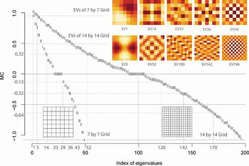
The Moran Spectrum reveals the characteristics of SA under different spatial configurations for the same area. For example, we can see what would happen if a geographic space is incrementally subdivided, such as the case in administrative and statistical regions, which results in more geographic units, and hence more rows and columns in the SWM. This creation of a finer geographic resolution renders a greater number of eigenvalues and eigenvectors across the domain of MC values. Figure 3 shows, when a 7-by-7 polygon grid is subdivided into a 14-by-14 polygon grid, the number of eigenvectors (and eigenvalues), or distinct map patterns, increase from $7^2=49$ to ${14}^2=196$, which leaves fewer gaps and registers more distinct map patterns having the same or similar MC values. For example, in the smaller 7-by-7 grid, there are 7 eigenvectors having a 0 MC; that number doubles to 15 in the 14-by-14 grid. The proportions of eigenvectors having MC values above or below 0 remain the same, about 0.5 (90 above 0 and 91 below 0, in the case of the 14-by-14 grid). The bounds of MC values, however, move closer to (−1, +1), from (−1.08, 0.95) to (−1.05, 1.02) as spatial resolution doubles in this situation. The increase of largest achievable positive MC is greater than the negative side. As Figure 3 depicts, for the 7-by-7 grid, eigenvalue #1 and its corresponding eigenvector EV1 register the maximum achievable positive MC for this geographic partitioning, at 0.95. For the 14-by-14 grid, the same MC value (0.95) corresponds to eigenvalue #5 and eigenvector EV5, four positions below the maximum MC of 1.02. The eigenvector maps, EV1 and EV5, appear differently. Except for the pair EV49 and EV196, the map patterns between the pairs EV14-EV52, EV23-EV100, and EV36-EV142, which have the same MC values, do not share much visual similarity. This comparison of Moran Spectrums at different spatial resolutions illustrates that an increase of spatial resolution leads to a greater level of positive SA, and visual analysis of SA patterns should be accompanied with statistics.

Figure 3. Comparisons of the Moran Spectrums for incremental spatial resolutions. The labels (EV1, EV14, EV23, EV36, EV49) and (EV5, EV52, EV100, EV142, EV196) are for EVs from the two different polygon grids.

Given a geographic variable, the Moran Spectrum can be used to show the specific eigenvectors associated with it. In this case, the eigenvectors in the Moran Spectrum are treated as potential covariates for a given geographic variable. Stepwise regression or other variable selection methods can then be used to identify which eigenvectors have a significant association with the geographic variable (Griffith and Chun 2021, 1891–1892). Figure 4 is a simulated geographic variable on a 7-by-7 polygon grid, which has a relatively high level of positive SA ($MC=0.72$). Out of the total 49 eigenvectors in the Moran Spectrum, 9 exhibit statistical significance through a forward-selection procedure. Ordered according to descending p-values, they are: EV1 (−15.69), EV4 (8.75), EV3 (−6.32), EV2 (−6.2), EV5 (−5.54), EV12 (5.52), EV6 (−3.5), EV7 (2.74), EV8 (1.8), with their regression coefficients (inside the paratheses) indicating their respective relative levels of importance. Figure 5 visualizes the map patterns of these eigenvectors and their positions on the Moran Spectrum. Figure 6 depicts their relative importance measured by the absolute values of their regression coefficients, a composite resembling spectral plots in remote sensing where the horizontal axis is the spectral bands and the vertical axis is the reflectance or emittance values for a given ground object.

Figure 4. Illustration of a specimen polygon data set.

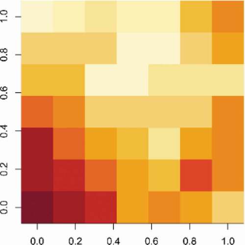
Figure 5. Significant eigenvectors accounting for SA in the geographic variable depicted in Figure 4. Top: eigenvector maps. Bottom: Moran Spectrum with the selected eigenvectors highlighted in bold.

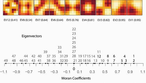
Figure 6. Regression coefficients, in absolute value, of significant eigenvectors associated with data in Figure 4. The background point plot depicts the positions of the selected eigenvectors in the Moran Spectrum (horizontal axis) constituting 49 eigenvectors.

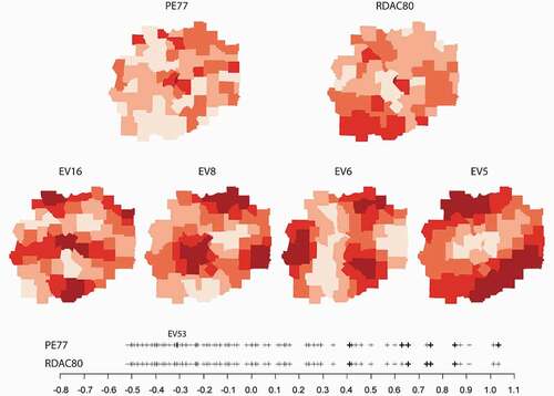
Similarly, for a pair of the geographic variables with the same spatial configuration (same SWM), their SA structures can be compared using the Moran Spectrum. Two variables from the St. Louis homicide data set,¹ PE77 (Police expenditures per capita, 1977) and RDAC80 (Resource deprivation/affluence composite variable, 1980), are used here for illustrative purpose (Figure 7). Both variables have significant positive SA, with $M{C}_{PE77}=0.19$ and $M{C}_{RDAC80}=0.3$. In order of p-values, PE77 is associated with EV1, EV16, EV8, EV5, EV6, EV9, and EV53, whereas RDAC80 has a significant relationship with EV8, EV5, EV7, and EV6. The two variables largely overlap in the positive region of the Moran Spectrum. PE77 however has a significant negative component EV53 ($MC=-0.31$), indicating a stronger spatial contrast in the distribution of PE77 where many high and low values are located next to each other. In this case, the decomposition of MC, a global measure, allows for a refined exploration of the SA that may lead to inclusion of negative SA components in model specifications (Hu, Chun, and Griffith 2020).

Figure 7. Common eigenvectors for the pair of attribute variables PE77 and RDAC80. Jenks method was used for map classification (five classes). Darker colours represent greater values.

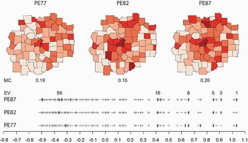
When there are multiple measurements of a given geographic variable over several time periods, the Moran Spectrum helps in assessing the spatio-temporal structure through a comparison of significant eigenvectors selected among the periods. For example, in the St. Loius homicide data set, PE (Police expenditures per capita) was available for three periods: 1977, 1982, and 1987. The significant eigenvectors associated with PE82 and PE87 were identified using forward selection, forming the temporal Moran Spectrum in Figure 8, revealing the time invariant EV5, EV8, and EV16, and an increasing number of eigenvectors associated with negative SA. The latter is an indication of increasing contrast with the spatial distribution of PE, which may lead to a series of research questions.

Figure 8. Significant eigenvectors associated with per capita Police Expenditure in the St. Louis area over three time periods. Eigenvectors selected for each period are symbolized as thicker bars. Those identified more than twice over the three periods are labelled with the eigenvector sequence numbers. Jenks method was used for map classification (five classes). Darker colours represent greater values.

We have so far shown how the Moran Spectrum helps in exploring SA. The most attractive application of the Moran Spectrum, however, is in statistical modelling of geographic variables, where a linear combination of selected eigenvectors from the Moran Spectrum forms a composite synthetic variable representing spatial structural information, i.e. for geographic variable column vector $y$,

(11) $y_i={\mu }_y+f\left(X_i\right)+f\left(S_i\right)+{\in }_i$(11)

(12) $S_i=E_{i1}{\gamma }_1+E_{i2}{\gamma }_2+\dots +E_{iK}{\gamma }_K=\sum _{K=1}^K{E}_{iK}{\gamma }_K$(12)

where $y_i$ is the ith observed attribute value, ${\mu }_y$ is the mean of variable $y$, $X$ is a row vector of covariates,${\in }_i$ is an iid (independently and identically distributed) random error term. $S_i$ is the ith value of the synthetic spatial variable generated by combining the products between the ith element of each eigenvector selected from the Moran Spectrum and the corresponding coefficient ${\gamma }_K$, with $K=1,2,\dots ,K$ being the number of eigenvectors selected. This linear combination of eigenvectors is referred to as an Eigenvector Spatial Filter (ESF), which is at the core of MESF theory and MEMs, serving as an alternative approach to representing SA in spatial modelling (Dray, Legendre, and Peres-Neto 2006; Griffith, Chun, and Bin 2019; Griffith 2010b; Legendre and Legendre 2012; Tiefelsdorf and Griffith 2007; Borcard and Legendre 2002).

Suppose we want to estimate the relationship between homicide rates and social economic conditions for the St. Louis homicide data set, with a bivariate linear regression model of the following form:

(13) $HR8893=a+b\left(RDAC90\right),$(13)

where HR8893 is homicide rates per 100,000 for the period 1988–1993 and RDAC90 is a resource deprivation/affluence composite variable, in 1990 (Messner et al. 1999). Both HR8893 and RDAC90 have significant positive SA ($M{C}_{HR8893}=0.2,M{C}_{RDAC90}=0.31$). The OLS estimation of the model in equation 11(11) $y_i={\mu }_y+f\left(X_i\right)+f\left(S_i\right)+{\in }_i$(11) results in $a=6.05\mathrm{a}\mathrm{n}\mathrm{d}b=4.71$; both are significant at $\alpha =0.05$, with a residual standard error of 5.19 and an adjusted R-squared ($R_{adj}^2$) of 0.26. The residual of this non-spatial model contains significant SA ($MC=0.37)$, indicating potential for improvement by incorporating SA information in the model. By using a spatial error model specification, $HR8893=a+b\left(RDAC90\right)+{\left(I-\lambda W\right)}^{-1}\in$, where $\lambda$ denotes a spatial autoregressive parameter and $W$ is the row-standardized SWM, residual SA is reduced to a non-significant trace amount of $MC=0.02$. 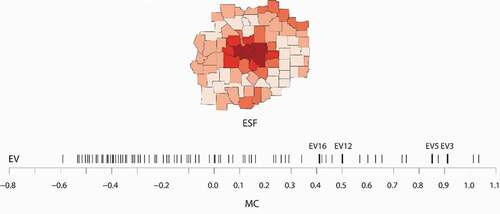In addition, the model fit increases to $R_{adj}^2=0.52$, and the residual standard error drops to 3.82. Alternatively, with the ESF approach, eigenvectors are selected to form a synthetic composite spatial variable from the Moran Spectrum through stepwise regression with the OLS residual as the dependent variable. Four eigenvectors are identified, in ascending order of p-values: EV5, EV3, EV16, and EV12. Including them as covariates forms the following expanded OLS model:

(14) $HR8893=a+b\left(RDAC90\right)+\left({\gamma }_{1}E{V}_5+{\gamma }_{2}E{V}_3+{\gamma }_{4}E{V}_{16}+{\gamma }_{5}E{V}_{12}\right)$(14)

These eigenvectors serve as surrogates for omitted spatial variables in the conventional non-spatial model (i.e. Equation 13)(13) $HR8893=a+b\left(RDAC90\right),$(13) . Figure 9 depicts the positions of these eigenvectors in the Moran Spectrum and the map pattern of their linear combination, the ESF, which captures positive SA ($MC=0.7$). The ESF filters the SA from the OLS residual and moves the SA information to the intercept, correcting the misspecification of the original OLS model. Consequently, residual SA is largely filtered out, with $MC=0.005$ and not significant. The residual standard error drops to 3.16. and the model fit increases to $R_{adj}^2=0.62$. Using the non-spatial OLS as the baseline model, the ESF-OLS model shows 35% of the variation in HR8893 is due to SA. The ESF-OLS also produced a better fit than the spatial error model.

Figure 9. A sum of selected eigenvectors weighted by their respective regression coefficients form the synthetic composite spatial variable ESF = (−12.9804) EV3 + (−27.3753) EV5 + (9.3323) EV12 + (10.6957) EV16.

Treating SA embedded in a geographic variable as a mixture of eigenvector components in the Moran Spectrum opens a new horizon in spatial statistical modelling. The fundamental breakthrough comes from the quantitative generalization of SA structure embedded in geographic processes as a synthetic variable; i.e. a linear combination of relevant eigenvectors, effectively representing the spatial component for any geographic variable. By adding this synthetic variable to its affiliated statistical model, SA information left in the residual is filtered out and added back into a model’s intercept term (i.e. a constant intercept becomes a variable intercept), resulting in a substantial improvement in statistical inference and prediction.

Acting like an additional covariate in regression models, ESF has the advantage of accounting for SA without altering the likelihood functions or regression equation description forms of geographic variables, and hence reducing methodological as well as computational complexities, particularly in the cases of non-Gaussian variables such as a binomial and Poisson (Besag 1972; Griffith, 2002, 2004, 2010; Kaiser & Cressie 1997). Because an ESF can capture local as well as regional and global SA structures, different levels of associations between the geographic variable and the covariates can be estimated by adding selected interaction terms between chosen eigenvectors from the Moran Spectrum and the covariates, providing an alternative to Geographically Weighted Regression (GWR) (Fotheringham, Brunsdon, and Charlton 2002; Gelfand et al. 2003; Griffith 2008; Griffith, Chun, and Bin 2019; Waller et al. 2007), effectively addressing the issue of spatial heterogeneity. The MESF approach can be directly extended to space-time modelling by representing spatial and temporal autocorrelation with a space-time weights matrix (STWM). Eigen-decomposition of the doubly centre STWM produces the space-time Moran Spectrum, anchored by the space-time eigenvalues and eigenvectors. For a given space-time geographic variable data set, a Moran Eigenvector Space-Time Filter (MESTF) can be formulated, accounting for both spatial and temporal autocorrelation (Griffith 2012; Griffith, Chun, and Bin 2019). Finally, in modelling spatial interactions, the MESF approach makes accounting for SA in both origin and destination model components straight-forward (Chun & Griffith 2011; Griffith 2009; Griffith & Chun 2015). As software tools have become available (Bivand et al. 2013; Murakami 2017; Koo, Chun, and Griffith 2018), applications of MESF and MEMs have steadily increased across the social science as well as environmental and health science disciplines (Fischer & Getis 2009; Griffith & Chun 2021; Griffith et al. 1999; Tan et al. 2020; Zhang et al. 2018).

Discussion

The Moran Spectrum represents the FLG as a combination of diagrammatic, graphic, and numerical representations. It is a practice of the Tupu methodology and a realization of a major goal of Geoinformatic Tupu to represent the general principles of geographic processes in five fundamental ways. First, it is based upon the recognized geographic principle known as the FLG. The MC, along with the specification of spatial relationships by a SWM, provides for a mathematical formularization of the FLG. And the algebraic principle of eigen-decomposition is the ultimate tool enabling the formation of the Moran Spectrum. Second, it is a top-down decomposition of a complex system; in this case, the spatial structure of a given geographic landscape. Although a sequence of thematic maps can show the physical appearance of a geographic variable, MEMs reveal persistent SA structure underlying a data generating process, and the corresponding eigenvalues index the range and intervals of prevailing distinct MCs. These intervals shorten as spatial resolution increases, analogous to the increasing spectral resolution in remote sensing. Third, the Moran Spectrum is an ordered system of distinct SA patterns with sequential values of MCs. Any observed SA pattern is a function of the combination of a subset of these reference patterns (eigenvectors) and values (eigenvalues) (Boots and Tiefelsdorf 2000). Fourth, the eigen-decomposition results in a binary system – positive and negative SA corresponding to a split in the sequence of eigenvalues and their corresponding MEMs (Griffith and Luhanga 2011). Although most spatial processes are dominated by positive SA, the observed MC can contain components of negative SA, which are buried in an MC index but can be extracted from the Moran Spectrum. Separating the mixture of SA and uncovering negative SA allow more detailed spatial analysis. Last but not least, the Moran Spectrum is both visual and functional. The eigenvector maps show the sequence of distinct patterns of SA. The plot of eigenvectors associated with a given geographic variable shows the contributing structural components. The synthetic variable formed by a linear combination of selected eigenvectors serves as the surrogate of spatial structural information, accounting for geographic effects on variable variation, leading to a substantial improvement of model performance in statistical prediction and inferences. Therefore, the Moran Spectrum is a systematic generalization of the FLG and a genuine Tupu. Because spatial relationships are fundamental in geospatial analysis, and FLG is universal in geospatial processes, the Moran Spectrum should be considered an essential component in Geoinformatic Tupu.

Meanwhile, structural characteristics for geographic phenomena are multifaceted. SA is one of them; SWM is one way to represent the FLG; and MC is one of many approaches to quantifying SA. Hence a Moran Spectrum represents only one – although a very important one – aspect of spatial structure. Other approaches, notably the semivariogram-based conceptualization of SA, for example, also can be generalized in the Tupu context. Other types of spatial structural characteristics, such as rank-size rules (e.g. power laws) and rhythmic patterns, need different representations.

Furthermore, structural characteristics of geospatial phenomena are multi-scale and multi-dimensional. We illustrated the possibility of constructing Moran Spectra at multiple scales and referenced the possibility of extending this notion to space-time dimensions. The constraint for forming the multi-scale Moran Spectra for polygon features is that the system of hierarchical partitioning needs to be nested. Administrative regions mostly satisfy this requirement, while functional regions may not be nested between scales. This limitation can be alleviated if spatial features can be represented as points; in such cases, distance-based SWMs have the multi-scale flexibility (Legendre and Legendre 2012; Murakami 2017). For space-time systems, the Moran Spectrum is a mathematical extension of the two-dimensional approach, assuming a SA structure does not change over time. Such an assumption may be challenged when the original landscape is transformed due to infrastructure development or environmental changes. New methods need to be developed for dynamic spatial and temporal structures. Such an extension also needs to be made in the three-dimensional space where many geospatial processes take place.

Conclusion

The Moran Spectrum as a Geoinformatic Tupu provides a representation of the FLG. A new set of Exploratory Spatial Data Analysis (ESDA) tools can be developed for exploring spatial dependence structures for individual variables, multiple variables, and in both spatial and temporal dimensions. MESF-based regression modelling also can be presented in this Tupu framework, making it more accessible conceptually and interpretable in practice. In a broader context, the Moran Spectrum has the potential to serve as a reference system of relative distance, where the relationship between geographic objects is measured by spatial autocorrelation instead of physical distance, similar to genetic maps where the recombination frequencies are the distances between genes.

Presenting the Moran Spectrum in the context of Geoinformatic Tupu turned out to be a productive process in explaining its methodology and applications, and in refining our understanding of Geoinformatic Tupu. We presented a convincing case that the Moran Spectrum is a Geoinformatic Tupu, and should be an inherent component of a Geoinformatic Tupu because SA is embedded in all geographic processes. Incorporating SA in spatial analysis can be as straight-forward as selecting components from the Moran Spectrum, a Geoinformatic Tupu. Using an ESF constructed from a Moran Spectrum to represent spatial structure information in spatial modelling opens a promising new path to spatial modelling, which presents opportunities for research and development. On the theoretical front, the effects of SWM specification is a core issue. As there are many ways a SWM can be specified for the same georeferenced variable, the effects of different specifications on the construction of an ESF and the resulting spatial model need to be further investigated through sensitivity analysis. Another issue with MESF-based spatial modelling is overfitting where out-of-sample prediction error is much greater than training error (James et al. 2013), as inclusion of a large number of eigenvectors as covariates in estimating a regression model may result in fitting some random variation and artificially inflating goodness-of-fit statistics. Overfitting is particularly challenging for MESF-based heterogeneity analysis, which requires interaction terms between the covariates and the eigenvectors (Oshan and Fotheringham 2018), often resulting in a candidate set whose size is much larger than n. Cross-validation selection techniques offer one way to address this complication.

A broad adoption of Moran Spectrum-based analysis also faces some computational challenges. Eigen-decomposition of a SWM, the core operation, has a complexity of $O\left(n^3\right)$, and hence presents a computational problem for large datasets. Although eigenvalues and eigenvectors can be approximated for regular square tessellations, no such estimates are available for SWMs of irregular tessellations (Griffith 2015). Because spatial partitions of a region often have a long duration, a bank of Moran Spectra can be generated and made available for online access, similar to gene maps in molecular biology. Selection of eigenvectors from a reference set of eigenvectors to form an ESF is a more challenging problem. Traditional methods of automatic selection represented by forward selection, backward elimination, and stepwise regression are computationally intensive and not practical for large datasets, particularly for raster data and generalized linear modelling regression. Different approaches have been proposed to deal with large datasets (Seya et al. 2015; Murakami and Griffith 2017; Yang et al. 2018; Griffith, Chun, and Bin 2019), where are in need of further testing and improvement for real-world applications.

Finally, three realizations about the current definition of Geoinformatic Tupu are noteworthy. First, visual processing, considered as a core component in the current definition of Geoinformatic Tupu, should be used along with quantitative analysis. We show in this paper that two eigenvector maps with different visual patterns can have the same MC values. Second, the computational aspects of Geoinformatic Tupu should be emphasized, which should go beyond traditional digital cartographic operations. The Moran Spectrum is computational in that it generates a synthetic composite variable that can be used in virtually all spatial modelling. Finally, the time dimension, currently considered an essential component in Geoinformatic Tupu, does not have to be explicitly present. Moran Spectra can be viewed as results of temporal processing while not being temporal time series themselves. This observation does not contradict empirical examples of Geo-Tupu for which an Earth tectonic map and a map of climate zones are considered to be Tupu. These realizations, together with the proposed inclusion of the Moran Spectrum as an explicit representation of spatial relationships in Geoinformatic Tupu, furnish considerable opportunity to contribute to the theoretical as well as technical development of Geographic Information Sciences in general, and Geoinformatic Tupu in particular.

Disclosure statement

No potential conflict of interest was reported by the author(s).

Notes

1. The data set is made available by the GeoDA Center at https://geodacenter.github.io/data-and-lab/stlouis/

References

- Anselin, L. 1984. “.” In Papers of the Regional Science Association. Vol. 54, 165–182. .
- Anselin, L. 1988. Spatial Econometrics: Methods and Models. Dordrecht, The Netherlands: Kluwer Academic Publishers.
- Besag, Julian E. 1972. “Nearest-Neighbour Systems and the Auto-Logistic Model for Binary Data.” Journal of the Royal Statistical Society. Series B (Methodological), 75–83.
- Bivand, R. S., E. J. Pebesma, and V. Gomez-Rubio. 2013. Applied Spatial Data Analysis with R. 2nd ed. New York: Springer.
- Boots, B., and M. Tiefelsdorf. 2000. “Global and Local Spatial Autocorrelation in Bounded Regular Tessellations.” Journal of Geographical Systems 2 (4): 319–348. doi:https://doi.org/10.1007/PL00011461.
- Borcard, D., and P. Legendre. 2002. “All-Scale Spatial Analysis of Ecological Data by Means of Principal Coordinates of Neighbour Matrices.” Ecological Modelling 153 (1–2): 51–68. doi:https://doi.org/10.1016/S0304-3800(01)00501-4.
- Chen, S. 1998. “Dìxué Xìnxī Túpǔ Chúyì [Discussion on Geoinformation Tupu].” Dìlǐ Yánjiū [Geographical Research] 17 (Supplement): 5–9.
- Chen, S. 1999. Chénshù Péng Yuànshì Kēxué Xiǎopǐn Xuǎnjí [Selection of Chen Shupeng’s Science Essays]. Beijing: China Environmental Press.
- Chen, S. 2001. Dìxué Xìnxī Túpǔ Tànsuǒ Yánjiū [Exploring Research on Geoinformatic Tupu]. Beijing: Commercial Press.
- Chun, Y., and D. A. Griffith. 2013. Spatial Statistics and Geostatistics: Theory and Applications for Geographic Information Science and Technology. Los Angeles: SAGE Publications.
- Chun, Yongwan, and Daniel A. Griffith. 2011. “Modeling Network Autocorrelation in Space–Time Migration Flow Data: An Eigenvector Spatial Filtering Approach.” Annals of the Association of American Geographers 101 (3): 523–36.
- Cliff, A. D., and J. K. Ord. 1973. Spatial Autocorrelation. Vol. 5. London: Pion.
- Cliff, A. D., and J. K. Ord. 1981. Spatial Processes: Models & Applications. Vol. 44. London: Pion.
- Cressie, N. 1993. Statistics for Spatial Data. New York: John Wiley & Sons.
- de Jong, P., C. Sprenger, and F. Van Veen. 1984. “On Extreme Values of Moran’s I and Geary’s C.” Geographical Analysis 16 (1): 17–24. doi:https://doi.org/10.1111/j.1538-4632.1984.tb00797.x.
- Dray, S., P. Legendre, and P. R. Peres-Neto. 2006. “Spatial Modelling: A Comprehensive Framework for Principal Coordinate Analysis of Neighbour Matrices (PCNM).” Ecological Modelling 196 (3–4): 483–493. doi:https://doi.org/10.1016/j.ecolmodel.2006.02.015.
- Fotheringham, A. S., C. Brunsdon, and M. Charlton. 2002. Geographically Weighted Regression: The Analysis of Spatially Varying Relationships. 1st ed. Chichester, UK: John Wiley & Sons.
- Gelfand, A. E., H.-J. Kim, C. F. Sirmans, and S. Banerjee. 2003. “Spatial Modeling with Spatially Varying Coefficient Processes.” Journal of the American Statistical Association 98 (462): 387–396. doi:https://doi.org/10.1198/016214503000170.
- Getis, A. 2009. “Spatial Weights Matrices.” Geographical Analysis 41 (4): 404–410. doi:https://doi.org/10.1111/j.1538-4632.2009.00768.x.
- Getis, A. 2010. “Spatial Autocorrelation.” In Handbook of Applied Spatial Statistics, 255–278. New York: Springer.
- Goodchild, M.F. 2009. “First Law of Geography.” In International Encyclopedia of Human Geography, 179–182. Amsterdam, The Netherlands: Elsevier.
- Griffith, D., and B. Li. 2017. “A Geocomputation and Geovisualization Comparison of Moran and Geary Eigenvector Spatial Filtering.” 25th International Conference on Geoinformatics, August 2-4, 2017, Buffalo, NY, 1–4. IEEE.
- Griffith, D., and U. Luhanga. 2011. “Approximating the Inertia of the Adjacency Matrix of a Connected Planar Graph that Is the Dual of a Geographic Surface Partitioning.” Geographical Analysis 43 (4): 383–402. doi:https://doi.org/10.1111/j.1538-4632.2011.00828.x.
- Griffith, D., and Y. Chun. 2021. “Spatial Autocorrelation and Spatial Filtering.” In Handbook of Regional Science, 2nd ed., 1891–92. Berlin: Springer-Verlag.
- Griffith, D., Y. Chun, and B Li. 2019. Spatial Regression Analysis Using Eigenvector Spatial Filtering. San Diego, CA: Academic Press.
- Griffith, D. 1996. “Spatial Autocorrelation and Eigenfunctions of the Geographic Weights Matrix Accompanying Geo-Referenced Data.” Canadian Geographer/Le Géographe Canadien 40 (4): 351–367. doi:https://doi.org/10.1111/j.1541-0064.1996.tb00462.x.
- Griffith, D. 2003. Spatial Autocorrelation and Spatial Filtering: Gaining Understanding through Theory and Scientific Visualization. New York: Springer.
- Griffith, D. 2008. “Spatial-Filtering-Based Contributions to a Critique of Geographically Weighted Regression (GWR).” Environment & Planning A 40 (11): 2751–2769. doi:https://doi.org/10.1068/a38218.
- Griffith, D. 2010a. “The Moran Coefficient for Non-Normal Data.” Journal of Statistical Planning and Inference 140 (11): 2980–2990. doi:https://doi.org/10.1016/j.jspi.2010.03.045.
- Griffith, D. 2010b. Spatial Autocorrelation and Spatial Filtering: Gaining Understanding through Theory and Scientific Visualization. Softcover reprint of hardcover 1st ed. Softcover reprint of hardcover ed. New York: Springer.
- Griffith, D. 2012. “Space, Time, and Space-Time Eigenvector Filter Specifications that Account for Autocorrelation.” Estadística Española 54 (177): 7–34.
- Griffith, D. 2015. “Approximation of Gaussian Spatial Autoregressive Models for Massive Regular Square Tessellation Data.” International Journal of Geographical Information Science 29 (12): 1–31.
- Griffith, D. 2019. “Negative Spatial Autocorrelation: One of the Most Neglected Concepts in Spatial Statistics.” Stats 2 (3): 388–415. doi:https://doi.org/10.3390/stats2030027.
- Griffith, Daniel A. 2002. “A Spatial Filtering Specification for the Auto-Poisson Model.” Statistics & Probability Letters 58 (3): 245–51.
- Griffith, Daniel A. 2004. “A Spatial Filtering Specification for the Autologistic Model.” Environment and Planning A 36 (10): 1791–1811.
- Griffith, Daniel A. 2009. “Spatial Autocorrelation in Spatial Interaction.” In Complexity and Spatial Networks, 221–37. Springer.
- Griffith, Daniel A. 2010. “The Moran Coefficient for Non-Normal Data.” Journal of Statistical Planning and Inference 140 (11): 2980–90. https://doi.org/https://doi.org/10.1016/j.jspi.2010.03.045.
- Griffith, Daniel A., Larry J. Layne, John Keith Ord, and Akio Sone. 1999. A Casebook for Spatial Statistical Data Analysis: A Compilation of Analyses of Different Thematic Data Sets. Oxford University Press on Demand.
- Griffith, Daniel A., and Yongwan Chun. 2015. “Spatial Autocorrelation in Spatial Interactions Models: Geographic Scale and Resolution Implications for Network Resilience and Vulnerability.” Networks and Spatial Economics 15 (2): 337–65.
- Griffith, D. 2017. “Spatial Weights.“ In International Encyclopedia of Geography, edited by Kobayashi, Audrey, Richardson, D., Goodchild, M., Castree, N., Marston, R., and Liu, W.eds., 1–14. Chichester, UK: John Wiley & Sons.
- Hu, L., Y. Chun, and D. A. Griffith. 2020. “Uncovering a Positive and Negative Spatial Autocorrelation Mixture Pattern: A Spatial Analysis of Breast Cancer Incidences in Broward County, Florida, 2000–2010.” Journal of Geographical Systems 22 (3): 291–308. doi:https://doi.org/10.1007/s10109-020-00323-5.
- Huangyuan Tan, Yumin Chen, John P. Wilson, Jingyi Zhang, Jiping Cao, and Tianyou Chu. 2020. “An Eigenvector Spatial Filtering Based Spatially Varying Coefficient Model for PM2. 5 Concentration Estimation: A Case Study in Yangtze River Delta Region of China.” Atmospheric Environment 223: 117205.
- James, G., D. Witten, T. Hastie, and R. Tibshirani. 2013. An Introduction to Statistical Learning: With Applications in R. New York: Springer Science & Business Media. http://www-bcf.usc.edu/~gareth/ISL/index.html.
- Kaiser, Mark S., and Noel Cressie. 1997. “Modeling Poisson Variables with Positive Spatial Dependence.” Statistics & Probability Letters 35 (4): 423–32.
- Koo, H., Y. Chun, and D. A. Griffith. 2018. “Integrating Spatial Data Analysis Functionalities in a GIS Environment: Spatial Analysis Using ArcGIS Engine and R (SAAR).” Transactions in GIS 22 (3): 721–736. doi:https://doi.org/10.1111/tgis.12452.
- Legendre, P., and L. Legendre. 2012. Numerical Ecology. Amsterdam, The Netherlands: Elsevier.
- Li, B. 1995. “Implementing Spatial Statistics on Parallel Computers.” In Practical Handbook of Spatial Statistics, 107–148. Boca Raton, FL: CRC Press.
- Liao, K. 2001. “Zhōngguó Zìrán Jǐngguān Zònghé Xìnxī Túpǔ de Jiànlì Yuánzé Yǔ Fāngfǎ [Principles and Methods of Designing and Establishing Complex Informatic Tupu of Natural Landscape in China].” Acta Geographica Sinica 56 (B09): 19–25.
- Luo, Q., D. A. Griffith, and H. Wu. 2019. “Spatial Autocorrelation for Massive Spatial Data: Verification of Efficiency and Statistical Power Asymptotics.” Journal of Geographical Systems 21 (2): 237–269. doi:https://doi.org/10.1007/s10109-019-00293-3.
- Messner, S., L. Anselin, R. Baller, D. Hawkins, G. Deane, and S. Tolnay. 1999. “The Spatial Patterning of County Homicide Rates: An Application of Exploratory Spatial Data Analysis.“ Journal of Quantitative Criminology 15 (4): 423–450.
- Moran, P. A. P. 1950. “Notes on Continuous Stochastic Phenomena.” Biometrika 37 (1/2): 17–23. doi:https://doi.org/10.1093/biomet/37.1-2.17.
- Murakami, D. 2017. “Spmoran: An R Package for Moran’s Eigenvector-Based Spatial Regression Analysis.” ArXiv Preprint ArXiv:1703.04467.
- Murakami, D., and D. A. Griffith. 2017. “Eigenvector Spatial Filtering for Large Data Sets: Fixed and Random Effects Approaches.” Geographical Analysis 51 (1): 23–49.
- Oshan, T. M., and A. S. Fotheringham. 2018. “A Comparison of Spatially Varying Regression Coefficient Estimates Using Geographically Weighted and Spatial-Filter-Based Techniques.” Geographical Analysis 50 (1): 53–75. doi:https://doi.org/10.1111/gean.12133.
- Qi, Q., and T. Chi. 2001. “Dìxué Xìnxī Túpǔ de Lǐlùn Hé Fāngfǎ [Theories and Methods of Geoinformatic Tupu].” Acta Geographica Sinica 56 (7s): 8–18.
- Qi, Q. 2004. “Dìxué Xìnxī Túpǔ de Zuìxīn Jìnzhǎn [The Latest Development of Geoinformatic Tupu].” Cèhuì Kēxué [Science of Survey and Mapping] 29 (6): 15–23.
- Seya, H., D. Murakami, M. Tsutsumi, and Y. Yamagata. 2015. “Application of LASSO to the Eigenvector Selection Problem in Eigenvector-Based Spatial Filtering.” Geographical Analysis 47 (3): 284–299. doi:https://doi.org/10.1111/gean.12054.
- Strang, G. 2016. Introduction to Linear Algebra. 5th ed. Wellesley, MA: Wellesley-Cambridge Press.
- Tiefelsdorf, M., and B. Boots. 1995. “The Exact Distribution of Moran’s I.” Environment & Planning A 27 (6): 985. doi:https://doi.org/10.1068/a270985.
- Tiefelsdorf, M., and D. A. Griffith. 2007. “Semiparametric Filtering of Spatial Autocorrelation: The Eigenvector Approach.” Environment & Planning A 39 (5): 1193. doi:https://doi.org/10.1068/a37378.
- Tobler, W. R. 1970. “A Computer Movie Simulating Urban Growth in the Detroit Region.” Economic Geography 46: 234–240. doi:https://doi.org/10.2307/143141.
- Waller, L. A., L. Zhu, C. A. Gotway, D. M. Gorman, and P. J. Gruenewald. 2007. “Quantifying Geographic Variations in Associations between Alcohol Distribution and Violence: A Comparison of Geographically Weighted Regression and Spatially Varying Coefficient Models.” Stochastic Environmental Research and Risk Assessment 21 (5): 573–588. doi:https://doi.org/10.1007/s00477-007-0139-9.
- Xu, J., T. Pei, and Y. Yao. 2010. “Dìxué Zhīshì Túpǔ de Dìngyì, Nèihán Hé Biǎodá Fāngshì de Tàntǎo [Conceptual Framework and Representation of Geographic Knowledge Map].” Journal of Geo-Information Science 12 (4): 496–502. doi:https://doi.org/10.3724/SP.J.1047.2010.00496.
- Yang, J., Y. Chen, M. Chen, F. Yang, and M. Yao. 2018. “A Segmented Processing Approach of Eigenvector Spatial Filtering Regression for Normalized Difference Vegetation Index in Central China.” ISPRS International Journal of Geo-Information 7 (8): 330. doi:https://doi.org/10.3390/ijgi7080330.
- Zhang, H., C. Zhou, L. Guonian, Z. Wu, F. Lu, J. Wang, T. Yue, J. Luo, Y. Ge, and C. Qin. 2020. “Shì Lùn Dìxué Xìnxī Túpǔ Sīxiǎng de Nèihán Yǔ Chuánchéng [The Connotation and Inheritance of Geoinformation Tupu].” Journal of Geo-Information Science 22 (4): 653–661. doi:https://doi.org/10.12082/dqxxkx.2020.200167.
- Zhang, Jingyi, Bin Li, Yumin Chen, Meijie Chen, Tao Fang, and Yongfeng Liu. 2018. “Eigenvector Spatial Filtering Regression Modeling of Ground PM2. 5 Concentrations Using Remotely Sensed Data.” International Journal of Environmental Research and Public Health 15 (6): 1228.
- Zhang, R. 2009. “Dìxué Xìnxī Túpǔ Yánjiū Jìnzhǎn [Research Progress of Geoinformatic Tupu].” Cèhuì Kēxué [Science of Survey and Mapping] 34 (1): 14–16.
- Zhou, C., and B. Li. 1998. “Dìqiú Kōngjiān Xìnxī Túpǔ Chūbù Tàntǎo [Preliminary Discussion on Geoinformatic Tupu].” Dìlǐ Yánjiū [Geographical Research] 17 (S1): 10–16.
- Zhou, C., X. Zhu, M. Wang, C. Shi, and Y. Ou. 2011. “Quánxí Wèizhì Dìtú Yánjiū [Research on Holographic Location Map].” Dìlǐ Kēxué Jìnzhǎn [Progress in Geographical Science] 30 (11): 1331–1335.