Integrating fuzzy set function into floating catchment area measures: a determination of spatial accessibility of service points

ABSTRACT

The use of discrete (binary or zonal/step-wise) instead of continuous travel impedance functions in floating catchment area (FCA) measures generates inconsistent and less reliable accessibility indices that might be overestimating or underestimating actual accessibility. Thus, this study illustrates the limitations of discrete travel impedance function in the enhanced two-step (E2S) FCA method; and develops a fuzzy-based continuous travel impedance function by combining the degree to which travel distances belong to different sub-zones of catchment areas and their respective E2SFCA zonal weights using the weighted mean fuzzy-set operation. With the developed fuzzy-based travel impedance function, a new accessibility measure, fuzzy-based two-step (F2S) FCA is defined. The E2SFCA and F2SFCA measures were implemented in the hypothetical set up and Rural Wards of Dodoma Urban District in Tanzania to determine spatial accessibility of service points and water points, respectively. The resulting E2SFCA and F2SFCA accessibility indices portrayed a slightly similar pattern. However, F2SFCA accessibility indices varied among households within and across sub-zones, while E2SFCA accessibility indices were identical within but changed abruptly across sub-zones. The variations in F2SFCA accessibility indices reflect the reality and to a greater extent Tobler’s first law of Geography. Thus, the developed F2SFCA measure could be used to measure spatial accessibility of other services or commodities as it properly models travel impedance. The F2SFCA measure could further be improved to generate much more realistic accessibility indices by capturing local instead of total potential demand, commonly modelled in FCA measures.

KEYWORDS:

• Households
• Floating Catchment Area (FCA)
• fuzzy-based travel impedance function
• Geographic Information System (GIS)
• spatial accessibility of water points

1. Introduction

In the 1950s, Hansen conceived accessibility as the potential of opportunities for interaction based on Stewart’s concept of population potential (Hansen 1959). This conception of accessibility is concerned with measuring the spatial distribution of activities about a point, adjusted by the ability and desire of the population to overcome spatial separation (Hansen 1959). However, the spatial distribution of potential opportunities (i.e. service points) and population (i.e. service users) within a region is usually uneven, making the population’s spatial access to services inequitable (Luo 2014). Thus, more accurate and reliable analysis of potential spatial accessibility of services (or amenities) is critical for effective service planning and allocation. The analyses of spatial accessibility are based on the location and capacity of service points, location and demand of service users and travel distance between service users and service points (Bauer et al. 2020; Chen 2019; Delamater 2013; Joseph and Bantock 1982; Luo 2014; Ni et al. 2019).

Several measures have been developed and applied to measure the potential spatial accessibility of services. The modified gravity-based measure proposed by Joseph and Bantock (1982) is more sophisticated than proximity-based or cumulative-based measures as it considers potential service capacity, potential population demand for services and physical accessibility (Joseph and Bantock 1982; Schuurman, Bérubé, and Crooks 2010). With the modified gravity-based measure, both the potential capacity and demand are modified by the travel distance. Thus, the gravity-based measures address the shortcomings of generating homogeneous accessibility indices and not counting the cross-border interaction in the coverage-based measures (Bryant and Delamater 2019; Chen 2019; Zhu et al. 2019). However, the gravity-based measures require a pre-defined appropriate distance decay function with the appropriate impedance coefficient, which represents the change in the difficulty of travelling as travel distance changes (Guagliardo 2004). A distance decay function is usually unknown, varies with social context, takes many mathematical forms (i.e. linear or exponential) and is established using regression analysis and actual service utilization data (Guagliardo 2004; Schuurman, Bérubé, and Crooks 2010). Though service utilization data could be obtained through field surveys, they are often unavailable and become the main drawback of gravity-based measures (Schuurman, Bérubé, and Crooks 2010). Due to this drawback of gravity-based measures, impedance functions of different coefficients have been defined by different scholars based on published precedents (Joseph and Bantock 1982; Luo 2014; Mahuve, Liwa, and Chaula 2015) or their assumption (Bryant and Delamater 2019; Chen 2019; Schuurman, Bérubé, and Crooks 2010; Zhu et al. 2019).

The two-step floating catchment area (2SFCA) measure developed by Radke and Mu (2000) and pioneered by Luo and Wang (2003) has been proven to be a special case of the gravity-based accessibility measure, which, instead of continuous, uses dichotomous impedance function (Wu et al. 2018; Zhou et al. 2021). Though the 2SFCA measure considers the interaction between service providers and users across borders and generates accessibility indices varying from one area to another, it draws an artificial line at the threshold distance (say 400 m) between accessible and inaccessible services (Cheng et al. 2020; Shaw and Sahoo 2020; Wang and Luo 2005). As a result, services are considered to be equally delivered to population units within the threshold distance and fully accessed by each population unit regardless of the travel distance (Cheng et al. 2020; Liu et al. 2020; McGrail 2012; Wu et al. 2018; Zhou et al. 2021). Over the last two decades, the 2SFCA method has undergone several improvements that aimed at overcoming its limitations linked with the use of uniform catchment size (W. Luo and Whippo 2012; Su, Chen, and Cheng 2021; Tao et al. 2020), omission of distance decay function (J. Bauer et al. 2020; Bauer, Groneberg, and Deribe 2016; Dai and Wang 2011; Freeman et al. 2020; W. Luo and Qi 2009; Subal, Paal, and Krisp 2021; Zheng et al. 2020), travel behaviour (i.e. modes of travel) (Hu et al. 2020; Lin et al. 2018; Tao et al. 2018) and demand and supply modelling (Bozorgi et al. 2021; Delamater 2013; Kim et al. 2021; J. Luo 2016; Paez et al. 2019; Wan, Zou, and Sternberg 2012). Recently, the step-wise, also called the enhanced (E) (Ghorbanzadeh et al. 2021; Kar et al. 2021; Kiani et al. 2021; Mohammadi et al. 2021; Peng 2020; T. Xia et al. 2019; Zahnd et al. 2021) and Gaussian-based (G) (Bryant and Delamater 2019; Chen 2019; Li et al. 2021; Stewart et al. 2020; Xiao, Wei, and Wan 2021; Zhu et al. 2019), 2SFCA have been the most dominant 2SFCA methods addressing the limitations due to omission of distance decay function. The G2SFCA method is slightly different from the modified gravity-based method as it considers all demand and services within fixed or variable catchment sizes, while the modified gravity-based method considers all demand and services within the area of interest (i.e. the study area). Though both the modified gravity-based method and the G2SFCA method use a continuous distance decay function, they suffer from the difficulties of defining the travel impedance coefficient, which requires modelling of the actual service utilization. On the contrary, the E2SFCA method uses pre-defined discrete/zonal weights, which are uniform within each zone and thus less realistic. Since the number of zones defined in the E2SFCA method are considerably few, two to four zones, it is practicable to weigh zones by comparing their influence on accessibility. However, a single weight assigned to each zone hides the varying influence of different travel distances within each zone. Thus, this study aims at assigning different weights to different travel distances within each zone based on the E2SFCA pre-defined zonal weights.

1.1. The enhanced two-step floating catchment area measure

Luo and Qi (2009) enhanced the 2SFCA measure and partially addressed its shortcoming of generating homogenous accessibility indices within the threshold distance that defines a catchment area (Dai and Wang 2011). They incorporated the travel impedance function into the 2SFCA method to account for differential travel distance within catchment areas. In the first step, the E2SFCA method divides the catchment of each service site into several sub-zones ($D_r$), assigns travel impedance weights ($W_r$) to each sub-zone based on travel impedance function [$f\left(d_{ij}\right)$], calculates the potential demand ($D_j$) for each service site modified by the travel impedance weight and finally, using Equation (1)(1) $R_j=\frac{S_j}{D_j}=\frac{S_j}{{\sum }_{k\in \left\{d_{kj}\in D_r\right\}}{P}_k{W}_r}=\frac{S_j}{{\sum }_{k\in \left\{d_{kj}\in D_1\right\}}{P}_k{W}_1+{\sum }_{k\in \left\{d_{kj}\in D_2\right\}}{P}_k{W}_2+.\hspace{0.17em}.\hspace{0.17em}.}$(1) calculates the supply-to-demand ratio (i.e. the level of service) ($R_j$) for each service site (Luo and Qi 2009).

(1) $R_j=\frac{S_j}{D_j}=\frac{S_j}{{\sum }_{k\in \left\{d_{kj}\in D_r\right\}}{P}_k{W}_r}=\frac{S_j}{{\sum }_{k\in \left\{d_{kj}\in D_1\right\}}{P}_k{W}_1+{\sum }_{k\in \left\{d_{kj}\in D_2\right\}}{P}_k{W}_2+.\hspace{0.17em}.\hspace{0.17em}.}$(1)

where $S_j$ is the size of supply at location $j$, $D_j$ is the potential demand for supply $j$, $P_k$ is the population at site $k$ falling within the catchment (i.e. $d_{kj}\in D_r$), $d_{kj}$ is the travel impedance between supply $j$ and population $k$, $D_r$ is the travel impedance zone (i.e. subzone) and $W_r$ is the travel impedance weight for $D_r$.

In the second step, the E2SFCA method divides the catchment of each population site into several sub-zones ($D_r$), assigns travel impedance weights ($W_r$) to each sub-zone based on travel impedance function [$f\left(d_{ij}\right)$] and applies Equation (2)(2) $A_i=\sum _{j\in \left\{d_{ij}\in D_r\right\}}{R}_j{W}_r=\sum _{j\in \left\{d_{ij}\in D_1\right\}}{R}_j{W}_1+\sum _{j\in \left\{d_{ij}\in D_2\right\}}{R}_j{W}_2+.\hspace{0.17em}.\hspace{0.17em}.$(2) to calculate the spatial accessibility of opportunities ($A_i$) at population site $i$ as the weighted sum of the supply-to-population ratios ($R_j$) (Luo and Qi 2009).

(2) $A_i=\sum _{j\in \left\{d_{ij}\in D_r\right\}}{R}_j{W}_r=\sum _{j\in \left\{d_{ij}\in D_1\right\}}{R}_j{W}_1+\sum _{j\in \left\{d_{ij}\in D_2\right\}}{R}_j{W}_2+.\hspace{0.17em}.\hspace{0.17em}.$(2)

where $R_j$ is the supply-to-demand ratio at service site $j$ within the catchment centred at population $i$ (i.e. $d_{kj}\in D_r$), $d_{ij}$ is the travel impedance between population site $i$ and service site $j$, $D_j$, $S_j$, $D_r$ and $W_r$ are defined as in Equation (1)(1) $R_j=\frac{S_j}{D_j}=\frac{S_j}{{\sum }_{k\in \left\{d_{kj}\in D_r\right\}}{P}_k{W}_r}=\frac{S_j}{{\sum }_{k\in \left\{d_{kj}\in D_1\right\}}{P}_k{W}_1+{\sum }_{k\in \left\{d_{kj}\in D_2\right\}}{P}_k{W}_2+.\hspace{0.17em}.\hspace{0.17em}.}$(1) .

The E2SFCA method assumes equal access within each sub-zone and applies step-wise travel impedance weights that substitute the dichotomous weights of 0 and 1 in the 2SFCA method. The incorporated step-wise travel impedance weights are based on crisp set theory and vary among sub-zones but are uniform within each sub-zone. That is, each travel impedance ($d_{ij}$) is assumed to completely belong to one of the defined sub-zones (Luo and Qi 2009). However, the uniformity of step-wise travel impedance weights disregards the influence of distance variation within sub-zones, which leads to an abrupt change in accessibility indices across the boundaries of neighbouring sub-zones. Hence, contradicting Tobler’s first law of geography, ‘everything is related to everything else, but near things are more related than distant things’ (Tobler 1970).

Thus, this study integrates the fuzzy set theory in the E2SFCA to define continuous weights and generate varying accessibility indices within the subzones, which gradually change across the boundaries of neighbouring subzones to address the limitations of the E2SFCA.

2. Integrating the fuzzy set function with the E2SFCA measure

This study uses the hypothetical setting of one service point and four population units (see Figure 1) to illustrate how zonal/step-wise travel impedance weights are redefined into continuous travel impedance weights using fuzzy set theory.

Figure 1. A hypothetical setting of one water point and four population units denoted by blue dots and black squares, respectively. Values along each black line represent the distance in metres from the service point to each population unit.

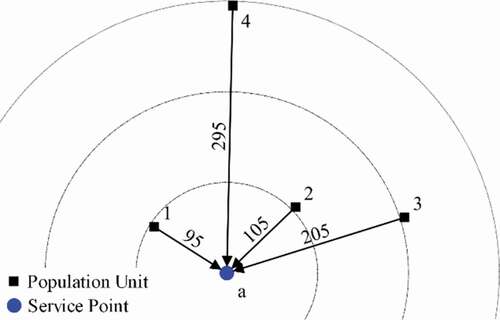
In this setting, a catchment area with a radius of 300 m was defined and divided into three sub-zones of equal size: inner (d_jk ≤ 100 m), central (100 < d_jk ≤ 200 m) and outer (200 m < d_jk ≤ 300 m) sub-zones. The population units 1 and 2 are in the inner and central subzones, respectively, at 95 m and 105 m from a service point, and population units 3 and 4 are in the outer sub-zone at 205 m and 295 m from a service point. The service point ‘a’ is of a capacity of 1, and each population unit consists of 100 people.

2.1. Redefining the travel impedance weights based on fuzzy set theory

Travel impedance weights are redefined based on fuzzy set theory to address the shortcomings of identical accessibility indices within sub-zones and sudden change of accessibility indices across neighbouring sub-zones. Zadeh’s (1965) fuzzy sets allow a member of the universal set to belong with certain grades of membership to more than one subset (or fuzzy set). The grade of membership ranges between 0 and 1. Members of a universal set with grades of 0 are not members of a fuzzy set, and 1 are full members of a fuzzy set. Members of a universal set with grades between 0 and 1 partially belong to a fuzzy set. Hence, a fuzzy set is a list of ordered pairs of objects (elements) and their respective grades of membership:

(3) $F_r=\left\{\left(d_{ij},{\mu }_r\left(d_{ij}\right)\right)\right\},\hspace{0.17em}{d}_{ij}\in \left\{d_{ij}\le d_o\right\}$(3)

where $F_r$ is a fuzzy set (i.e. $r$ is the inner, central or outer sub-zone in the E2SFCA measure), $d_{ij}$ is a travel distance in the E2SFCA measure and a member of a universal set ($d_{ij}\le d_o$), ${\mu }_r\left(d_{ij}\right)$ is a grade of membership of $d_{ij}$ in $F_r$, $d_o$ is the threshold distance.

The degree to which a travel distance belongs to each defined fuzzy set (i.e. the three sub-zones in the E2SFCA measure) is determined by fuzzifying a travel distance using membership functions. The common membership functions used in the fuzzification process include the Gaussian, triangular and trapezoidal membership functions (Kayacan and Khanesar 2016). The non-fuzzy-based Gaussian distance decay function with a downward S-shaped graph is commonly used in FCA measures (Bauer, Groneberg, and Deribe 2016). Therefore, this study adopts the Gaussian membership function (defined by Equation 4)(4) ${\mu }_r\left(\mathrm{x}\right)=e^{-\frac{1}{2}{\left(\frac{x-m}{\sigma }\right)}^2}$(4) for fuzzifying travel distances.

(4) ${\mu }_r\left(\mathrm{x}\right)=e^{-\frac{1}{2}{\left(\frac{x-m}{\sigma }\right)}^2}$(4)

where x is a member of a fuzzy set, m is the centre of a Gaussian membership function and σ is the width of a Gaussian membership function.

Mathematically, the Gaussian membership functions expressed by Equations 5.1(5.1.1) ${\mu }_i\left(d_{1a}\right)=e^{-\frac{1}{2}{\left(\frac{95}{42.466}\right)}^2}=0.0819$(5.1.1) to 5.3(5.3) ${\mu }_o\left(d_{ij}\right)=\left\{\begin{array}{c}{\mathrm{e}}^{-\frac{1}{2}{\left(\frac{d_{ij}-200}{42.466}\right)}^2},100m\le d_{ij}<300m\\ 0,d_{ij}\ge 300m\end{array}\right.$(5.3) determine the degree to which a travel distance belongs to each of the three sub-zones of the hypothetical setting in Figure 1:

(5.1) ${\mu }_i\left(d_{ij}\right)=\left\{\begin{array}{c}{\mathrm{e}}^{-\frac{1}{2}{\left(\frac{d_{ij}}{42.466}\right)}^2},d_{ij}<100m\\ 0,d_{ij}\ge 100m\end{array}\right.$(5.1)

(5.2) ${\mu }_c\left(d_{ij}\right)=\left\{\begin{array}{c}{\mathrm{e}}^{-\frac{1}{2}{\left(\frac{d_{ij}-100}{42.466}\right)}^2},0m<d_{ij}<200m\\ 0,d_{ij}\ge 200m\end{array}\right.$(5.2)

(5.3) ${\mu }_o\left(d_{ij}\right)=\left\{\begin{array}{c}{\mathrm{e}}^{-\frac{1}{2}{\left(\frac{d_{ij}-200}{42.466}\right)}^2},100m\le d_{ij}<300m\\ 0,d_{ij}\ge 300m\end{array}\right.$(5.3)

where ${\mu }_i\left(d_{ij}\right)$, ${\mu }_c\left(d_{ij}\right)$ and ${\mu }_o\left(d_{ij}\right)$ are the grades to which a travel distance $d_{ij}$ in a global catchment area belongs to inner, central and outer subzones, respectively; 0 m, 100 m and 200 m are the centres of the three Gaussian membership functions where $d_{ij}$ 100% belongs to the inner, central and outer sub-zones.

To generate heterogeneous accessibility indices within a sub-zone that gradually change across neighbouring subzones, the grades to which a travel impedance belongs to the three sub-zones are combined using fuzzy set operations. These fuzzy set operations include union (OR), intersection (AND), algebraic product, algebraic sum, arithmetic mean and weighted mean (Rafati and Nikeghbal 2017). The arithmetic and weighted mean are often preferred among these six operations because they allow high grade on one fuzzy set to compensate for low grade on another fuzzy set. The resulting grade becomes higher than the lowest grade and lower than the highest grade (Grabisch, Orlovski, and Yager 1998). However, arithmetic mean operation, in some cases, generates grades of the same value for different travel distances within different sub-zones. For example, assuming population unit 1 in Figure 1 is at 10 m instead of 95 m from service point ‘a’ with grades of 0.8 to inner and 0.2 to central sub-zones, while population unit 2 is at 190 m instead of 105 m from the same service point ‘a’ with grades of 0.2 to central and 0.8 to outer sub-zones, the distances ($d_{1a}$ and $d_{2a}$) from the two population units 1 and 2 to service point ‘a’ are equally weighed with a value of 0.5 obtained by averaging the respective grades. The resulting constant weight of 0.5 for the two different travel distances contradicts with Tobbler’s first law of Geography. Hence, the arithmetic mean operation is not recommended for calculating weights of travel distances based on the grades to which travel distances belong to different sub-zones. On the contrary, the weighted mean fuzzy operation, given by Equation (6)(6) $W_{ij}^f=\frac{{\sum }_{r=1}^n{W}_r{\mu }_r\left(d_{ij}\right)}{{\sum }_{r=1}^n{W}_r}=\frac{W_1{\mu }_1\left(d_{ij}\right)+W_2{\mu }_2\left(d_{ij}\right)+\hspace{0.17em}.\hspace{0.17em}.\hspace{0.17em}.+W_n{\mu }_n\left(d_{ij}\right)}{W_1+W_2+\hspace{0.17em}.\hspace{0.17em}.\hspace{0.17em}.\hspace{0.17em}+W_n}$(6) , addresses the shortcoming of the arithmetic mean fuzzy operation of assigning uniform influence (i.e. weights) to different travel distances from different population units at different sub-zones (Burrough 1989; Grabisch, Orlovski, and Yager 1998).

(6) $W_{ij}^f=\frac{{\sum }_{r=1}^n{W}_r{\mu }_r\left(d_{ij}\right)}{{\sum }_{r=1}^n{W}_r}=\frac{W_1{\mu }_1\left(d_{ij}\right)+W_2{\mu }_2\left(d_{ij}\right)+\hspace{0.17em}.\hspace{0.17em}.\hspace{0.17em}.+W_n{\mu }_n\left(d_{ij}\right)}{W_1+W_2+\hspace{0.17em}.\hspace{0.17em}.\hspace{0.17em}.\hspace{0.17em}+W_n}$(6)

where $W_{ij}^f$ is a grade to which a travel distance $d_{ij}$ belongs to sub-zones (fuzzy sets), called the fuzzy-based travel impedance; $W_r$ is a non-negative weight assigned to a sub-zone $r$; ${\mu }_r\left(d_{ij}\right)$ is a grade to which a travel distance ($d_{ij}$) belongs to a sub-zone $r$.

The weighted mean fuzzy operation addresses the shortcoming of assigning uniform weights to different travel distances by weighing these distances differently based on the grades to which they belong to the sub-zones and the respective influence of such sub-zones (i.e. the respective sub-zones weights). Before utilizing the weighted mean fuzzy operation, the sub-zones are weighed and the travel distances are graded through fuzzification. Based on the same example used for the arithmetic mean fuzzy operation, the weighted mean fuzzy operation assigns a weight of $(0.8W_1+0.2W_2+0W_3)/(W_1+W_2+W_3)$ and $(0W_{1}0.2W_2+0.8W_3)/(W_1+W_2+W_3)$ to $d_{1a}$ and $d_{2a}$, respectively. Using the standardized Luo and Qi (2009) weights (representing a slower distance decay), $W_1$, $W_2$ and $W_3$ of 0.53, 0.36 and 0.11 for inner, central and outer sub-zones, the weights of [(0.8 x 0.53) + (0.2 x 0.36) + (0 x 0.11)]/(0.53 + 0.36 + 0.11) = 0.49 and [(0 x 0.53) + (0.2 x 0.36) + (0.8 x 0.11)]/(0.53 + 0.36 + 0.11) = 0.16 are assigned to $d_{1a}$ and $d_{2a}$, respectively. The resulting weights conform with Tobler’s first law of Geography as higher weight (0.49) is assigned to a much shorter travel distance (10 m) and lower weight (0.16) to a much longer travel distance (190 m). Generally, with the weighted mean fuzzy operation (i.e. Equation 6(6) $W_{ij}^f=\frac{{\sum }_{r=1}^n{W}_r{\mu }_r\left(d_{ij}\right)}{{\sum }_{r=1}^n{W}_r}=\frac{W_1{\mu }_1\left(d_{ij}\right)+W_2{\mu }_2\left(d_{ij}\right)+\hspace{0.17em}.\hspace{0.17em}.\hspace{0.17em}.+W_n{\mu }_n\left(d_{ij}\right)}{W_1+W_2+\hspace{0.17em}.\hspace{0.17em}.\hspace{0.17em}.\hspace{0.17em}+W_n}$(6) ), maximum weights, equalling sub-zones weights, are assigned to travel distances that completely belong to such sub-zones. To completely belong to a sub-zone, a travel distance has to to be of 0 units (i.e. at the service point/centre of the subzone) or a value equalling a distance from the service point to inner boundary of subsequent sub-zones. Thus, travel distances from population units at service point/centre of catchment areas or inner boundary of the subsequent sub-zones are highly weighed. Then, the weights continuously decrease towards outer boundaries of sub-zones with decreasing and increasing influence of highly and lowly weighed sub-zones, respectively. At outer boundaries, weights reach minimum values, equalling the weights of lowly weighed sub-zones; meanwhile, the influence of highly and lowly weighed sub-zones are decreased and increased to 0% and 100%, respectively. In the previous example, the weight assigned to $d_{1a}$ (at 10 m) decreased from 0.53 to 0.49 due to the respective decrease from 0.53 [100% at 0 m (at service point/centre of the catchment area)] to 0.42 (79% at 10 m) and increase from 0 (0% at 0 m) to 0.07 (19% at 10 m) in the influence of the inner and central sub-zones, which are highly and lowly weighed for $d_{1a}$. The weight assigned to $d_{2a}$ (at 190 m) decreased from 0.36 to 0.16 due to the respective decrease from 0.36 [100% at 100 m (the inner boundary of the central zone)] to 0.07[19% at 190 m (near the outer boundary of central sub-zone)] and increase from 0 (0% at 100 m) to 0.09 (82% at 190 m) in the influence of the central and outer sub-zones, which are highly and lowly weighed for $d_{2a}$.

Thus, the fuzzy-based travel distance ($W_{ij}^f$) defined by Equation 6(6) $W_{ij}^f=\frac{{\sum }_{r=1}^n{W}_r{\mu }_r\left(d_{ij}\right)}{{\sum }_{r=1}^n{W}_r}=\frac{W_1{\mu }_1\left(d_{ij}\right)+W_2{\mu }_2\left(d_{ij}\right)+\hspace{0.17em}.\hspace{0.17em}.\hspace{0.17em}.+W_n{\mu }_n\left(d_{ij}\right)}{W_1+W_2+\hspace{0.17em}.\hspace{0.17em}.\hspace{0.17em}.\hspace{0.17em}+W_n}$(6) replaces the travel impedance weights ($W_r$) defined in the E2SFCA measure to account for the influence of differential travel distance within sub-zones. Thus, changing the E2SFCA Equations 1(1) $R_j=\frac{S_j}{D_j}=\frac{S_j}{{\sum }_{k\in \left\{d_{kj}\in D_r\right\}}{P}_k{W}_r}=\frac{S_j}{{\sum }_{k\in \left\{d_{kj}\in D_1\right\}}{P}_k{W}_1+{\sum }_{k\in \left\{d_{kj}\in D_2\right\}}{P}_k{W}_2+.\hspace{0.17em}.\hspace{0.17em}.}$(1) and 2(2) $A_i=\sum _{j\in \left\{d_{ij}\in D_r\right\}}{R}_j{W}_r=\sum _{j\in \left\{d_{ij}\in D_1\right\}}{R}_j{W}_1+\sum _{j\in \left\{d_{ij}\in D_2\right\}}{R}_j{W}_2+.\hspace{0.17em}.\hspace{0.17em}.$(2) into Equations 7(7) $R_j=\frac{S_j}{D_j}=\frac{S_j}{{\sum }_{k\in \left\{d_{kj}\le d_o\right\}}{P}_k{W}_{jk}^f}=\frac{S_j}{P_1{W}_{j1}^f+P_2{W}_{j2}^f+P_3{W}_{j3}^f+\hspace{0.17em}.\hspace{0.17em}.\hspace{0.17em}.}$(7) and 8(8) $A_i=\sum _{j\in \left\{d_{ij}\le d_o\right\}}{R}_j{W}_{ij}^f=R_1{W}_{i1}^f+R_2{W}_{i2}^f+R_3{W}_{i3}^f+\hspace{0.17em}.\hspace{0.17em}.\hspace{0.17em}.$(8) , respectively. Just as with the E2SFCA, the resulting measure called fuzzy-based (F) 2SFCA calculates spatial accessibility indices in two steps. The first step defines catchment areas around supply points, divides them into sub-zones and assigns travel distance weight to each sub-zone. Then, for each travel impedance in a catchment area, a fuzzy-based travel impedance weight is calculated using the weighted mean fuzzy operation. Finally, the supply-to-demand ratio at each supply point is calculated using Equation 7(7) $R_j=\frac{S_j}{D_j}=\frac{S_j}{{\sum }_{k\in \left\{d_{kj}\le d_o\right\}}{P}_k{W}_{jk}^f}=\frac{S_j}{P_1{W}_{j1}^f+P_2{W}_{j2}^f+P_3{W}_{j3}^f+\hspace{0.17em}.\hspace{0.17em}.\hspace{0.17em}.}$(7) :

(7) $R_j=\frac{S_j}{D_j}=\frac{S_j}{{\sum }_{k\in \left\{d_{kj}\le d_o\right\}}{P}_k{W}_{jk}^f}=\frac{S_j}{P_1{W}_{j1}^f+P_2{W}_{j2}^f+P_3{W}_{j3}^f+\hspace{0.17em}.\hspace{0.17em}.\hspace{0.17em}.}$(7)

where $R_j$ is the supply-to-demand ratio at supply point $j$, $S_j$ is the size or capacity of supply point $j$, $D_j$ is the potential demand at supply point $j$, $P_k$ is the population at unit $k$, $d_{kj}$ is a travel impedance between a supply point $j$ and a population unit $k$, $W_{jk}^f$ is a fuzzy-based travel impedance weight assigned to a travel impedance $d_{kj}$ and $d_o$ is the threshold travel impedance that defines the size of a catchment area.

In the second step, catchment areas are defined around population units, divided into sub-zone and each sub-zone is assigned a travel impedance weight. Then, for each travel impedance in a catchment area, a fuzzy-based travel impedance weight is calculated using the weighted mean fuzzy operation. Finally, the spatial accessibility of supply points at population units is calculated using Equation 8(8) $A_i=\sum _{j\in \left\{d_{ij}\le d_o\right\}}{R}_j{W}_{ij}^f=R_1{W}_{i1}^f+R_2{W}_{i2}^f+R_3{W}_{i3}^f+\hspace{0.17em}.\hspace{0.17em}.\hspace{0.17em}.$(8) :

(8) $A_i=\sum _{j\in \left\{d_{ij}\le d_o\right\}}{R}_j{W}_{ij}^f=R_1{W}_{i1}^f+R_2{W}_{i2}^f+R_3{W}_{i3}^f+\hspace{0.17em}.\hspace{0.17em}.\hspace{0.17em}.$(8)

where $A_i$ is the spatial accessibility of supply points at population unit $i$, $R_j$ and $d_o$ are defined as in Equation 6(6) $W_{ij}^f=\frac{{\sum }_{r=1}^n{W}_r{\mu }_r\left(d_{ij}\right)}{{\sum }_{r=1}^n{W}_r}=\frac{W_1{\mu }_1\left(d_{ij}\right)+W_2{\mu }_2\left(d_{ij}\right)+\hspace{0.17em}.\hspace{0.17em}.\hspace{0.17em}.+W_n{\mu }_n\left(d_{ij}\right)}{W_1+W_2+\hspace{0.17em}.\hspace{0.17em}.\hspace{0.17em}.\hspace{0.17em}+W_n}$(6) , $d_{ij}$ is a travel impedance between a population unit $i$ and a supply point $j$ and $W_{ij}^f$ is a fuzzy-based travel impedance weight assigned to a travel impedance $d_{ij}$.

2.2. Implementing E2SFCA and F2SFCA in the hypothetical set up

The step-wise travel impedance weights of 1, 0.68 and 0.22 representing a slower distance decay were adopted from Luo and Qi (2009) and assigned to inner, central and outer sub-zones, respectively. According to the E2SFCA measure, the weights of 1 and 0.68 were assigned to population units 1 and 2 in the inner and central subzones. Regardless of differences in distance, a weight of 0.22 was assigned to population units 3 and 4 in the outer subzone. The supply-to-demand ratio ($R_j$) for service point ‘a’ was calculated using Equation 1(1) $R_j=\frac{S_j}{D_j}=\frac{S_j}{{\sum }_{k\in \left\{d_{kj}\in D_r\right\}}{P}_k{W}_r}=\frac{S_j}{{\sum }_{k\in \left\{d_{kj}\in D_1\right\}}{P}_k{W}_1+{\sum }_{k\in \left\{d_{kj}\in D_2\right\}}{P}_k{W}_2+.\hspace{0.17em}.\hspace{0.17em}.}$(1) :

(1.1) $R_a=\frac{S_a}{D_a}=\frac{S_a}{\left(P_1\times W_1\right)+\left(P_2\times W_2\right)+\left[\left(P_3\times W_3\right)+\left(P_4\times W_3\right)\right]}$(1.1)

(1.2) $R_a=\frac{1}{\left(100\times 1\right)+\left(100\times 0.68\right)+\left[\left(100\times 0.22\right)+\left(100\times 0.22\right)\right]}=0.0047$(1.2)

The population units’ access to service point ‘a’ ($A_i$) based on the E2SFCA measure were calculated using Equation 2(2) $A_i=\sum _{j\in \left\{d_{ij}\in D_r\right\}}{R}_j{W}_r=\sum _{j\in \left\{d_{ij}\in D_1\right\}}{R}_j{W}_1+\sum _{j\in \left\{d_{ij}\in D_2\right\}}{R}_j{W}_2+.\hspace{0.17em}.\hspace{0.17em}.$(2) :

(2.1) $A_1=R_a\times W_1=0.0047\times 1=0.0047$(2.1)

(2.2) $A_2=R_a\times W_2=0.0047\times 0.68=0.0032$(2.2)

(2.3) $A_3=R_a\times W_3=0.0047\times 0.22=0.0010$(2.3)

(2.4) $A_4=R_a\times W_4=0.0047\times 0.22=0.0010$(2.4)

Calculating provider-to-population ratio and accessibility indices according to the F2SFCA measure requires pre-defined fuzzy-based weights, which are determined by fuzzifying travel distance and combining the grades to which travel distances belong to the inner, central and outer sub-zones. From the hypothetical setting in Figure 1, travel distances from population units 1, 2 and 3 to service point ‘a’ are fuzzified using Gaussian membership functions given by Equations 5.1(5.1.1) ${\mu }_i\left(d_{1a}\right)=e^{-\frac{1}{2}{\left(\frac{95}{42.466}\right)}^2}=0.0819$(5.1.1) to 5.3:

(5.1.1) ${\mu }_i\left(d_{1a}\right)=e^{-\frac{1}{2}{\left(\frac{95}{42.466}\right)}^2}=0.0819$(5.1.1)

(5.2.1) ${\mu }_c\left(d_{1a}\right)=e^{-\frac{1}{2}{\left(\frac{95-100}{42.466}\right)}^2}=0.9931$(5.2.1)

(5.2.2) ${\mu }_c\left(d_{2a}\right)=e^{-\frac{1}{2}{\left(\frac{105-100}{42.466}\right)}^2}=0.9931$(5.2.2)

(5.3.1) ${\mu }_o\left(d_{2a}\right)=e^{-\frac{1}{2}{\left(\frac{105-200}{42.466}\right)}^2}=0.0819$(5.3.1)

(5.3.2) ${\mu }_o\left(d_{3a}\right)=e^{-\frac{1}{2}{\left(\frac{205-200}{42.466}\right)}^2}=0.9931$(5.3.2)

(5.3.3) ${\mu }_o\left(d_{4a}\right)=e^{-\frac{1}{2}{\left(\frac{295-200}{42.466}\right)}^2}=0.0819$(5.3.3)

(5.4) ${\mu }_i\left(d_{2a}\right)={\mu }_i\left(d_{3a}\right)={\mu }_i\left(d_{4a}\right)={\mu }_c\left(d_{3a}\right)={\mu }_c\left(d_{4a}\right)={\mu }_o\left(d_{1a}\right)=0$(5.4)

Then, the fuzzy-based weights are determined using Equation 6(6) $W_{ij}^f=\frac{{\sum }_{r=1}^n{W}_r{\mu }_r\left(d_{ij}\right)}{{\sum }_{r=1}^n{W}_r}=\frac{W_1{\mu }_1\left(d_{ij}\right)+W_2{\mu }_2\left(d_{ij}\right)+\hspace{0.17em}.\hspace{0.17em}.\hspace{0.17em}.+W_n{\mu }_n\left(d_{ij}\right)}{W_1+W_2+\hspace{0.17em}.\hspace{0.17em}.\hspace{0.17em}.\hspace{0.17em}+W_n}$(6) ..

(6.1) $W_{1a}^f=\frac{\left(0.0819x1\right)+\left(0.9931x0.68\right)+\left(0x0.22\right)}{1+0.68+0.22}=0.40$(6.1)

(6.2) $W_{2a}^f=\frac{\left(0x1\right)+\left(0.9931x0.68\right)+\left(0.0819x0.22\right)}{1+0.68+0.22}=0.36$(6.2)

(6.3) $W_{3a}^f=\frac{\left(0x1\right)+\left(0x0.68\right)+\left(0.9931x0.22\right)}{1+0.68+0.22}=0.11$(6.3)

(6.4) $W_{4a}^f=\frac{\left(0x1\right)+\left(0x0.68\right)+\left(0.0819x0.22\right)}{1+0.68+0.22}=0.01$(6.4)

Finally, the provider-to-population ratio (R_j) is calculated using Equation 7(7) $R_j=\frac{S_j}{D_j}=\frac{S_j}{{\sum }_{k\in \left\{d_{kj}\le d_o\right\}}{P}_k{W}_{jk}^f}=\frac{S_j}{P_1{W}_{j1}^f+P_2{W}_{j2}^f+P_3{W}_{j3}^f+\hspace{0.17em}.\hspace{0.17em}.\hspace{0.17em}.}$(7) :

(7.1) $R_a=\frac{1}{\left(100x0.4\right)+\left(100x0.36\right)+\left(100x0.11\right)+\left(100x0.01\right)}=0.0114$(7.1)

The population units 1, 2, 3 and 4 access to service point ‘a’ based on the F2SFCA measure are calculated using Equation 8(8) $A_i=\sum _{j\in \left\{d_{ij}\le d_o\right\}}{R}_j{W}_{ij}^f=R_1{W}_{i1}^f+R_2{W}_{i2}^f+R_3{W}_{i3}^f+\hspace{0.17em}.\hspace{0.17em}.\hspace{0.17em}.$(8) :

(8.1) $A_1=0.40x0.0114=0.0045$(8.1)

(8.2) $A_2=0.36x0.0114=0.0040$(8.2)

(8.3) $A_3=0.11\hspace{0.17em}x\hspace{0.17em}0.0114=0.0013\hspace{0.17em}$(8.3)

(8.4) $A_4=0.01x0.0114=0.0001$(8.4)

The resulting E2SFCA and F2SFCA accessibility indices are presented in Figure 2.

Figure 2. Accessibility indices generated by (a) E2SFCA and (b) F2SFCA measures for the hypothetical setup. The upper and lower values at each black squares represent the population units and their respective accessibility indices, and values along the black lines represent the distance in metres from the service point to each population unit.

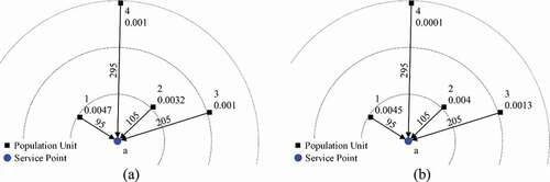
Logically, the accessibility index of population unit 1 is supposed to be closely related to the accessibility index of population unit 2, which is radially 5 m from population unit 1. The accessibility index of population unit 3 is supposed to be quite different from that of population unit 4, which is radially 90 m from population unit 3. On the contrary, in Figure 2(a), the E2SFCA accessibility index of 0.0047 for population unit 1 is greatly different from that of 0.0032 for population unit 2. The E2SFCA accessibility index of 0.0010 is uniform for population units 3 and 4. A large difference in accessibility indices observed between population units 1 and 2, which are close to each other but in two neighbouring sub-zones, and the uniformity in accessibility indices observed within an outer sub-zone reflect the effect of neglecting distance variation within sub-zones.

Contrary to spatial accessibility indices generated by the E2SFCA, spatial accessibility indices generated by the F2SFCA shown in Figure 2(b) vary within each sub-zone and gradually change across neighbouring sub-zones. As expected, the spatial accessibility index at population unit 1 at 95 m in the inner sub-zone is slightly higher than the spatial accessibility index at population unit 2 at 105 m in the central sub-zone. The spatial accessibility index at population unit 3 at 205 m in the outer sub-zone is significantly higher than the spatial accessibility index at population unit 4 at 295 m in the same sub-zone. To a great extent, the spatial accessibility indices generated by the F2SFCA respond according to Tobler’s first law of geography.

3. Implementing F2SFCA in rural wards of Dodoma Urban District

The study tested the proposed F2SFCA method in a GIS environment by calculating the spatial accessibility of water points in the Rural Wards of Dodoma Urban District. It employed two software, QGIS 3.10.5 and IBM Statistics 20, for data processing and analysis.

3.1. Study area and data used

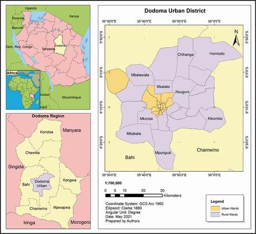
Based on the 2012 administrative boundaries shapefile obtained from the National Bureau of Statistics, the F2SFCA measure was implemented in nine Rural Wards of Dodoma Urban District: Mbalawala, Chihanga, Msalato, Hombolo, Kikombo, Mkonze, Mbabala, Mpunguzi and Nzuguni, shown in Figure3. The 2012 shapefile does not include newly defined administrative boundaries for four Wards, Hombolo Makulu, Hombolo Bwawani, Matumbulu and Mpunguzi. The first two makes the old Hombolo Ward and the last two makes the old Mpunguzi Ward, whereas the old Wards are the ones presented in Figure3. Thus, the study area consists of both the old and new administrative Wards, 11 in total. Dodoma Urban District is a Capital City of Tanzania, with a total population of 410,956 as of the latest census in 2012, of which 197,320 lived in 19 Rural Wards and 213,636 in 18 Urban Wards. The 2016 decision of the fifth Government of Tanzania to run the Capital City in Dodoma Urban District is expected to lead to a rapid population increase with potentially higher demand for water supply. Dodoma Urban District is in the central zone with 9.1% of all water points in Tanzania, significantly less than nearly 20% to around 27% in the other four zones (World Bank 2018). The District is also a semi-arid area with little annual rainfall of about 400 mm to 600 mm falling between December and April. Thus, her inhabitants depend on the groundwater by subscribing to Dodoma Urban Water and Sanitation Authority (DUWASA) or fetching from either community or privately owned water points (i.e. boreholes and shallow wells). However, out of 11 Studied Rural Wards, the DUWASA water supply network partly covers only three Wards: Msalato, Mkonze and Nzuguni.

Based on 70 water points sampled using a two-stage stratified sampling technique from 228 water points available in the 11 Rural Wards, the study defined 19 study zones within these 11 Rural Wards. The study zones enclosed a threshold distance of 400 m from sampled water points that the National Water Policy specifies as an optimal walking distance for a served population (URT, 2002). The defined study zones were coded using three letters followed by four numbers. The three letters and the first two numbers identify a Ward where the study zone is located, and the last two letters identify the study zone in a Ward. For example, SRW1101 is the study zone 01 (identified by the last two letters) in Nzuguni Ward, identified by SRW11. During the field survey, respondents reported an additional 79 water points they preferred, making 149 water points in the 19 study zones, of which six are no longer existing. The capacity of each water point was defined by assigning 1 for functional water points and 0 for non-functional water points in the 19 zones. Given the rural setup of the studied area, all existing buildings in the 19 study zones were digitized in Google Earth to form a household dataset with 5349 households. A household survey was carried out to obtain the household size for 287 (83%) of 344 households sampled from 5349 households. A Voronoi Polygon was created for each surveyed household. Then, the household size of each surveyed household was assigned to the remaining unsurveyed households within the Voronoi polygons where the respective surveyed households are located. Finally, the travel distances from each household to water points within the catchment areas of 400 m (specified in the National Water Policy) were calculated. Figure 3

Figure 3. The study area (i.e. the Labelled Wards) sampled from 19 Rural Wards in Dodoma Urban District.

3.2. Determining F2SFCA accessibility indices in a study area

The F2SFCA spatial accessibility measure was implemented in a GIS environment and involved three procedures: calculating the fuzzy-based weights, provider-to-population ratios and accessibility indices. All calculations were carried out using Field Calculator, Statistics by Categories and Join Attributes by Field Value tools of QGIS 3.10.5 Software.

The proposed F2SFCA measure divides the global catchment area with a radius of 400 m into three subzones of equal size: inner (0 m < $d_{ij}$ < 133 m), central (133 m ≤ $d_{ij}$ < 266 m) and outer (266 m ≤ $d_{ij}$ < 400 m) sub-zones. The lower limits of 0 m, 133 m and 266 m define the centres of the three Gaussian membership functions where a household completely belongs to the inner, central or outer sub-zone. The Gaussian standard deviation (i.e. width) was calculated such that a distance midway between any two neighbouring sub-zones equally belongs to such sub-zones. The centre and standard deviation of the Gaussian membership functions defined in this section [(0, 56.480), (133, 56.480) m and (266, 56.480) m] replaced those in Equations 5.1(5.1.1) ${\mu }_i\left(d_{1a}\right)=e^{-\frac{1}{2}{\left(\frac{95}{42.466}\right)}^2}=0.0819$(5.1.1) to 5.3 [(0, 42.466) m, (100, 42.466) m and (200, 42.466) m]. These new centres and standard deviations were used to calculate the degree of membership to which each travel distance belongs to the inner, central and outer sub-zones. Finally, the degrees of membership to which each travel distance belongs to the inner, central and outer sub-zones were weighted by the respective step-wise weights (i.e. 1, 0.68 and 0.22) and combined using Equation 6(6) $W_{ij}^f=\frac{{\sum }_{r=1}^n{W}_r{\mu }_r\left(d_{ij}\right)}{{\sum }_{r=1}^n{W}_r}=\frac{W_1{\mu }_1\left(d_{ij}\right)+W_2{\mu }_2\left(d_{ij}\right)+\hspace{0.17em}.\hspace{0.17em}.\hspace{0.17em}.+W_n{\mu }_n\left(d_{ij}\right)}{W_1+W_2+\hspace{0.17em}.\hspace{0.17em}.\hspace{0.17em}.\hspace{0.17em}+W_n}$(6) to calculate the fuzzy-based weights.

The potential demand for each water point (i.e. the denominator in Equation 7)(7) $R_j=\frac{S_j}{D_j}=\frac{S_j}{{\sum }_{k\in \left\{d_{kj}\le d_o\right\}}{P}_k{W}_{jk}^f}=\frac{S_j}{P_1{W}_{j1}^f+P_2{W}_{j2}^f+P_3{W}_{j3}^f+\hspace{0.17em}.\hspace{0.17em}.\hspace{0.17em}.}$(7) was calculated by multiplying the household size with the respective fuzzy-based weight to obtain the weighted population. Then, for each water point, the weighted household sizes within the global catchment area with a radius of 400 m were summed up to obtain the potential demand. Finally, for each water point, the water point capacity (i.e. the numerator in Equation 7)(7) $R_j=\frac{S_j}{D_j}=\frac{S_j}{{\sum }_{k\in \left\{d_{kj}\le d_o\right\}}{P}_k{W}_{jk}^f}=\frac{S_j}{P_1{W}_{j1}^f+P_2{W}_{j2}^f+P_3{W}_{j3}^f+\hspace{0.17em}.\hspace{0.17em}.\hspace{0.17em}.}$(7) defined in Section 3.1 was divided by the potential demand (i.e. the denominator in Equation 7)(7) $R_j=\frac{S_j}{D_j}=\frac{S_j}{{\sum }_{k\in \left\{d_{kj}\le d_o\right\}}{P}_k{W}_{jk}^f}=\frac{S_j}{P_1{W}_{j1}^f+P_2{W}_{j2}^f+P_3{W}_{j3}^f+\hspace{0.17em}.\hspace{0.17em}.\hspace{0.17em}.}$(7) to get the water point-to-population ratios.

To calculate accessibility indices, first, the fuzzy-based weight for each travel distance was multiplied by the respective water point-to-population ratio to get the weighted water point-to-population ratios. Finally, for each household, the accessibility index was calculated using Equation 8(8) $A_i=\sum _{j\in \left\{d_{ij}\le d_o\right\}}{R}_j{W}_{ij}^f=R_1{W}_{i1}^f+R_2{W}_{i2}^f+R_3{W}_{i3}^f+\hspace{0.17em}.\hspace{0.17em}.\hspace{0.17em}.$(8) by summing up the weighted water point-to-population ratio within its global catchment area with a radius of 400 m.

3.3. Determining E2SFCA accessibility indices in a study area

The E2SFCA measure was also implemented in a GIS environment to calculate the spatial accessibility of water points in the study area. The implementation of the E2SFCA measure in a GIS environment involved similar procedures followed in the implementation of the F2SFCA measure. However, instead of the fuzzy-based weights, the sub-zone weights of 1, 0.68 and 0.22 were assigned to a distance within the inner, central and outer sub-zone, respectively. Table 1 shows the step-wise and fuzzy-based weights assigned to selected distances in inner, central and outer sub-zones.

Table 1. An extract of step-wise and fuzzy-based weights assigned to three, four and three travel distances from households to water points located in outer, central and inner sub-zones, respectively.

Household	Water point	Travel distance	Sub-zone	Travel distance weights
				Step-wise	Fuzzy-based
MP226	WP0901	386.684	Outer	0.22	0.022
MP231	WP0903	277.115	Outer	0.22	0.216
MP227	WP0901	359.021	Outer	0.22	0.057
MP342	WP0901	264.122	Central	0.68	0.266
MP343	WP0901	235.286	Central	0.68	0.322
MP243	WP0902	206.692	Central	0.68	0.417
MP243	WP0903	133.221	Central	0.68	0.694
MP245	WP0903	111.570	Inner	1.00	0.775
HOM701	WP0502	42.202	Inner	1.00	0.943
MP324	WP0903	131.947	Inner	1.00	0.745

3.4. Assessing the performance of F2SFCA spatial accessibility measure

The performance of the F2SFCA spatial accessibility measure was assessed by comparing the variation of its accessibility indices with the variation of the respective E2SFCA accessibility indices relative to households’ travel distance to water points in the study area. This comparison is made against an accessibility of 0.004, signifying a maximum threshold demand of 250 people per one water point, as specified in the National Water Policy of Tanzania (URT 2002). Thus, an accessibility index of 0.004 corresponds to 100% access to water points by the respective households. The percentage of household members with access to water points was determined by dividing the accessibility indices (F2SFCA and E2SFCA) by 0.004. The resulting proportions (in brackets) were categorized into five classes, namely, no access (0), less than 50% (below 0.5), 50% to less than 100% (0.5 to below 1), 100% to 200% (1 to 2) and above 200% (above 2).

4. Results and discussion

4.1. Comparison of F2SFCA and E2SFCA spatial accessibility indices

The spatial accessibility indices generated by F2SFCA ranges from 0 to 0.3327 with an average of 0.0035 and a standard deviation of 0.0084 water points per person (Table 2). These spatial accessibility indices show that the level of access to water points among households in the study area is not uniform. From Table 2, 1581 households have no access to the available water points, while 1583, 671, 621 and 703 households get access ranging from just above 0% to less than 50%, 50% to less than 100%, 100% to less than 200% and 200% and higher of their demand. On the other hand, the spatial accessibility indices generated by E2SFCA ranges from 0 to 0.3339 with an average of 0.0035 and a standard deviation of 0.0082 water points per person (Table 2). The minimum and mean accessibility indices in F2SFCA and E2SFCA measures are similar, but the maximum and the standard deviation values in F2SFCA are slightly lower and higher than those in the E2FCA.

Table 2. Level of access to water points among households in the 11 Rural Wards of Dodoma Urban District as determined by the F2SFCA and E2SFCA Measures. An accessibility index of 0.004 signifies 100% access to water points by a household as specified by the Tanzania National Water Policy.

Accessibility indices	Households		Population
	F2SFCA	E2SFCA	F2SFCA	E2SFCA
0 (no access)	1581	1581	8646	8646
0–0.0019 (less than 50%)	1583	1550	8059	8062
0.0020–0.0039 (50% to less than 100%)	671	689	3234	3113
0.0040–0.0079 (100% to less than 200%)	621	640	3169	3233
≥0.0080 (200% and above)	703	699	3684	3738

The number of households and population with zero E2SFCA and F2SFCA accessibility indices (i.e. with no access to water points) is the same due to the households located in areas where water points are not functional. The 1583 and 703 households with access less than 50% and greater than 200% in F2SFCA dropped to 1550 and 699 households in E2SFCA. The respective population of 8059 and 3684 increased to 8062 and 3738. On the contrary, households with the access of 50% to less than 100% and 100% to less than 200% increased from 671 and 621 in the F2SFCA to 689 and 640 in the E2SFCA. The respective population dropped from 3234 to 3113 and increased from 3169 to 3233. These observations from the last four rows of Table 2 imply that a household with a higher F2SFCA accessibility index could have a lower E2SFCA accessibility index and vice versa.

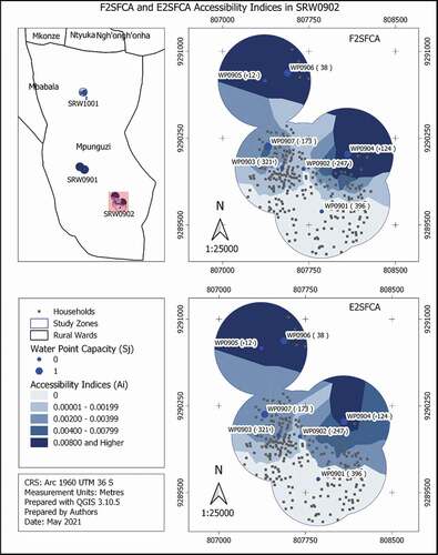
The spatial distribution of households’ F2SFCA and E2SFCA accessibility indices in the study area is visualized in maps created for each study zone. These maps show areas within which households with different levels of accessibility to water points are located.Figure 4, for instance, shows the F2SFCA and E2SFCA accessibility indices for the households in the study zone SRW0902 in Mpunguzi Ward. In Figure 4, the households with no access to water points are in the Southern area of the SRW0902 zone, hosting three water points, which are not functional. Households with the highest F2SFCA and E2SFCA accessibility indices are located in the Northern part of the SRW0902 zone, hosting four water points, of which three are functional and one is not functional. A large proportion of households around functional water points with lower total potential demand have higher F2SFCA and E2SFCA accessibility indices. For example, a large percentage (100%) of households around WP0906 has the highest F2SFCA and E2SFCA accessibility indices, followed by households around WP0904 and WP0907. Both F2SFCA and E2SFCA accessibility indices decrease with an increase in distance from functional water points. Though F2SFCA and E2SFCA accessibility indices exhibit similar patterns, the area with the highest spatial accessibility indices is slightly higher in F2SFCA than in the E2SFCA. The area with lower accessibility indices, ranging between 0.00001 and 0.00200, is much higher in F2SFCA than in the E2SFCA.

Figure 4. F2SFCA and E2SFCA spatial accessibility indices in SRW0902 study zone in Mpunguzi Ward. The grey squares are households, while the blue dots are water points labelled by their ID and total potential demand in the bracket.

The E2SFCA and F2SFCA accessibility indices were further compared graphically using a scatter plot in Figure 5 with the 1:1 reference line, along which households have F2SFCA accessibility indices that equals E2SFCA accessibility indices. Households above a reference line have F2SFCA accessibility indices that are higher than E2SFCA accessibility indices. On the contrary, households below a reference line have F2SFCA accessibility indices that are lower than E2SFCA accessibility indices.

Figure 5. Comparison of the E2SFCA and F2SFCA accessibility indices. Households above and below the red dotted 1:1 reference line have F2SFCA accessibility indices higher and lower than the E2SFCA accessibility indices, respectively.

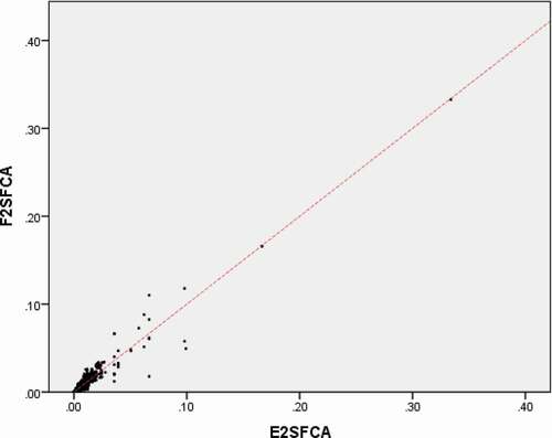
This observation with the real world data conforms to the observation in a hypothetical setup where the resulting F2SFCA accessibility indices were higher than E2SFCA accessibility indices for some households and lower than E2SFCA accessibility indices for other households.

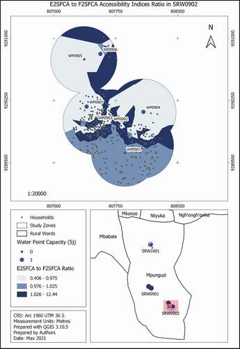
Figure 6 shows areas where F2SFCA accessibility indices are lower than, similar to and higher than the E2SFCA accessibility indices. Areas where the difference in E2SFCA and F2SFCA accessibility indices is within 2.5% (i.e. E2SFCA to F2SFCA ratio is between 0.975 and 1.025) are assumed to have similar accessibility indices. For areas with E2SFCA to F2SFCA ratios below 0.975, their F2SFCA are more than 2.5% less than the E2SFCA accessibility indices. On the other hand, areas with E2SFCA to F2SFCA ratios above 1.025, their F2SFCA are more than 2.5% higher than the E2SFCA accessibility indices. In the SRW0902 study zone (Figure 6), a large proportion of the Northern and Southern parts are characterized with E2SFCA to F2SFCA ratios ranging from 0.406 to 0.974 and 0.976 to 1.025, respectively. In general, 1796 (34%), 1835 (36%) and 1528 (30%) out of 5159 households in the study area have E2SFCA to F2SFCA accessibility indices of 0.974 to 1.025, 0.406 to 0.975 and 1.026 to 12.44. This implies that more households (exceeding by 4%) have better spatial access to water points with F2SFCA measure than E2SFCA measure.

Figure 6. Ratios of E2SFCA to F2SFCA accessibility indices in SRW0902, Mpunguzi Ward, signifying areas where F2SFCA accessibility indices are higher, similar and lower than E2SFCA accessibility indices for each household.

4.2. The performance of F2SFCA spatial accessibility measure at the household level

The F2SFCA and E2SFCA spatial accessibility indices for individual households are presented in Figure 7.

Figure 7. F2SFCA and E2SFCA spatial accessibility indices. The black squares are households with their ID and size in the bracket, F2SFCA indices and E2SFCA indices shown by the upper, middle and lower labels, respectively. The blue dots are water points labelled with their ID. The regions where households are within the same sub-zones (i.e. accessing the same water points) are shown by different colours and identified by capital letters.

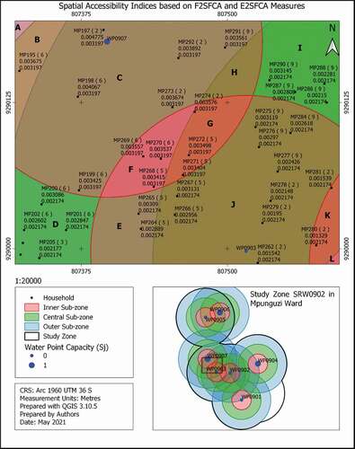
The F2SFCA accessibility indices vary from one household to another within and across sub-zones. For example, the households within region C in Figure 7 formed by an intersection of the inner, central and outer sub-zones of water points’ WP0907, WP0903 and WP0902 catchment areas have different F2SFCA spatial accessibility indices. Since households within each region are in the same sub-zones, they are accessing the same water points. Thus, the variation in their F2SFCA spatial accessibility indices is due to the variation in their travel distances. Households closer to functional water points with high levels of service have higher F2SFCA spatial accessibility indices. For instance, in Figure 7, F2SFCA spatial accessibility indices are higher for households closer to functional water point WP0907 and decrease towards non-functional water points WP0903 and WP0902. This variation in the F2SFCA accessibility indices is observed throughout the study area. Unlike F2SFCA, E2SFCA accessibility indices (the lower household labels) vary for households within different regions but are uniform for households within the same region. For example, households in region C have identical E2SFCA spatial accessibility indices of 0.003197. Since only WP0907 is functional in Figure 7, households in each sub-zone around WP0907 but different regions have identical E2SFCA spatial accessibility indices. This means the uniformity in the E2SFCA spatial accessibility indices extends from one region to another region. For example, the identical E2SFCA spatial accessibility indices of 0.003197 in region C has also been observed in regions B, F and G. This uniformity in E2SFCA accessibility indices has been observed for both individual and set of regions throughout the study area. The observed variation in F2SFCA and uniformity in E2SFCA accessibility indices in each region in a study area is similar to what was observed in a hypothetical setup in Section 2.2. Similar to the hypothetical setup, the E2SFCA accessibility indices for households close to each other but in different regions are quite different, while the F2SFCA accessibility indices are closely related. For example, a household MP199 in region C near the boundary with region D has the E2SFCA accessibility index of 0.003197, identical to another household MP197 (which is in the same region C and very far), but very different to MP200 (which is in region D but very close) that has the E2SFCA accessibility index of 0.002174. On the contrary, the F2SFCA accessibility indices (in the brackets) for MP199 (0.003425) and MP197 (0.004775) in region C but far from each other are quite different, but for MP199 (0.003425) and MP200 (0.003086) in different regions but close to each other are closely related. These variations in E2SFCA and F2SFCA accessibility indices are also observed in different regions and across different neighbouring regions (e.g. between regions E and F and regions G and J).

Compared to E2SFCA, FSSFCA accessibility indices are more representative of the reality as they reflect distance variation among households to a greater extent and vary according to Tobler’s first law of Geography. This kind of variation in F2SFCA accessibility indices is also observed in other studies employing different continuous travel impedance functions (Bauer, Groneberg, and Deribe 2016; Dai and Wang 2011; Subal, Paal, and Krisp 2021; Z. Xia et al. 2019). For example, Bauer, Groneberg, and Deribe (2016) developed a variable distance decay function based on the median and standard deviation of all population-to-provider distance within the global catchment size and applied it in a case study of the metropolitan area of Berlin, Germany. As F2SFCA, Bauer, Groneberg, and Deribe’s (2016) resulting spatial accessibility indices for both theoretical and a case study area reflected the individual travel behaviour determined by the distribution of providers.

According to Subal, Paal, and Krisp (2021), the spatial accessibility indices resulting from all FCA methods increases with a higher number of supply locations and a higher capacity, a lower amount of demand and increasing proximity of supply to demand locations. However, in Figure 7, regardless of the variation in household size, the E2SFCA spatial accessibility indices are identical in each region. Since the F2SFCA method determines the potential demand similar to the E2SFCA measure as the total potential demand for each water point, the resulting variation in F2SFCA accessibility indices in each region is attributed to the variation in the travel distance and not in the households’ size. Unlike the studies done by W. Luo and Qi (2009) and McGrail (2012), which tested the sensitivity of the E2SFCA measure to different travel impedance coefficients, this study does not test the sensitivity of the F2SFCA measure to different fuzzy membership functions because the step-wise weights employed in the existing measures are based on the Gaussian impedance decay functions.

5. Conclusion

This study proposes an approach for defining continuous travel impedance weights in fFCA measures based on previous research. The study uses the hypothetical setup of one service point and four consumers to illustrate the theoretical limitation of the subzones’ discrete weights in the E2SFCA measure. The study further illustrates the potential of using fuzzy functions in defining different weights for different travel distances within sub-zones based on their degrees of membership to different sub-zones and sub-zones’ discrete weights. The resulting spatial accessibility measure, the fuzzy-based (F) 2SFCA, was applied in the hypothetical setup and tested in the real world by calculating households’ spatial access to water points in Dodoma Rural Wards. Compared to the E2SFCA, the F2SFCA spatial accessibility measure provides a realistic characterization of households’ spatial accessibility of water points, reflecting distance heterogeneity in sub-zones and gradual change in accessibility indices across sub-zone boundaries. Thus, the resulting F2SFCA accessibility indices could be useful in tracking the progress made in improving accessibility of services and planning for allocating new service facilities. The F2SFCA measure could also be applied in assessing the accessibility of facilities and amenities outside the water sector. The observed variation in F2SFCA accessibility indices is due to heterogeneity in water points’ total potential demand and travel distance but not the heterogeneity in local demand. Also, as the study was based on W. Luo and Qi’s (g2009) step-wise weights derived from the Gaussian decay function, only the Gaussian fuzzy membership function was employed without checking the sensitivity of the F2SFCA measure to different fuzzy membership functions. Thus, future works could be directed towards modelling the heterogeneity in local demand to get spatial accessibility indices that vary with service points’ total potential demand, travel distance and service users’ local demand.

Acknowledgements

The authors thank the University of Dodoma for funding this research, Directorate of Rural Water Supply of Tanzania for providing water point data through the Government Basic Statistics Portal; the National Bureau of Statistics for the 2012 shapefiles of administrative boundaries and the QGIS Development team for a free and open-source GIS application, QGIS 3.10.5, employed in this study.

Disclosure statement

No potential conflict of interest was reported by the author(s).

Data availability statement

Data used in this study include shapefile of administrative boundaries (i.e. Dodoma Urban District and Wards shapefile) obtained from the National Bureau of Statistics (NBS) of Tanzania through https://www.nbs.go.tz/index.php/en/census-surveys/gis/386-2012-phc-shapefiles-level-three; water point data obtained from the Directorate of Rural Water Supply (DRWS) of Tanzania through the Government Basic Statistics Portal; Study zones derived using water point data as input and a buffer tool of QGIS 3.10.5 software; and households data obtained from Google Earth through digitization household survey. The study zones, and household data with F2SFCA and E2SFCA accessibility indices are available in Mendeley data repository via DOI:10.17632/6vvsd7778z.1.

Additional information

Funding

This study was funded by the University of Dodoma as part of the PhD research.

References

- Bauer, J., D. Klingelhöfer, W. Maier, L. Schwettmann, and D. A. Groneberg. 2020. “Prediction of Hospital Visits for the General Inpatient Care Using Floating Catchment Area Methods: A Reconceptualization of Spatial Accessibility.” International Journal of Health Geographics 19 (29). doi:10.1186/s12942-020-00223-3.
- Bauer, J., D. A. Groneberg, and K. Deribe. 2016. “Measuring Spatial Accessibility of Health Care Providers-introduction of a Variable Distance Decay Function within the Floating Catchment Area (FCA) Method.” PLoS ONE 11 (7): e0159148. doi:10.1371/journal.pone.0159148.
- Bozorgi, P., J. M. Eberth, J. P. Eidson, and D. E. Porter. 2021. “Facility Attractiveness and Social Vulnerability Impacts on Spatial Accessibility to Opioid Treatment Programs in South Carolina.” International Journal of Environmental Research and Public Health 18 (4246): 4246. doi:10.3390/ijerph18084246.
- Bryant, J., Jr, and P. L. Delamater. 2019. “Annals of GIS Examination of Spatial Accessibility at Micro- and Macro-levels Using the Enhanced Two-step Floating Catchment Area (E2SFCA) Method.” Annals of GIS 25 (3): 219–229. doi:10.1080/19475683.2019.1641553.
- Burrough, P. 1989. “Fuzzy Mathematical Methods for Soil Survey and Land Evaluation.” Journal of Soil Science 40 (3): 477–492. doi:10.1111/j.1365-2389.1989.tb01290.x.
- Chen, X. 2019. “Enhancing the Two-Step Floating Catchment Area Model for Community Food Access Mapping: Case of the Supplemental Nutrition Assistance Program.” Professional Geographer 71 (4): 668–680. doi:10.1080/00330124.2019.1578978.
- Cheng, L., M. Yang, J. De Vos, and F. Witlox. 2020. “Examining Geographical Accessibility to Multi-tier Hospital Care Services for the Elderly: A Focus on Spatial Equity.” Journal of Transport and Health 19 (August): 100926. doi:10.1016/j.jth.2020.100926.
- Dai, D., and F. Wang. 2011. “Geographic Disparities in Accessibility to Food Stores in Southwest Mississippi.” Environment and Planning. B, Planning & Design 38 (4): 659–677. doi:10.1068/b36149.
- Delamater, P. L. 2013. “Spatial Accessibility in Suboptimally Configured Health Care Systems: A Modified Two-step Floating Catchment Area (M2SFCA) Metric.” Health & Place 24: 30–43. doi:10.1016/j.healthplace.2013.07.012.
- Freeman, V. L., K. B. Naylor, E. E. Boylan, B. J. Booth, O. Pugach, R. E. Barrett, R. T. Campbell, and S. L. McLafferty. 2020. “Spatial Access to Primary Care Providers and Colorectal Cancer-specific Survival in Cook County, Illinois.” Cancer Medicine 9 (9): 3211–3223. doi:10.1002/cam4.2957.
- Ghorbanzadeh, M., K. Kim, E. Erman Ozguven, and M. W. Horner. 2021. “Spatial Accessibility Assessment of COVID-19 Patients to Healthcare Facilities: A Case Study of Florida.” Travel Behaviour and Society 24: 95–101. doi:10.1016/j.tbs.2021.03.004.
- Grabisch, M., S. A. Orlovski, and R. R. Yager. 1998. “Fuzzy Aggregation of Numerical Preferences.” In Fuzzy Sets in Decision Analysis, Operations Research and Statistics, edited by R. Słowiński, 31–68, Boston, MA: Springer Science+Business Media.
- Guagliardo, M. F. 2004. “Spatial Accessibility of Primary Care: Concepts, Methods and Challenges.” International Journal of Health Geographics 3 (3): 3. doi:10.1186/1476-072X-3-3.
- Hansen, W. G. 1959. “Journal of the American Institute of Planners.” Journal of American Institute of Planners 25 (2): 73–76. doi:10.1080/00049999.1976.9656483.
- Hu, S., W. Song, C. Li, and J. Lu. 2020. “A Multi-mode Gaussian-based Two-step Floating Catchment Area Method for Measuring Accessibility of Urban Parks.” Cities 105: 102815. doi:10.1016/j.cities.2020.102815.
- Joseph, A. E., and P. R. Bantock. 1982. “Measuring Potential Physical Accessibility to General Practitioners in Rural Areas: A Method and Case Study.” Social Science & Medicine 16 (1): 85–90. doi:10.1016/0277-9536(82)90428-2.
- Kar, A., N. Wan, T. J. Cova, H. Wang, and S. L. Lizotte. 2021. “Using GIS to Understand the Influence of Hurricane Harvey on Spatial Access to Primary Care.” Risk Analysis. doi:10.1111/risa.13806.
- Kayacan, E., and M. A. Khanesar. 2016. “Fundamentals of Type-1 Fuzzy Logic Theory.” In Fuzzy Neural Networks for Real Time Control Applications, edited by K. Erdal, and A. K. Mojtaba, 13–24. Oxford: Butterworth-Heinemann. doi:10.1016/b978-0-12-802687-8.00002-5.
- Kiani, B., A. Mohammadi, R. Bergquist, and N. Bagheri. 2021. “Different Configurations of the Two-step Floating Catchment Area Method for Measuring the Spatial Accessibility to Hospitals for People Living with Disability: A Cross-sectional Study.” Archives of Public Health 79 (85). doi:10.1186/s13690-021-00601-8.
- Kim, K., M. Ghorbanzadeh, M. W. Horner, and E. E. Ozguven. 2021. “Identifying Areas of Potential Critical Healthcare Shortages: A Case Study of Spatial Accessibility to ICU Beds during the COVID-19 Pandemic in Florida.” Transport Policy 110: 478–486. doi:10.1016/j.tranpol.2021.07.004.
- Li, M., M. P. Kwan, J. Chen, J. Wang, J. Yin, and D. Yu. 2021. “Measuring Emergency Medical Service (EMS) Accessibility with the Effect of City Dynamics in a 100-year Pluvial Flood Scenario.” Cities 117: 103314. doi:10.1016/j.cities.2021.103314.
- Lin, Y., N. Wan, S. Sheets, X. Gong, and A. Davies. 2018. “A Multi-modal Relative Spatial Access Assessment Approach to Measure Spatial Accessibility to Primary Care Providers.” International Journal of Health Geographics 33. doi:10.1186/s12942-018-0153-9.
- Liu, S., Y. Wang, D. Zhou, and Y. Kang. 2020. “Two-step Floating Catchment Area Model-based Evaluation of Community Care Facilities’ Spatial Accessibility in Xi’an, China.” International Journal of Environmental Research and Public Health 17 (14): 1–17. doi:10.3390/ijerph17145086.
- Luo, J. 2014. “Integrating the Huff Model and Floating Catchment Area Methods to Analyze Spatial Access to Healthcare Services.” Transactions in GIS 18 (3): 436–448. doi:10.1111/tgis.12096.
- Luo, J. 2016. “Analyzing Potential Spatial Access to Primary Care Services with an Enhanced Floating Catchment Area Method.” Cartographica 51 (1): 12–24. doi:10.3138/cart.51.1.3230.
- Luo, W., and Y. Qi. 2009. “An Enhanced Two-step Floating Catchment Area (E2SFCA) Method for Measuring Spatial Accessibility to Primary Care Physicians.” Health & Place 15 (4): 1100–1107. doi:10.1016/j.healthplace.2009.06.002.
- Luo, W., and F. Wang. 2003. “Measures of Spatial Accessibility to Health Care in a GIS Environment: Synthesis and a Case Study in the Chicago Region.” Environment and Planning. B, Planning & Design 30 (6): 865–884. doi:10.1068/b29120.
- Luo, W., and T. Whippo. 2012. “Variable Catchment Sizes for the Two-step Floating Catchment Area (2SFCA) Method.” Health & Place 18 (4): 789–795. doi:10.1016/j.healthplace.2012.04.002.
- Mahuve, F., E. Liwa, and J. Chaula. 2015. “Assessment of Spatial Accessibility to Health Care Facilities in Tanzania: A Case of Wanging’ombe District in Njombe Region.” The Journal of Building and Land Development 18 (1 & 2): 125–137. https://www.ajol.info/index.php/jbld/article/view/178232.
- McGrail, M. R. 2012. “Spatial Accessibility of Primary Health Care Zutilizing the Two Step Floating Catchment Area Method: An Assessment of Recent Improvements.” International Journal of Health Geographics 11 (50): 50. doi:10.1186/1476-072X-11-50.
- Mohammadi, A., A. Mollalo, R. Bergquist, and B. Kiani. 2021. “Measuring COVID-19 Vaccination Coverage: An Enhanced Age-adjusted Two-step Floating Catchment Area Model.” Infectious Diseases of Poverty 10 (118). doi:10.1186/s40249-021-00904-6.
- Ni, J., M. Liang, Y. Lin, Y. Wu, and C. Wang. 2019. “Multi-mode Two-step Floating Catchment Area (2SFCA) Method to Measure the Potential Spatial Accessibility of Healthcare Services.” ISPRS International Journal of Geo-Information 8 (5): 236. doi:10.3390/ijgi8050236.
- Paez, A., C. D. Higgins, S. F. Vivona, and T. I. Shah. 2019. “Demand and Level of Service Inflation in Floating Catchment Area (FCA) Methods.” PLoS ONE 14 (6): e0218773. doi:10.1371/journal.pone.0218773.
- Peng, T. C. 2020. “The Capitalization of Spatial Healthcare Accessibility into House Prices in Taiwan: An Application of Spatial Quantile Regression.” International Journal of Housing Markets and Analysis. doi:10.1108/IJHMA-06-2020-0076.
- Radke, J., and L. Mu. 2000. “Spatial Decompositions, Modeling and Mapping Service Regions to Predict Access to Social Programs.” Geographic Information Sciences 6 (2): 105–112. doi:10.1080/10824000009480538.
- Rafati, S., and M. Nikeghbal. 2017. “Groundwater Exploration Using Fuzzy Logic Approach in GIS for an Area around an Anticline, Fars Province.” The International Archives of the Photogrammetry, Remote Sensing and Spatial Information Sciences XLII (4/W4): 441–445. doi:10.5194/isprs-archives-XLII-4-W4-441-2017.
- Schuurman, N., M. Bérubé, and V. A. Crooks. 2010. “Measuring Potential Spatial Access to Primary Health Care Physicians Using a Modified Gravity Model.” Canadian Geographer 54 (1): 29–45. doi:10.1111/j.1541-0064.2009.00301.x.
- Shaw, S., and H. Sahoo. 2020. “Accessibility to Primary Health Centre in a Tribal District of Gujarat, India: Application of Two Step Floating Catchment Area Model.” GeoJournal 85 (2): 505–514. doi:10.1007/s10708-019-09977-1.
- Stewart, K., M. Li, Z. Xia, S. A. Adewole, O. Adeyemo, and C. Adebamowo. 2020. “Modeling Spatial Access to Cervical Cancer Screening Services in Ondo State, Nigeria.” International Journal of Health Geographics 19 (28). doi:10.1186/s12942-020-00222-4.
- Su, H., W. Chen, and M. Cheng. 2021. “Using the Variable Two-step Floating Catchment Area Method to Measure the Potential Spatial Accessibility of Urban Emergency Shelters.” GeoJournal 3. doi:10.1007/s10708-021-10389-3.
- Subal, J., P. Paal, and J. M. Krisp. 2021. “Quantifying Spatial Accessibility of General Practitioners by Applying a Modified Huff Three ‑ Step Floating Catchment Area (MH3SFCA) Method.” International Journal of Health Geograp. International Journal of Health Geographics 20 (9). doi:10.1186/s12942-021-00263-3.
- Tao, Z., Y. Cheng, S. Du, L. Feng, and S. Wang. 2020. “Accessibility to Delivery Care in Hubei Province, China.” Social Science & Medicine 260: 113186. doi:10.1016/j.socscimed.2020.113186.
- Tao, Z., Z. Yao, H. Kong, F. Duan, and G. Li. 2018. “Spatial Accessibility to Healthcare Services in Shenzhen, China: Improving the Multi-modal Two-step Floating Catchment Area Method by Estimating Travel Time via Online Map APIs.” BMC Health Services Research 18 (345). doi:10.1186/s12913-018-3132-8.
- Tobler, W. R. 1970. “A Computer Movie Simulation Urban Growth in Detroit Region.” Economic Geography 46: 234–240. doi:10.1126/science.11.277.620.
- United Republic of Tanzania. 2002. “Tanzanian Water Policy.”
- Wan, N., B. Zou, and T. Sternberg. 2012. “A Three-step Floating Catchment Area Method for Analyzing Spatial Access to Health Services.” International Journal of Geographical 26 (6): 1073–1089. doi:10.1080/13658816.2011.624987.
- Wang, F., and W. Luo. 2005. “Assessing Spatial and Nonspatial Factors for Healthcare Access: Towards an Integrated Approach to Defining Health Professional Shortage Areas.” Health & Place 11 (2): 131–146. doi:10.1016/j.healthplace.2004.02.003.
- World Bank. 2018. “Reaching for the SDGs: The Untapped Potential of Tanzanias Water Supply, Sanitation, and Hygiene Sector.” In WASH Poverty Diagnosis, 165. Washington, DC: World Bank.
- Wu, H., L. Liu, Y. Yu, and Z. Peng. 2018. “Evaluation and Planning of Urban Green Space Distribution Based on Mobile Phone Data and Two-step Floating Catchment Area Method.” Sustainability (Switzerland) 10 (1). doi:10.3390/su10010214.
- Xiao, W., Y. D. Wei, and N. Wan. 2021. “Modeling Job Accessibility Using Online Map Data: An Extended Two-step Floating Catchment Area Method with Multiple Travel Modes.” Journal of Transport Geography 93: 103065. doi:10.1016/j.jtrangeo.2021.103065.
- Zadeh, L. 1965. “Fuzzy Sets.” Information and Control 8 (3): 338–353. doi:10.1061/9780784413616.194.
- Zahnd, W. E., M. J. Josey, M. Schootman, and J. M. Eberth. 2021. “Spatial Accessibility to Colonoscopy and Its Role in Predicting Late-stage Colorectal Cancer.” Health Services Research 56 (1): 73–83. doi:10.1111/1475-6773.13562.
- Zheng, Z., W. Shen, Y. Li, Y. Qin, and L. Wang. 2020. “Spatial Equity of Park Green Space Using KD2SFCA and Web Map API: A Case Study of Zhengzhou, China.” Applied Geography 123: 102310. doi:10.1016/j.apgeog.2020.102310.
- Zhou, Y., K. M. M. Beyer, P. W. Laud, A. N. Winn, L. E. Pezzin, A. B. Nattinger, and J. Neuner. 2021. “An Adapted Two-step Floating Catchment Area Method Accounting for Urban–rural Differences in Spatial Access to Pharmacies.” Journal of Pharmaceutical Health Services Research 12 (1): 69–77. doi:10.1093/jphsr/rmaa022.
- Zhu, L., S. Zhong, W. Tu, J. Zheng, S. He, J. Bao, and C. Huang. 2019. “Assessing Spatial Accessibility to Medical Resources at the Community Level in Shenzhen, China.” International Journal of Environmental Research and Public Health 16 (242): 242. doi:10.3390/ijerph16020242.
- Xia, T., X. Song, H. Zhang, X. Song, H. Kanasugi, and R. Shibasaki. 2019a. “Measuring Spatio-temporal Accessibility to Emergency Medical Services through Big GPS Data.” Health & Place 56: 53–62. doi:10.1016/j.healthplace.2019.01.012.
- Xia, Z., H. Li, Y. Chen, and W. Yu. 2019b. “Integrating Spatial and Non-spatial Dimensions to Measure Urban Fire Service Access.” ISPRS International Journal of Geo-Information 8 (3): 138. doi:10.3390/ijgi8030138.