Modelling full-colour images of Earth: simulation of radiation brightness field of Earth’s atmosphere and underlying surface

ABSTRACT

This article is dedicated to the problem of realistic colour rendering of space object images using the tools of computer graphics. In the form of a short essay, the authors describe the essence, sources and functionality of modern graphics applications. Particular attention is paid to the application of modern graphics in space science. The specific purpose of the study is the use of computer graphics in the field of remote sensing of the Earth’s surface. This article describes a method for synthesizing images to develop realistic 3D models of colour Earth images in the visible spectral range, observed from geostationary orbits. The method is based on the improved model of atmospheric radiation for arbitrary sighting conditions in an inhomogeneous spherical atmosphere. Physical models of horizontally inhomogeneous distributions of atmospheric density, temperature and albedo of the Earth were improved. All calculations were performed in accordance with the model of molecular scattering of radiation in a spherical atmosphere, taking into account sunlight forward-scattering and reflection from the planet’s surface. This allows us to obtain images of the Earth in its various phases, observed from arbitrary heights. The obtained theoretical colour images of the Earth were compared with black and white images from modern geostationary satellites.

KEYWORDS:

• Albedo
• the earth colour images
• earth’s atmosphere
• satellite
• geostationary orbits

1. Introduction

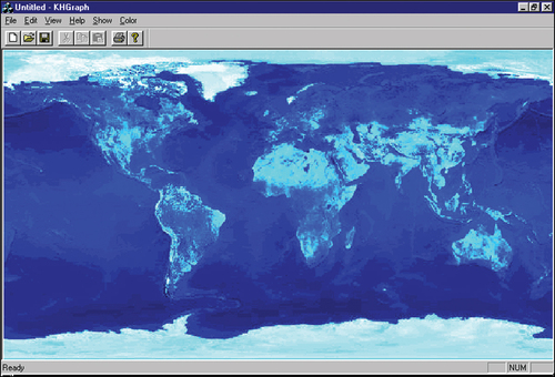
Methods of remote sensing of the Earth’s surface, the use of which began in the 1960s with the launch of artificial space satellites, led to a real technical revolution in many disciplines of Earth sciences (Rodionov et al. 2020; Koteleva and Frenkel 2021). Their use made it possible to assess the planetary distribution of different natural objects and processes, as well as anthropogenic impact on the environment, in order to solve various fundamental and applied problems of natural sciences. The first and most widely used method of remote sensing is taking photographs of the Earth’s surface and the cloud cover in the visible spectrum. At the same time, the beginning of the space era was marked by rapid development of computer graphics, stimulated by successful transition from mechanical calculators to electronic computers. A brief historical overview of the development of computer graphics in terms of Earth imaging is presented in Appendix A.

1.1 Studies of natural phenomena and computer graphics

Image synthesis for realistic 3D model elaboration is one of the most popular areas of relevant research studies (Zotti 2007; Chepyzhova, Pravdina, and Lepikhina 2019). In this way, we obtained colourful images of natural objects, such as mountains, trees, sea, clouds and the Earth images (Figure 2) as well (Preetham, Shirley, and Smits 1999). The images are widely used in movies or commercial TV shows like CG Earth Images library (Shutterstock 2020). However, here they mostly strove to get realistic images, not physically relevant ones.

Figure 1. Block structure of the spherical model of Rayleigh radiation brightness in the atmosphere.

Image synthesis is used to simulate the structure views of building and urban area (Kaneda et al. 1991; HosseiniHaghighi et al. 2020) scenery under various atmospheric conditions, fog views in various sunlight and colours of sunset and dawn (Klassen 1987). Synthesis is also applicable for the calculation models comparison intended to predict daily variations of sky lighting for the energy saving tasks (HosseiniHaghighi et al. 2020; Littlefair 1994). These papers show the image synthesis considering atmospheric influence, but single-scattering approximation only.

Meanwhile, in our opinion, for perfect Earth image modelling, resembling the observations from meteorological satellites, and for their association with weather models, in this case, they can be used to study climate changes, as well as for space flight simulation, it is necessary to have physically based images that require multiple scattering. The subject was studied and described in few papers (Nishita et al. 1996; Tomoyuki et al. 1993; Nishita and Dobashi 2001). The authors of these articles showed detailed images of the landscape and the sea, but the scope of data on the sunlight diffused in the atmosphere and re-reflected by the Earth’s surface (diffuse component) was not considered. Moreover, the non-homogeneous nature of temperature distribution and the Earth’s albedo, affecting the geographical distribution of high-altitudinal atmospheric density changes, were not considered as well.

It should be noted that the synthesis of various natural phenomena and scene images is carried out mainly by digital artists; therefore, the atmospheric models’ reality is rather neglected, with the consequential impact on the research results.

At the same time, the experts on atmospheric optics provide their results in graphical or tabular form, using numerous atmospheric and meteorological parameters that are poorly controlled in experiments. This is why it is difficult and sometimes even impossible to compare these data with a large scope of data obtained from modern space experiments, presented as images.

1.2 The role of optical models in the visualization of natural phenomena

Further development of technologies for photo and video recording made it possible to replace black-and-white representations of captured objects with colour ones, photo and video films – with carriers of digital information, as well as significantly increase the resolving power of camera lenses. Colour images of the underlying surface acquired special importance in this process. They made it possible to assess distribution areas of surface water masses and zones of biological productivity in the World Ocean and to determine various details of terrestrial landscapes in a very wide colour spectrum. Now the largest image area of the underlying Earth’s surface can be obtained from satellites in geostationary orbits.

Various computer programs help to increase the processing speed of colour digital information, but their algorithms are mostly based on principles (parallel computing and delays in individual tasks) that do not provide in the visible spectrum an objective picture of realistic colour rendering for natural objects и явлений.

This is largely due to the shift in microprocessors from single-core to multi-core chips. This trend, most evident in CPU families, aims to run parallel workloads. This maximizes overall throughput although it may be necessary to sacrifice the sequential performance of a single task and the impact of the light transmission functions of Earth’s atmosphere by photo and video cameras.

This is largely due to the influence of light transmission of photo and video cameras through the Earth’s atmosphere. These functions are characterized by strong fluctuations in the three-dimensional plane of the Earth’s surface, as well as in the time range of their seasonal and synoptic-scale variations.

The MODTRAN (atmospheric transmittance/radiation with moderate resolution) software in different versions is currently especially popular. The first version of this program was published in 1987 (Berk, Bernstein, and Robertson MODTRAN 1987). Related subroutines were integrated into LOWTRAN 6. The spectral resolution of this new option exceeds 5 cm⁻¹ (FWHM). The focus is on FASCOD (Fast Atmospheric Signature Code) calculations with the HITRAN (High-Resolution Transmission) molecular spectroscopy spectral database (Rothman et al. 2013). It presents a collection of spectroscopic parameters used to model and analyse the transmission and emission of light in the gas atmospheres of the planet.

The first LOWTRAN programs, which preceded the MODTRAN series and appeared simultaneously with the personal computers in the early seventies, were semi-empirical. A LOWTRAN 3 (see reference 3 in Selby and A 1975) computer program is described for calculating the transmittance of the atmosphere in the spectral region from 0.25 to 28.5 micrometres at a spectral resolution of 20 cm⁻¹. The program provides a choice of six atmospheric models covering seasonal and latitudinal variations from the sea level to 100 km, two haze models, and accounts for molecular absorption, molecular scattering and aerosol extinction. Refraction and earth curvature effects are also included. This program provides some modifications to the molecular absorption and aerosol extinction data provided in an earlier LOWTRAN 2 report. In addition, input modifications have been made, making the LOWTRAN 3 program considerably more flexible in terms of the input of meteorological data.

LOWTRAN 7 is a low-resolution spreading model (Kneizys, Eric Shettle, and Chetwynd 1988) and simultaneously a computer code for predicting atmospheric transmittance and background radiation from 0 to 50,000 cm⁻¹ at 20 cm⁻¹ resolution. The code is based on the LOWTRAN 6 model (Kneizys et al. 1983). Multiple scattered radiation has been added to the model, as well as new molecular band model parameters and new ozone and molecular oxygen absorption parameters for the UV radiation. Other modifications include a wind-dependent desert model and new models of cirrus clouds, clouds and rain.

The SENTRAN computer code, originally developed by researchers at the University of Pennsylvania, is worth noting. It allows users to quickly estimate transmittance and emission from LOWTRAN in response to perturbations of input atmospheric conditions. The code provides a convenient and efficient interface for creating multiple LOWTRAN input decks as well as a graphical representation of the output data in 2D and 3D formats. The main purpose of this paper is to update the SENTRAN source code for use with LOWTRAN7 (Longtin et al. 1991) as well as MODTRAN (Longtin and Hummel 1993).

The MODTRAN computer code series is now used worldwide by researchers and scientists in government agencies, commercial organizations and educational institutions to predict and analyse optical measurements through the atmosphere. The code is integrated into many operational and research sensor and data processing systems. They are commonly referred to as atmospheric correction in remotely sensed multispectral and hyperspectral imagery (MSI and HSI). The most advanced version is the MODTRAN6 code (Berk et al. 2014). This code provides a modern modular object-oriented software architecture, including an application programming interface, extended physics functions, a line-by-line algorithm, an additional set of physics tools and new documentation.

Unlike the other codes, this code contains a large number of input parameters. Therefore, taking into account interrelated physical processes, complex approximating operations are applied, which makes the use complicated and inconsistent in terms of self-consistency of the results obtained. Moreover, involving a large number of arguments to a function describing any process can be a fitting.

Furthermore, since MODTRAN is the successor of LOWTRAN, it has also inherited a number of ‘rudiments’ and ‘atavisms’. For example, it has six layer models of the Earth’s atmosphere, the program code in FORTRAN, the problem of the reality of sphericity calculations and other less significant.

Additionally, despite the extensive apparatus of available local atmospheric correction capabilities, MODTRAN is unable to solve global problems.

This article examines the influence of the Earth’s atmosphere on the possibility of determining the colour rendering of images of its outgoing radiation received from artificial Earth satellites (Khokhlov et al. 2005) and ground-based astronomical observatories (Khokhlov 2001a), in the process of observing space objects of the Solar system.

At present, experimental and theoretical material on optical and other parameters of planetary atmospheres allows us to set the task of creating a self-consistent model that will reflect the global distribution of atmospheric radiation. In this model, the atmosphere is regarded as a single entity, all the components of which are interconnected. The model should have a small number of adjustable input data that adequately describe the observation conditions, geophysical situation and the state of the atmosphere.

Therefore, we have created a model of Rayleigh scattering in a locally isothermal spherical atmosphere with an inhomogeneous latitudinal distribution of temperature and albedo of the planet’s surface.

Using a previously created physical model of Rayleigh scattering in the atmospheres of planets with inhomogeneous distribution of temperature and surface albedo (Khokhlov 2001a), we developed an algorithm for realistic calculation of images of the Earth observed from space, from an arbitrary point of observation. This model has a tightly limited set of input data, namely, spectral range, Julian date, geographic coordinates and altitude, which determine the position of the observer, as well as angular range covered by the observer of an object (or a part of it).

The following sections describe the algorithm of the proposed model for constructing realistic images of the Earth in detail.

2. Materials, methods, data structures and schema algorithms

Currently, a great amount of satellite data on the landscape, vegetation and clouds is provided as colour or black and white images (Strizhenok, Ivanov, and Suprun 2019; Kovyazin et al. 2020a; Kazantsev, Boikov, and Valkov 2020; Musta, Zhurov, and Belyaev 2019; Ignatiev and Kessel 2016; Kopylova and Starikov 2018; Kovyazin et al. 2020b). For its analysis, we need to know about the Earth’s atmosphere impact and lighting used by satellite equipment to get the image of various natural objects. These data can be obtained if we compare the experimental data in the form of colour images with the results of model calculations for similar images of various landscapes, vegetation, clouds, snow and ice cover (Kozhaev et al. 2017). This paragraph describes the way of the Earth outgoing radiation modelling results transformation into a colour image. The colours show the outgoing radiation under different illuminations of the inhomogeneous Earth surface by direct and reflected solar radiation.

2.1. Realistic model of Rayleigh scattering in the Earth’s atmosphere

As mentioned above, the purpose of this article is to visualize the calculation results of Earth’s radiation brightness using a realistic model of a molecular, spherical, 3D inhomogeneous, terrestrial atmosphere with an inhomogeneous (integral) distribution of albedo and surface temperature.

Such a realistic model was published in 2001 (Khokhlov 2001a) by one of the authors of this article. However, having considered that a mere reference to that study would not suffice, we included an overall description of its basic concepts and key solutions in the form of a block structure, presented in Figure 1.

Figure 2. The Earth albedo distribution.

Since the models of albedo and temperature distributions in (Khokhlov 2001a) were simplified, we found it useful to present them in an updated form (see Sections 2.2 and 2.4.2).

As for the description of the block structure diagram, it should be noted that all the parameters indicated in the upper block are mandatory and the absence of any parameter deprives us of the possibility to compare visualization results for theoretical and experimental images.

The block ‘Input parameters and data arrays’ contains a set of 7 parameters and 2 arrays. The parameters include Julian date J_d, geographic latitude φ, longitude λ and altitude h of the observer, zenith angle z and azimuth A of the observation direction, as well as spectral range ΔΛ. The full Julian date consists of the day d, month m, year y and time UT.

The set of parameters φ, λ, h, z and A characterize the position of the observation point hodograph relative to the Earth’s surface. The arrays of surface temperature T(φ,λ) and albedo distribution Al(φ,λ) are calculated separately using dependent parameters and stored in binary files. The temperature and albedo simulation results are the input parameters we use to calculate the Earth’s outgoing radiation as a planet.

In the block ‘Astro’, the Julian date J_d is used to determine the position of the Earth in the ecliptic orbit (r_e, ν_e, φ_e); angular geocentric coordinates θ_ax and ψ_ax are determined using ecliptic pairs ν_e, φ_e and ν_ax, φ_ax for the Earth’s rotation axis. All coordinates are in the standard spherical representation. For example, r_e is the distance to the Sun, the first angular coordinate ν_e is the co-latitude and the second one φ_e is the longitude. The subscript refers to the object, e.g. ‘e’ stands for Earth and ‘ax’ – for Earth’s rotation axis. The ampersand (&) at the beginning indicates resulting parameters. Parameters without an ampersand are the initial known values that shape the result.

The block ‘Transformation and modification of the coordinate systems’ is designed to determine relationships between several systems, used for calculating components of scattered radiation in the Earth’s atmosphere. The coordinate systems include the ecliptic one with the Sun at its centre, geocentric ones (geographic, horizontal and the resulting main system), as well as two others related to the modelling of optical processes in the Earth’s atmosphere. Ecliptic, geographic and horizontal systems, due to the differences in their angular characteristics, are transformed into a single main coordinate system. In its own turn, the latter is modified into two convenient systems for calculating optical phenomena, including illuminated regions separated by a terminator.

The block ‘Rayleigh scattering model’ contains calculations of spectral brightness for the outgoing radiation of the atmosphere and the underlying Earth’s surface (surface and cloud regions).

The tasks solved in this block include

• Estimation of single-scattering brightness of direct solar radiation (direct component $B_R^1$);

• Estimation of scattering brightness of solar radiation, reflected from the underlying surface and attenuated by passing through the atmosphere (diffuse component $B_{Rs}^2$);

• Allowance for the contribution of attenuated radiation of the underlying surface, illuminated by the Sun ($B_E$).

While solving these problems, great attention is paid to the complex issues of atmospheric transmittance and phase separation of illuminated and shaded regions of the Earth.

2.2. Calculation of time-space distribution of temperature over the ocean and land surface

A relevant experimental and theoretical stuff on the planetary atmospheres optical parameters enables us to set a challenge and create a self-consistent model of atmospheric radiation global distribution. The model should include a small number of easily controlled input data, describing the terms of observation, geophysical situation and atmosphere status in a proper way. In the course of this approach, the right choice of the atmosphere model structural parameters, which includes time and spatial variations, are very important (Makhov and Sytko 2018). The structural parameter model should also be self-consistent and use the minimum number of inputs. Exactly this type of approach was chosen for the calculations of seasonal variation and latitudinal temperature distribution over the Earth surface.

The temperature was calculated according to (1) using the one-dimensional heat conductivity equation together with the surface boundary condition, the initial condition and function F(t,φ,λ) expression for the planet surface heating by solar radiation,

(1) $\begin{array}{rl}& \hspace{0.17em}\frac{\mathrm{\partial }T}{\mathrm{\partial }t}=\frac{K}{c\cdot \rho }\cdot \frac{{\mathrm{\partial }}^{2}T}{\mathrm{\partial }{z}^2}\\ & \hspace{0.17em}{\left.K\frac{\mathrm{\partial }T}{\mathrm{\partial }z}\right|}_{z=0}=k_s\sigma T^{4}exp(-{\tau }_T)-F(t,\varphi ,\lambda )\\ & {\left.\hspace{0.17em}T\left(z\right)\right|}_{t=0}=T_{00}\\ & F(t,\varphi ,\lambda )=\mu \left(t\right)(1-A)\frac{E_s}{r_e^2}\times cos\zeta \cdot Tr(k_S,R,\zeta )\end{array}$(1)

The equations use the following symbols:

t – time, z – height, T – temperature, , K and c – density, conductivity and planet shell heat capacity.

The boundary condition at the interface with latitude φ and longitude λ is specified by the equation of heat balance between the heat inflow caused by solar radiation and its outflow due to the outgoing thermal radiation of the planet. In the expression for the boundary condition, we use the following parameters: σ and k_s – Stefan-Boltzmann constant and planet greyness value. The exponential factor affecting the surface greyness value $exp(-{\tau }_T)$ was introduced to consider the attenuation of the thermal radiation emitted by the planet’s surface. Exponential function, its form and parameters are determined empirically, proceeding from the condition of the best form of data delivery from (Tverskoy 1962) on the seasonal temperature variation at all latitudes. Herewith, the albedo A distribution was specified according to the map, Figure 2.

The solar zenith angle ζ, atmospheric transmission Tr and atmospheric mass m included in the expression for the heating function F were calculated by formula (2),

$\begin{array}{rl}& {\tau }_T(\phi )={\alpha }_A\cdot (A-A_e)\\ & cos\zeta =sin\delta sin\phi +cos\delta cos\phi cos[S_0(t)+\mathrm{\Omega }t-\alpha +\lambda ]\\ & Tr(k_s,R,\zeta )=exp[-k{\rho }_0{e}^{-\frac{R-R_0}{H}}H\cdot m(\zeta ,R,H)]\\ & m(\zeta ,R,H)=\sqrt{\frac{\pi R}{H[2+(\frac{\pi R}{H}-2)co{s}^2(\zeta )]}}(2)\end{array}$

The expression uses the following symbols: R – observation site radius (R₀ = 6371 км), δ and α – declination and right ascension of the Sun, Ω – the Earth angular velocity, S₀ and E_s – sidereal time and the solar constant at a distance of 1 au, r_e – the distance from the planet to the Sun and and k- absorption coefficient. Parameters α_A = 2.5 and A_e = 0.3, and μ equals to 1, if ζ < 90°, and 0 if ζ ≥ 90°.

The atmosphere transmittance was calculated for the isothermal altitude distribution of atmospheric density with the height scale H.

The heat conductivity equation solution and daily averaged heating function F_d were represented as Fourier series (3), and to represent the averaged heating function, n is the number of harmonics, in most cases, 1–2 harmonics are enough, but at short daylight hours (polar region) 4–5 and sometimes even 6 harmonics are required,

(3) $\begin{array}{rl}& T(z,\varphi ,t)=T_0\left(\varphi \right)+\sum _n{T}_n\left(\varphi \right)\cdot exp\left(-z\sqrt{\frac{n\omega \rho c}{2K}}\right)\cdot cos\left[n\omega (t-t_n)-z\sqrt{\frac{n\omega \rho c}{2K}}\right]\\ & F_d(t,\delta ,\varphi )=\underset{0}{\overset{2\pi }{\int }}d\lambda F\left(t,\varphi ,\lambda \right)=\frac{H_0}{2}+\sum _{n=1}^{\mathrm{\infty }}\left[{H_c}_n\cdot cos(n\omega t)+{H_s}_n\cdot sin(n\omega t)\right]\end{array}$(3)

Symbol ω is used for the mean velocity of the Earth’s rotation around the Sun. The expansion coefficients of the heating function in Fourier series were determined from the expressions,

(4) $\begin{array}{rl}& H_o=\frac{\mathrm{\Omega }}{2\pi }\cdot \underset{0}{\overset{\frac{2\cdot \pi }{\omega }}{\int }}{a}_0(\delta ,\varphi )\cdot dt\\ & H_{c_n}=\frac{\mathrm{\Omega }}{2\pi }\cdot \underset{0}{\overset{\frac{2\cdot \pi }{\omega }}{\int }}{a}_0(\delta ,\varphi )\cdot cos(n\omega t)\cdot dt\\ & {H_s}_n=\frac{\mathrm{\Omega }}{2\pi }\cdot \underset{0}{\overset{\frac{2\cdot \pi }{\omega }}{\int }}{a}_0(\delta ,\varphi )\cdot sin(n\omega t)\cdot dt\\ & a_0(\delta ,\varphi )=\frac{2E_S\left(1-A\right)}{T_r}\\ & \underset{-\frac{T_2}{2}}{\overset{\frac{T_2}{2}}{\int }}\left\{\mu (t)\cdot \frac{cos\zeta }{r_e^2}\cdot exp[-k_{\lambda }{\rho }_0{e}^{-\frac{R-R_0}{H}}H\cdot (\zeta ,R,H)]\right\}dt\end{array}$(4)

When the temperature and heating function Fourier series are substituted into the heat conduction equation, the representation parameters are as follows:

(5) $\begin{array}{rl}& T_0^4=H_0\cdot \frac{\omega }{2\pi k_S\sigma }\hspace{0.17em}{T}_n=\sqrt{\frac{{H_c}_n^2+{H_s}_n^2}{{\left[\sqrt{\frac{nK\omega \rho c}{2}}+4k_s\sigma T_0^3\right]}^2+\frac{nK\omega \rho c}{2}}}\\ & cos(\omega t_n)=\frac{\omega }{\pi }\cdot \frac{T_n}{{H_c}_n^2+{H_s}_n^2}\cdot \left\{\left[{H_c}_n\cdot \left(\sqrt{\frac{nK\omega \rho c}{2}}+4k_s\sigma T_0^3\right)-\sqrt{\frac{nK\omega \rho c}{2}}\cdot {H_s}_n\right]\right\}\\ & sin(\omega t_n)=\frac{\omega }{\pi }\cdot \frac{T_n}{{H_c}_n^2+{H_s}_n^2}\cdot \left\{\left[{H_s}_n\cdot \left(\sqrt{\frac{nK\omega \rho c}{2}}+4k_s\sigma T_0^3\right)+\sqrt{\frac{nK\omega \rho c}{2}}\cdot {H_c}_n\right]\right\}\end{array}$(5)

The calculated values of average January and July monthly temperatures latitudinal distribution were compared with the data from (Tverskoy 1962). The comparison showed that calculation provides reasonable results although it represents the surface temperature, not the atmosphere. The atmospheric temperature is specified by experimental data. The most significant discrepancies we observe are at polar latitudes, where atmospheric circulation strong impact was not considered in calculations.

Note that the proposed method of temperature calculation does not consider its daily distribution at all since at one of the stages, the heating function is averaged per day.

Global temperature distribution modelling, using the described way of integral albedo distribution, enables us to create a three-dimensionally inhomogeneous model of the atmospheric density distribution, based on the calculated temperature distribution without any other data involvement.

2.3. Colour rendering of spectra in colour systems

There are colour models available for a long time and designed to reproduce realistic graphic computer images. In 1931 and 1964, the International Commission on Illumination (ICI) developed a standard observer with the corresponding colour matching functions. The CIE 1931 Standard Observer is also known as the CIE 1931 2° Standard Observer, and the chromaticity coordinates are based on tables (Wright 1929; Guild 1931). The alternative is CIE 1964 10° Standard Observer, which is derived from the work (Stiles and Burch 1959; Speranskaya 1959).

The CIE chromaticity diagram (Smith and Guild 1931–32; CIE Proceedings 1964) requires all colours visible to the average person to be included. Also, the CIE diagrams serve as a basis for chromaticity calculations in any representation system dealing with the realistic images. In practice, CIE XYZ chromaticity coordinates are the intermediaries between the computed colour spectrum and the RGB chroma render that drives the graphics monitor. There are well-defined routines available for such colour conversions.

2.3.1. Determination of trichromatic coordinates (XYZ)

The first of these procedures is the trichromatic coordinates (XYZ) definition: one should create a colour image of the target according to its radiation calculated spectrum and convert this spectrum to the three-colour XYZ parameters. To determine the XYZ values of the calculated spectral distribution E_λ, the characteristic equations are used,

(6) $X=k\underset{380}{\overset{780}{\int }}E\left(\lambda \right)\tilde{x}\left(\lambda \right)d\lambda \hspace{0.17em}Y=k\underset{380}{\overset{780}{\int }}E\left(\lambda \right)\tilde{y}\left(\lambda \right)d\lambda \hspace{0.17em}Z=k\underset{380}{\overset{780}{\int }}E\left(\lambda \right)\tilde{z}\left(\lambda \right)d\lambda \hspace{0.17em}$(6)

where $\tilde{x}$, $\tilde{y}$ and $\tilde{z}$ – colour matching functions, k – normalization factor (if k= 1, then X, Y and Z are W m⁻²·sr⁻¹·nm⁻¹) and integration is carried out on the entire visible range, typically 380 to 780 nm.

The colour matching function $\tilde{y}$ is actually defined to be identical to the human eye visibility, that is max 683 lm W⁻¹ at λ = 555 nm, i.e. it is possible to calculate the illumination L depending on the spectrum by substituting k= 683 lm W⁻¹ into the equation for the Y-value (units E(λ) – W m⁻²sr⁻¹nm⁻¹, therefore, the illumination units L- lm m⁻²sr⁻¹ or cd m⁻².)

2.3.2. Transformation of XYZ colour coordinates to RGB colour space

The next stage is the transfer from the colour functions (XYZ) to the colour spaces (RGB). RGB and XYZ chromaticity diagrams are related by a linear transformation, which matrix form looks like

(7) $[\begin{array}{c}X\\ Y\\ Z\end{array}]=[\begin{array}{c}{x}_r{x}_g{x}_b\\ y_r{y}_g{y}_b\\ z_r{z}_g{z}_b\end{array}]\cdot [\begin{array}{c}R\\ G\\ B\end{array}],$(7)

where x_r, y and z_r are colour functions of red, green and blue phosphors at full output.

The method of matrix component calculation for the transfer from colour functions (XYZ) to RGB functions involves the standard colour characteristic application. The most common are NTSC system (‘NTSC’), EBU system (‘EBU (PAL/SECAM)’), SMPTE system (‘SMPTE’), HDTV system (‘HDTV’), CIE system (‘CIE’) and Rec709 system (‘CIE REC709’).

The matrix element calculation is carried out by the sequential steps:

• For the selected colour standard, we use the XYZ-to-RGB conversion matrix.,

(8) ${\tilde{A}}_{XYX}=\left[\begin{array}{c}{x}_r\hspace{0.17em}{x}_g\hspace{0.17em}{x}_b\\ y_r\hspace{0.17em}{y}_g\hspace{0.17em}{y}_b\\ z_r=1-x_r-y_r\hspace{0.17em}{z}_g=1-x_r-y_r\hspace{0.17em}{z}_b=1-x_r-y_r\end{array}\right]$(8)

• Then, we define the white spot vector for the emitter used by the standard.

(9) $W_{XYZ}=\left[\begin{array}{c}{x}_w\\ y_w\\ z_w=1-x_w-y_w\end{array}\right]$(9)

• The preliminary inverse matrix is determined as follows:

(10) ${\tilde{A}}_{RGB}=\frac{A_{XYZ}^{-1}}{Det\left(A_{XYZ}^{-1}\right)}$(10)

• The white spot RGB functions are calculated as

(11) $W_{RGB}=\frac{{\tilde{A}}_{RGB}\cdot W_{XYZ}}{y_w}=\left[\begin{array}{c}{r}_w\\ g_w\\ b_w\end{array}\right]$(11)

A rate setting for y_w – white spot functions is carried out in accordance with the common convention.

• The final step is the preliminary inverse matrix elements rating in accordance with the expressions

(12) $A_{RGB}=\left[\begin{array}{c}{r}_x=\frac{{\tilde{r}}_x}{r_w}\hspace{0.17em}{r}_y=\frac{{\tilde{r}}_y}{r_w}\hspace{0.17em}{r}_z=\frac{{\tilde{r}}_z}{r_w}\\ g_x=\frac{{\tilde{g}}_x}{g_w}\hspace{0.17em}{g}_y=\frac{{\tilde{g}}_y}{g_w}\hspace{0.17em}{g}_z=\frac{{\tilde{g}}_z}{g_w}\\ b_x=\frac{{\tilde{r}}_x}{b_w}\hspace{0.17em}{b}_y=\frac{{\tilde{r}}_y}{b_w}\hspace{0.17em}{b}_z=\frac{{\tilde{b}}_z}{b_w}\end{array}\right]$(12)

The obtained results of conversion matrices from XYZ to RGB colour coordinates for different colour spaces are presented in Table 1 (Ford and Roberts 1998; Walker 2004; Guo et al. 2014; Fairchild 2013).

Table 1. Conversion matrices for various colour spaces.

Colour space	XYZ-to-RGB matrix			RGB-to-XYZ matrix (inverse)
SRGB 1.00000	3.2406	−1.5372	−0.4986	0.4124	0.3576	0.1805
	−0.9689	1.8758	0.0415	0.2126	0.7152	0.0722
	0.05557	−0.2040	1.0570	0.0193	0.1192	0.9505
Rec&09 1.00001	3.24300	−1.53834	−0.49834	0.41213	0.35767	0.18036
	−0.9690	1.87549	10.04154	0.21251	0.71535	0.07215
	0.05567	−0.20412	1.057698	0.019319	0.11923	0.94988
CIE* 0.99948	2.28784	−0.83337	−0.45447	0.49785	0.29383	0.19812
	−0.51165	1.42276	0.088893	0.18062	0.80877	0.01009
	0.00572	−0.01591	1.010186	−.025345	−0.00390	0.97886
CIE* 1.00000	2.3646	−0.89653	0.46807	0.49000	0.31000	0.20000
	−0.51515	1.4264	0.08875	0.17697	0.81240	0.01063
	0.00520	0.01441	1.00921	2.05e-6	0.01000	0.99000
NTSC 1.00001	1.90985	−0.53241	−0.28819	0.60694	0.17351	0.20026
	−0.98462	1.99908	−0.02831	0.29894	0.58663	0.11444
	0.05833	−0.11843	0.89794	0.74870	0.066099	1.1157
SMPTE 1.00000	3.50834	−1.74095	−0.54442	0.39326	0.36536	0.19156
	−1.06874	1.97721	0.03516	0.21223	0.70126	0.08651
	0.05635	−0.19711	1.05057	0.018726	0.11197	0.95782
EBU 1.00000	3.06515	−1.39420	−0.47610	0.43030	0.34164	0.17823
	−0.96900	1.87549	0.041545	0.22188	0.70683	0.07129
	0.06791	−0.22896	1.06984	0.20170	0.12959	0.93866
HDTV 1.00003	2.042235	−0.56522	−0.34486	0.56694	0.19038	0.19291
	−0.89368	1.81445	0.031881	0.27924	0.64363	0.07716
	0.063796	−0.12953	0.98207	1.18e-6	0.072524	1.0159

2.4. Colour images of Earth’s outgoing radiation in the visible spectrum

2.4.1. A simplified method for colour rendering in different colour systems

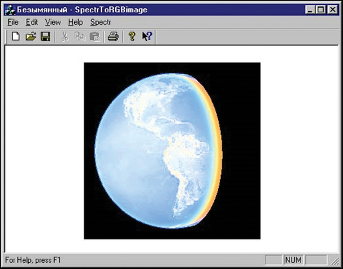
In order to model colour images of the Earth observed from different altitudes, we used the calculation results of Earth’s outgoing radiation according to the method described in Khokhlov (2001a). This method allows us to identify the specifications of radiation distribution over the disk of the planet, including the terminator region and the transition between the Earth’s surface and the atmosphere. As the first step involves only the most general features of the global distribution, not a detailed description of its regional specifics, we did not take into account inhomogeneous nature of the albedo distribution in order to reduce the time for calculating colour images. The calculations were performed using a uniform distribution with albedo value of 0.3, which corresponds to the Earth’s global albedo. However, even under these conditions, it took a PC with a clock frequency of 1 GHz about 12 hours to calculate a colour image of the Earth with a radius of 60 pixels (1 pixel corresponded to the Earth’s surface area of ~106 × 106 km²). The visualization results of the calculated data for eight colour spaces from Table 1 are presented in Figure 3. The images were calculated under the same conditions. The observation altitude was 376,000 km, and the nadir direction corresponded to a point on the Earth’s surface with coordinates 45°N and 30°E. The observation time was 21:00 UT, 20 March 2000.

Figure 3. Colour images of the Earth in various colour spaces with and without allowance for radiation brightness (upper and lower groups of images, respectively).

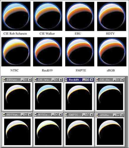
It can clearly be seen that allowance for radiation brightness adds less intensively illuminated regions to the image, as a result expanding it compared to the images that do not take brightness into account. It is also clearly visible how the use of different colour spaces affects the colour of the images. The most similarity is observed between the images in the CIE colour system.

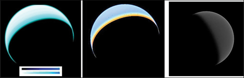
Hence, the CIE colour system with a higher spatial resolution of 32 × 32 km and no allowance for image brightness (see Table 1) was used for calculating Earth images. The results are presented in Figure 4. The images represent the view of the Earth at 21:00 UT; the date and the observation conditions are the same as in Figure 3. The left image demonstrates a visualization for a wavelength of 550 nm according to the method from (Khokhlov 2001b), the middle one – a visualization of the Earth’s radiation in the visible range (380–780 nm). The image on the left contains a calculated optical wedge, where the left side of the upper part corresponds to the minimum brightness, and the right side of the lower part – to the maximum brightness. For comparison, the same figure on the right shows an image of the Earth from (John 1996). The image is a 4° view of the Earth from the altitude of 240,000 km above the equator at 0° longitude, with the Sun overhead at 23°N and 110°E. This corresponds to a late evening (BST) around mid-summer in the Northern Hemisphere. The image only shows the light scattered by the atmosphere. The effect of the Earth’s shadow is clearly visible – the light reaches parts of the atmosphere above the surface points in the darkness. Unfortunately, the data set of the observation conditions is not complete, the image is grey and full comparison is not possible.

Figure 4. Calculated colour images of the Earth (Khokhlov 2001b) and an image from John (1996).

The simplified method allows us to construct images of the Earth observed from different altitudes. Figure 5 demonstrates some of the calculated images. Each image has a size of 101 × 101 pixels, and it takes about 12–15 minutes to calculate one on a medium-powered PC. The first group (a) contains images of the Earth at 500 nm, calculated from different altitudes at a 94° zenith angle of the Sun. The second group (b) presents images of the Earth from an altitude of 36,000 km for wavelengths of 800 and 2200 nm. A thin streak of dark Earth is visible in some images.

Figure 5. Calculated images of the Earth at wavelength of 500 nm from different altitudes (a) and different wavelengths (b).

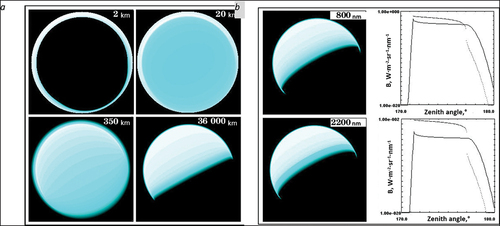
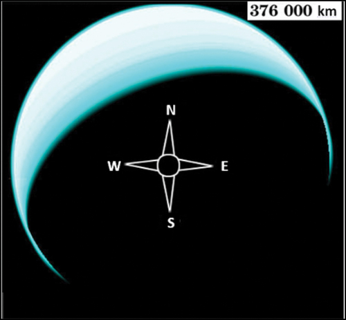
Figure 6 shows a 201 × 201 pixel image of the Earth from the near-lunar distance for the latitude of 40° and local midnight time. The atmosphere is clearly visible, especially its ‘whiskers’ over the dark Earth.

Figure 6. Image of the Earth from the near-lunar orbit.

At this stage, we used the colour representation of brightness on a logarithmic scale to visualize the calculation results.

2.4.2. The model of inhomogeneous distribution of the Earth’s surface albedo

To design the colour images of the Earth, observed from geostationary orbits, we used the calculated values of the Earth outgoing radiation according to the model described in detail in (Khokhlov (2001b).

We consider a spectrally indifferent, diffusely reflecting, but spatially inhomogeneous Earth’s surface, which we describe in terms of integral albedo global distribution, not a spectral one. We use a reference model of integral albedo global distribution, presented in Figure 2 with a resolution of 0.4° х 0.4°. This map is worked out based on physical maps and integral albedo data for various types of the Earth surface (Tverskoy 1962), presented in Table 2. To space the albedo values indicated in Table 1 over the surface we use the Earth physical map. Thus, for each point of the global surface, specified by geographic coordinates, we have the corresponding albedo value. For the result visual reference, we provide a map picture (Figure 2), not in black and white (256 gradations), but in pseudo colour (768 gradations). This map does not contain any information on the Earth surface colours.

Table 2. Albedo values for different types of surfaces (Tverskoy 1962).

Surface type	Albedo	Surface type	Albedo
Sea	0.04–0.18	Sand grey	0.18–0.23
Fallow (humid)	0.05–0.07	Meadow	0.19
Black soil (humid)	0.08	Corn, wheat in different ripening phases	0.10–0.25
Fallow (dry)	0.08–0.12	Blue clay (dry)	0.23
Grey earth (humid)	0.10–0.12	Granite	0.24
Pine-wood	0.12	Grass (fresh, dry)	0.26
Black soil (dry)	0.14	Grey earth (dry)	0.25–0.30
Forest cover	0.10–0.18	Snow (humid, dirty)	0.20–0.30
Ploughed field	0.14–0.17	Sand yellow	0.35
Basalt	0.14	Sea ice	0.30–0.40
Greenwood	0.15	River sand	0.35
Tundra	0.15–0.20	Clouds	0.46–0.73
Grey clay (humid)	0.16	Chalkstone	0.56
Grass (dried by sunlight)	0.19	Snow (fresh-fallen)	0.90

To convert albedo А values to RGB colours, they used parameter 0.3, which corresponds to the albedo value as

(13) $\mathrm{\Sigma }=73.93+693.79\cdot sin(\frac{\pi }{2}\cdot A)$(13)

Parameter ∑ value was converted into RGB colours according to the following rule:

(14) $\begin{array}{rl}& (0,0,\mathrm{\Sigma })0\le \mathrm{\Sigma }\le 255\\ & (0,\mathrm{\Sigma },255)255<\mathrm{\Sigma }\le 511\\ & (\mathrm{\Sigma },255,255)\hspace{0.17em}511<\mathrm{\Sigma }\le 767\end{array}$(14)

The map of the global albedo distribution shown in Figure 2 was converted into a binary file, which was further used for automatic albedo value calculation using geographic coordinates.

3. Results and discussion

1. Colour rendering of Earth images based on the model of radiation brightness of the spherical Earth’s atmosphere, taking into account inhomogeneous temperature and surface characteristics

The model is literal and involves three-dimensionally inhomogeneous distribution of atmospheric density in a spherical atmosphere and not only direct solar radiation but also a surface reflected one. The remarkable thing is that the model enables us to calculate the atmosphere brightness without any restrictions of directions, heights and observation time. As the input parameters it uses only the spectral region data, place, direction and Julian date (combining calendar date and time) of observation. This molecular scattering model in association with the experimental data, the assumed substantiation, application areas and limitations are discussed in Khokhlov (2001a, 2001b). The described model enables us to reveal the features of the radiation distribution transformation over the planetary molecular atmosphere, including the terminator area and the ‘Earth-atmosphere’ transfer. A typical example of the Earth image calculation with inhomogeneous surface temperature and albedo distribution is shown in Figure 7 in real colours, as it is perceived by human eyes.

Figure 7. The Earth calculated image, from the altitude of 36,000 km above the equator, 75 ° West longitude. Date: 27.09.2000 Time: 21 UT.

In Figure 8, the experimental images are shown for comparison. The calculated images in real colours (top row) are shown together with black and white images from the geostationary satellites METEOSAT, GMS, GOES-W and GOES-E (The Satellite Data Services (SDS) group 2020) (bottom row).

Figure 8. The Earth calculated and experimental images obtained from the geostationary orbits.

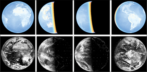
The calculated images were elaborated for the same conditions as the experimental ones. With that, only the place and time of observation were considered. The observation altitude is 36,000 km, the nadir direction corresponds to the equatorial points of the Earth’s surface with the longitudes indicated in Table 3 for each satellite. The date of satellite passage is 06.03.2006. The observation time is also indicated in Table 3.

Table 3. Observation conditions for geostationary satellites.

Satellite	Longitude, deg.	Time, UT
METEOSAT	0	12:00
GMS	140 E	09:00
GOES-W	135 W	03:30
GOES-E	75 W	15:00

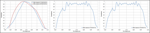
The calculations of colour theoretical images were performed with an allowance for instrumental spectral characteristics of all satellites. Figure 9 shows spectral characteristics for geostationary satellites of the early 20th century generation. These characteristics, covering the visible range, allow us to convert black-and-white images into colour ones; however, they either do not provide a set of input data required for calculations (David Woods and O’Brien 1968), including geostationarity of the orbit, or are published in black-and-white, sacrificing chromaticity in order to increase image resolution in the visible range. In the studies of natural phenomena, pseudo-colour images are typically used in the ultraviolet, near-, mid- and far-infrared ranges, as well as in the thermal range. Numerous visual colour images from low-flying satellites or satellites in polar orbits, such as Landsat, NOAA, Spot, Terra and other regional-scale systems, are available but not considered in this article.

Figure 9. Spectral characteristics of colour filters for geostationary satellites Meteosat (Filter Profile Service et al. 2012), GMS (Filter Profile Service et al. 2012a) and GEOS (Filter Profile Service et al. 2012b) of the early 20th century generation.

It is possible to compare the images only with black and white ones since most of the available colour images are artistic and pseudo-colour or do not contain full information on the calendar date, time, place and orientation of the observation direction.

The calculated and experimental image comparison shows close matching in general Earth’s brightness distribution, the continents outlines and random brightness distribution over the surface. Since cloudiness is not considered in the calculations, it is missed. The calculated images clearly reflect orange-red colours in the terminator area, related to glow phenomena. The blue colour of the calculated images is associated with solar radiation scattered by molecular constituents of the atmosphere. The most intense colours are over the oceans, where the contribution of the Earth’s surface radiation is less due to the small ocean waters’ albedo.

Comparison of colour and black-and-white images can be carried out only by the location of the Earth’s disk, phase and regional landscape of its surface. These characteristics are visually similar for all four satellites.

3.2. Comparison of theoretical and satellite colour images in the visible spectrum

To begin a discussion on the possibility of comparing the realistic colour rendering of theoretical models of the global state of the Earth’s atmosphere with satellite images of the Earth view from geostationary altitudes, let us consider the images in Figure 10.

Figure 10. Comparison of the calculated image for the GMS satellite (Himawari-5) and the image from the Himawari 8 satellite.

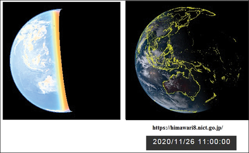
It is interesting to compare the theoretical image from the GMS satellite (Himawari-5) dated 2006/03/06 and the image from the modern Himawari 8 satellite (The Himawari-8 Real-time Web 2021) dated 2020/11/26. Figure 10 clearly shows the geometric and seasonal differences, explained by the interval of more than 14 years between the images.

At present, a number of satellites regularly take photographs of the full disk of the Earth. Three satellites, colour images of which are borrowed from West (2017) and shown in Figure 11, attract special attention. The first two satellites (Himawari-8 and GOES-16) are geostationary satellites that take images from an altitude of 35,785 km above the Earth’s equator. The third one, DSCOVR (Deep Space Climate Observatory), is located in the orbit between the Earth and the Sun, at a distance of about 1,500,000 km from the Earth at the Lagrange point L₁.

Figure 11. Colour images of the disk of the Earth, fully illuminated by the Sun (The SVO Filter Profile Service 2020).

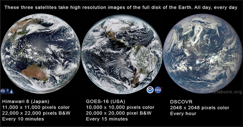
The geostationary satellite images in Figure 11 have high colour resolution and even greater resolution in black-and-white. The Earth Polychromatic Imaging Camera (EPIC) DSCOVR operates in low-resolution colour (EPIC is a 10-channel spectroradiometer (317–780 nm) onboard the NOAA’s DSCOVR spacecraft).

Spectral characteristics or quantum efficiency of the matrices for all three satellites are presented in Figure 12.

Figure 12. Spectral characteristics of colour filters for geostationary satellites Himawari (The SVO Filter Profile Service 2020),(Himawari-9 2018), GOES (Advanced Baseline Imager (ABI) 2017) and DSCOVR EPIC (EPIC (Earth Polychromatic Imaging Camera) 2018).

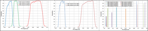
Images from Natural Color Imagery (2016) were created using 10 narrow spectral bands from EPIC that are within the visual range. They have colour and brightness adjusted to represent what a conventional camera would produce.

Unfortunately, due to the remoteness of the Earth and incomplete information about the parameters of the mandatory set of input data, the calculation using the model of outgoing Earth radiation for the DSCOVR satellite is currently impossible. For the same reason, the set of input data for calculating images of geostationary satellites has not been formed either.

4. Conclusions

This article addresses the possibility of colour rendering for the images of luminous planetary objects with gas and dust envelopes. Presented results of performed calculations indicate that there is a significant dependence between the colour palette of the image and the colour system used to convert the calculated data into images. Nevertheless, almost all colour systems can realistically represent the distribution of colour depending on illumination of the Earth by the Sun.

A specific aspect of the proposed method for calculating colour images of the Earth is the use of a spherical model based on physical principles. The model is limited by the choice of Rayleigh scattering processes of solar radiation coming from the Earth’s atmosphere. The model takes into account the following processes:

• Single scattering of direct solar radiation in the atmosphere;

• Reflection of solar radiation from the inhomogeneous Earth’s surface, transmitted and dispersed into space by the atmosphere.

A characteristic feature of the model is the representation of inhomogeneous distribution of the Earth’s surface albedo, surface temperature and altitude profile of the density of the main gas components.

The calculated values, presented in this article with an allowance for instrumental spectral distributions, demonstrate a realistic picture of colour brightness distribution of the Earth image depending on its illumination by the Sun. The planet appears light blue in the brightly illuminated part of the Earth’s disk and orange-red in the luminous segment of the terminator.

The authors indicate the difficulties associated with comparing theoretical and experimental images of the full disk of the Earth in the visible range in natural colours. The reasons behind those include the incompleteness of information about the observation conditions of satellite colour images and the preference for obtaining the results in black-and-white due to the fourfold increase in the resolution of Earth images. This is especially true for high-altitude satellites and spacecraft.

One application of the material in this article is the use of the Moon’s ash light emission as a tool for studying the Earth’s global albedo. Measurements of the Moon’s ash light are a challenging task currently being undertaken by astronomers in the United States (Big Bear Lake Solar Observatory in California), Russia (Novolazarevskaya Station in Antarctica) and several other countries in the deployment phase.

To control the experimental data in our research on this subject, we use the results of theoretical calculations of images of the Earth as it is seen from the Moon and from a height of 36,000 km above the Novolazarevskaya station. For the same purpose, the experimental and theoretical images of the Moon at the time of the experiment are compared.

Acknowledgements

This research has made use of the SVO Filter Profile Service (http://svo2.cab.inta-csic.es/theory/fps/) supported by the Spanish MINECO through grant AYA2017-84089.

The research was performed at the expense of the subsidy for the state assignment in the field of scientific activity for 2021 #FSRWW-2020-0014.

The authors would like to thank anonymous reviewers for their constructive comments on an earlier version of this paper.

Disclosure statement

No potential conflict of interest was reported by the author(s).

Correction Statement

This article has been corrected with minor changes. These changes do not impact the academic content of the article.

Appendix A

A brief history

A1. The history of computer graphics

• Industrial and military production. The beginning of the space era was preceded by successful developments of John T. Parsons (Parsons 1958) in the field of computer-controlled machines for industrial and military production, which started in 1950s. The new technology was called computer numerical control (CNC). The time-consuming process of developing and debugging CNC punched tape programs was soon fully automated using Whirlwind and TX-0 computers. This automation technology was named APT (Automatically Programmed Tool) and factually became the predecessor of modern CAD (Computer Aided Design) software (Douglas 1959).

Parsons was engaged in the design and development of unique manufacturing processes and equipment for the US Air Force (R-5 Sikorsky helicopter and Ercoupe aircraft), installation of equipment for the production of the Minuteman rocket and the Saturn launch vehicle. In 1963, a complete facility was designed for the production of monobloc ship propellers for the US Navy; in 1971 – the N/C system for the automatic inspection of turbine blades. Since 1973, John T. Parsons initiated design studies on rotor blades for large wind energy systems.

• Computerization of technologies. In the middle of the 20^th century, development of communication technologies contributed to the rapid transition from mechanical calculators, the first prototype of which was described by Leonardo da Vinci in 1492 (Rafael 2013), to electronic computers. Michael Noll (Michael Noll 1967), a pioneer in the area of computer-generated 3D movies at Bell Telephone Laboratories in the 1960s, explained the role of a computer as a powerful tool that can perform quick computation and manipulation of large number arrays but is incapable of true creativity.

It can be considered that the era of computer graphics began in December 1951, when researchers at the Massachusetts Institute of Technology (MIT) developed the first display for the ‘Whirlwind’ computer at the request of the air defence system of the US Navy. The inventor of this display was an MIT engineer Jay Forrester.

The first officially recognized attempt to use a display to obtain an image output from the computer was the invention of the Whirlwind-I machine at MIT in 1950. Subsequently, Whirlwind became the prototype for a whole range of computers, which allowed to develop an extensive US air defence system – SAGE (Semiautomatic Ground Environment) (WHIRLWIND 1953). From 1952 and until the deployment of the SAGE system, Jay Forrester was in charge of its development.

In the scope of the SAGE programme, a unique basis for further development of computer graphics was created with the development of computer networks and their long-term coexistence with CNC and CAD. However, almost all companies still used the classic paper-based carriers (tapes and punched tapes) for transferring data to machine tools. The situation changed drastically after 1963, when Ivan Sutherland (one of the founding fathers of computer graphics) developed a hardware-software complex Sketchpad (Sutherland 2003) as part of his doctoral dissertation.

What is unique about Sketchpad is that it had defined a graphical user interface more than 20 years before the term was actually used for the first time. The Sketchpad system utilized sketches as a new communication tool between the user and the computer. The Sketchpad system contained input, output and computation programs, which allowed it to interpret information directly from the computer display. However, even current multidisciplinary scientific computer graphics (CG) do not allow for computational experiments with high-resolution visualization of the results.

It became a general-purpose system for the TX-2 computer (allowed to make sketches of electrical, mechanical, scientific, mathematical images and animated drawings), with software written in the ‘macroassembler’ language.

Technology of art and the dawn of computer graphics. Following the success of the first experiments in the industrial, military and computer fields, a Boeing research programme with William A. Fetter as its leader was launched in November 1960. The result of research was registered as a US patent ‘Planar Illustration Method and Apparatus’ (Walter 1969, Barnet 1965). The article (Barnet 1965) deals with the role of art and technology in the development of computer graphics. As an artist, Fetter described the process by perspective drawing on the chalkboard and then allowed others to develop a software program with mathematically equivalent operations. In his lectures, Fetter demonstrated a movie ‘SST Cockpit Visibility simulation’ in 1966. The first human figure, which he managed with a computer for a film, however, was the Landing Signal Officer on a CV-A 59 aircraft carrier. The figure was shown in a short CV A-59 film but only as a silhouette and not as detailed elaboration as the First Man had been. Fetter published this in November 1964 in his book Computer Graphics in Communication in the section ‘Aircraft Carrier Landing Depiction with images’ (William 1965).

The term ‘computer graphics’ was first used in 1960 at the Wichita branch of the Military Aircraft Systems Division of Boeing. It was coined by William Fetter and his superior Verne Hudson (Oppenheimer 2005, Jump 1966). The first actual application of computer graphics is associated with the name of John Whitney, a filmmaker in the 1950–60s, who was the first to use a computer of his own invention to create animated title sequences. A demonstration reel by J. Whitney, created with his analogue computer/film camera magic machine, which he built from a World War II anti-aircraft gun sight (Whitney 1961), as well as three-dimensional computer images by W. Fetter were displayed at the exhibition ‘Cybernetic Serendipity: Computer and Art’ at the London Institute of Contemporary Arts, which in 1968 was curated by J. Reichardt. It was one of the pivotal exhibitions of computer art and digital installations in the late 1960s and the early 1970s, attended by such important figures in the world of technological art of that time, as Charles Csuri, Michael Noll, Nam June Paik, Frieder Nake, John Whitney, John Cage, etc.

A2 Computer graphics and its applications

The development of computer graphics (CG) followed the evolution of computers and software. CNC and APT technologies, tested under military contracts (predecessors of modern CAD technologies), the Sketchpad complex, the Whirlwind computer, projects of art and digital installations, developed by long-term efforts of researchers, designers, engineers, as well as artists, inventors, software engineers and IT specialists, have become indispensable necessities in the life of the global community.

The very first CG applications took place in the fields of scientific research, computer video games and video films (William 1965). The first bulky prototypes of computers were used only for solving scientific and industrial problems. Modern diversified scientific CG makes it possible to perform computational experiments and to provide the visual representation of their results.

Nowadays, the most productive and well-known CG applications are associated with film and entertainment industries, where image synthesis is used to create visually appealing special effects for movies and video games. CG transforms the results of solved problems into visual representations of various information; it is widely used in all branches of science, technology, medicine, commercial and management activities. Being an indispensable element of CAD software, CG prevails in the work of design engineers, architects and inventors of new equipment. Design, construction and detailed drafting of workpieces are carried out using CG tools, which allow to obtain both flat and 3D images. Due to television and Internet, CG has also found its application in such spheres as art, illustration, animation and advertising.

References

- Advanced Baseline Imager (ABI). 2017. “PFM, on Board GOES-16.” http://svo2.cab.inta-csic.es/theory/fps/index.php?mode=browse&gname=GOES&asttype=earth
- Barnett, J. 1965. “Will the Computer Change the Practice of Architecture?” In Architectural Record 1 , Vol. 137 (Detroit: BNP Media). January. 149.
- Berk, A., L. Bernstein, and D. C. Robertson MODTRAN. “A Moderate Resolution Model for LOWTRAN.” 1987, https://www.researchgate.net/publication/235184147_MODTRAN_A_moderate_resolution_model_for_LOWTRAN
- Berk, A., P. Conforti, R. Kennett, T. Perkins, F. Hawes, and J. Bosch. 13 June 2014. “MODTRAN6: A Major Upgrade of the MODTRAN Radiative Transfer code, Proc.” Spie 9088, Algorithms and Technologies for Multispectral, Hyperspectral, and Ultraspectral Imagery XX, 90880H & 9088, Algorithms and Technologies for Multispectral, Hyperspectral, and Ultraspectral Imagery XX, 90880H 10.1117/12.2050433.
- Chepyzhova, A. V., E. A. Pravdina, and O. Y. Lepikhina. “Comparative Evaluation of the Effectiveness of the Laser Scanning and Aerial Photography Systems Using Unmanned Aerial Vehicles.” Journal of Physics: Conference Series Novosibirsk, Russia 2019, 1333. doi:10.1088/1742-6596/1333/3/032064. ( 3).
- CIE Proceedings. 1964. Vienna Session. 1963 Vols. B, P. 209–220. Committee Report E-1.4.1 Paris: Bureau Central de la CIE.
- David Woods, W., and F. O’Brien. 1968. “Apollo 8 Day 1: The Green Team and Separation.” https://history.nasa.gov/afj/ap08fj/03day1_green_sep.html
- Douglas, R. T. 1959. Servomechanisms Laboratory Department of Electrical Engineering Massachusetts Institute of Technology, 86. United States: Department of Electrical Engineering Massachusetts Institute of Technology. http://www.bitsavers.org/pdf/mit/whirlwind/apt/APT_System_Volume_1_General_Description_of_the_APT_System_1959.pdf
- EPIC (Earth Polychromatic Imaging Camera). 2018. “Is a 10-channel Spectroradiometer (317 – 780 Nm) Onboard NOAA’s DSCOVR (Deep Space Climate Observatory) Spacecraft.” http://svo2.cab.inta-csic.es/svo/theory/fps3/index.php?mode=browse&gname=DSCOVR&asttype
- Fairchild, M. D. 2013. “Color Appearance Models.” In Wiley-IS&T Series in Imaging Science and Technology, 3, P. 472. Hoboken: John Wiley & Sons. 9781. 9781119967033119967033
- Filter Profile Service, T. S. V. O., C. Rodrigo, E. Solano, and A. Bayo, 2012 http://svo2.cab.inta-csic.es/theory/fps/index.php?mode=browse&gname=Meteosat&asttype=earth
- Filter Profile Service, T. S. V. O., C. Rodrigo, E. Solano, and A. Bayo, 2012a http://svo2.cab.inta-csic.es/theory/fps/index.php?mode=browse&gname=Himawari&gname2=GMS5&asttype=earth
- Filter Profile Service, T. S. V. O., C. Rodrigo, E. Solano, and A. Bayo, 2012b http://svo2.cab.inta-csic.es/theory/fps/index.php?mode=browse&gname=GOES&gname2=Imager11&asttype=earth
- Ford, A., and A. Roberts. “Colour Space Conversions.” 11 August 1998 https://studylib.net/doc/18082326/colour-space-conversions
- Guild, J. 1931. “The Colorimetric Properties of the Spectrum.” Philosophical Transactions of the Royal Society 230: 149–187. doi:10.1098/RSPB.1931.0091.
- Guo, H., J. Cao, H. Wang, J. Zhang, and H. Yang. 2014. “Color Management of sRGB Color Space for HDR Digital Camera.” Hongwai Yu Jiguang Gongcheng/Infrared and Laser Engineering 43: 238–242.
- The Himawari-8 Real-time Web 2021 https://himavari8.nict.go.jp/
- Himawari-9. 2018. “Advanced Himawari Imager (AHI-9) Instrument.” http://svo2.cab.inta-csic.es/theory/fps/index.php?id=Himawari/AHI9.Band01&&mode=browse&asttype=earth&gname=Himawari&gname2=AHI9#filter
- HosseiniHaghighi, S., F. Izadi, R. Padsala, and U. Eicker. 2020. “Using Climate-Sensitive 3D City Modeling to Analyze Outdoor Thermal Comfort in Urban Areas.” International Journal of Geo-Information 9 688.
- Ignatiev, S. A., and D. S. Kessel. 2016. “Effect of Surface Geometry and Insolation on Temperature Profile of Green Roof in Saint-Petersburg Environment.” Journal of Mining Institute 220: 622–626.
- John, I. 1996. Full-Spectral Rendering of the Earth’s Atmosphere Using a Physical Model of Rayleigh Scattering (March, 1996) Computer Graphics Unit. Manchester: Manchester Computing, University of Manchester. M13 9PL http://citeseerx.ist.psu.edu/viewdoc/download;jsessionid=55743436B4E3634187CBBF8FA52B903C?doi=10.1.1.49.7170&rep=rep1&type=pdf
- Jump up to: a b William Fetter: Computer Graphics at Boeing. “Print Magazine.” XX:VI, November 1966, S. 32
- Kaneda, K., T. Okamoto, E. Nakamae, and T. Nishita. 1991. “Photorealistic Image Synthesis for Outdoor Scenery under Various Atmospheric conditions.“ The Visual Computer 7 (5–6): 247–258. doi:10.1007/BF01905690.
- Kazantsev, A., A. Boikov, and V. Valkov. “Monitoring the Deformation of the Earth’s Surface in the Zone of Influence Construction.” (2020) E3S Web of Conferences October 24-26, 2019 Khabarovsk, Russia, 157, DOI: 10.1051/e3sconf/202015702013.
- Khokhlov, V. N. 2001a. “Rayleigh Scattering in the Atmospheres of the Planets, Taking into Account the Inhomogeneous Temperature Distribution and Albedo of Their Surfaces.” Journal of Optical Technology 68 (2): 23–32.
- Khokhlov, V. N. 2001b. “Results of Modeling Rayleigh Scattering in the Earth’s Atmosphere with an Inhomogeneous Albedo and Temperature Distribution on Its Surface.” Journal of Optical Technology 68 (2): 105–109. doi:10.1364/JOT.68.000105.
- Khokhlov, V. N., L. A. Mirzoeva, N. N. Naumova, and O. O. Obvintzeva. “Comparison of Remote Sensing Technologies of Global the Earth’s Climate Changes.” Conference Proceedings: The 31st International Symposium on Remote Sensing of Environment (IRSE - 2005) St. Petersburg, Russia, IRSE, 2005. 4
- Klassen, R. 1987. “Modeling the Effect of the Atmosphere on light. ACM Trans.” Graph 6: 215–237. doi:10.1145/35068.35071.
- Kneizys, F. X., L. W. A. Eric Shettle, and J. H. Chetwynd. “User Guide to LOWTRAN 7.” August 1988, https://www.researchgate.net/publication/235203858_User_guide_to_LOWTRAN_7
- Kneizys, F. X., E. Shettle, W. Gallery, and L. W. A. Chetwynd J. H Jr. 1983. Atmospheric Transmittance/Radiance: Computer Code LOWTRAN 6. Atmospheric_TransmittanceRadiance_Computer_Code_LO.pdf. August, Supplement: Program Listings.
- Kopylova, N. S., and I. P. Starikov. “Fresh Approaches to Earth Surface Modeling.” (2018) Journal of Physics: Conference Series, 1015 (3), DOI: 10.1088/1742-6596/1015/3/032062.
- Koteleva, N., and I. Frenkel. 2021. “Digital Processing of Seismic Data from Open-Pit Mining Blasts.” Applied Sciences 11 (1): 383. doi:10.3390/app11010383.
- Kovyazin, V. F., P. M. Demidova, D. T. Lan Anh, D. V. Hung, and N. Van Quyet. 2020a. “Monitoring of Forest Land Cover Change in Binh Chau - Phuoc Buu Nature Reserve in Vietnam Using Remote Sensing Methods and GIS Techniques.” IOP Conference Series: Earth and Environmental Science 507 (1). doi:10.1088/1755-1315/507/1/012014.
- Kovyazin, V. F., A. Y. Romanchikov, D. T. Lan Anh, D. V. Hung, D. T. Lan Anh, and D. V. Hung. 2020b. “Monitoring of Forest Land Use/Cover Change in Cat Tien National Park, Dong Nai Province, Vietnam Using Remote Sensing and GIS Techniques.” IOP Conference Series: Materials Science and Engineering 817 (1): 012018. doi:10.1088/1757-899X/817/1/012018.
- Kozhaev, Z. T., M. A. Mukhamedgalieva, M. G. Mustafin, and B. B. Imansakipova. 2017. “Geoinformation System for Geomechanical Monitoring of Ore Deposits Using Spaceborn Radar Interferometry Methods.” Gornyi Zhurnal 2: 39–44. doi:10.17580/gzh.2017.02.07.
- Littlefair. 1994. “Paul A Comparison of Sky Luminance Models with Measured Data from Garston.” United Kingdom. Solar Energy 53 (4): 315–322. doi:10.1016/0038-092X(94)90034-5.
- Longtin, D. R., N. L. DePiero, F. M. Pagliughi, and J. Hummel. “SENTRAN7: The Sensitivity Package for LOWTRAN7 and MODTRAN.” Volume 2 November 1991, https://www.researchgate.net/publication/235168108_SENTRAN7_The_Sensitivity_Package_for_LOWTRAN7_and_MODTRAN_Volume_2
- Longtin, D. R., and J. Hummel. “Users Guide for SENTRAN7, Version 2.0.” August 1993, https://www.researchgate.net/publication/235082841_Users_Guide_for_SENTRAN7_Version_2
- Makhov, V. E., and I. I. Sytko. 2018. “Shape and Relief Evaluation Using the Light Field Camera.” IOP Conference Series: Earth and Environmental Science 194 (2). doi:10.1088/1755-1315/194/2/022020.
- Michael Noll, A. 1967. “The Digital Computer as a Creative Medium.” IEEE Spectrum 4 (10, October): 89–95. doi:10.1109/MSPEC.1967.5217127.
- Musta, L. G., G. N. Zhurov, and V. V. Belyaev. “Modeling of a Solar Radiation Flow on an Inclined Arbitrarily Oriented Surface.” (2019) Journal of Physics: Conference Series, 1333 (3), DOI: 10.1088/1742-6596/1333/3/032054.
- Natural Color Imagery 2016 https://epic.gsfc.nasa.gov/about
- Nishita, T., and Y. Dobashi. “Modeling and Rendering of Various Natural Phenomena Consisting of Particles.” Proceedings. Computer Graphics International 2001, Hong Kong, China, 2001; pp. 149–156, DOI: 10.1109/CGI.2001.934669.
- Nishita, T., Y. Dobashi, K. Kaneda, and H. Yamashita. 1996. “Display Method of the Sky Color Taking into Account Multiple Scattering.” In Pacific Graphics Vol. 96, P. 117–132. Taiwan: Department of Computer Science, National Tsing Hua University.
- Oppenheimer, R., and E. A. T. William Fetter, and 1960s. “Computer Graphics Collaborations in Seattle.” www.academia.edu,https://www.historylink.org/File/20542
- Parsons, J.T.and F.L. Stulen. Patented 14 January1958. “Motor controlled apparatus for positioning machine tool.“ https://patentimages.storage.googleapis.com/11/89/bc/16daaf50a6a9e0/US2820187.pdf
- Preetham, A. J., P. Shirley, and B. E. Smits. “A Practical Analytical Model for Daylight.” Proceedings of the 26th annual conference on Computer graphics and interactive techniques Los Angeles, CA, United States (NY, United States: ACM Press/Addison-Wesley Publishing Co.) 1999, P. 91–100, DOI: 10.1145/311535.311545.
- Project WHIRLWIND summery report №. 35 third quarter. 1953. “Digital Computer Laboratory Massachusetts Institute of Technology.” http://www.bitsavers.org/pdf/mit/whirlwind/Project_Whirlwind_Summary_Report_No_35_Third_Quarter_1953.pdf
- Rafael, Fraguas. 2013. “El País. Madrid“ edited by Código Da Vinci a la castellana.
- Rodionov, V. A., S. A. Tursenev, I. L. Skripnik, and Y. G. Ksenofontov. 2020. “Results of the Study of Kinetic Parameters of Spontaneous Combustion of Coal Dust.” Journal of Mining Institute 246: 617–622. doi:10.31897/PMI.2020.6.3.
- Rothman, L. S., I. E. Gordon, Y. Babikov, A. Barbe, D. C. Benner, P. F. Bernath, M. Birk, et al. 2013. “The HITRAN2012 Molecular Spectroscopic Database.” Journal of Quantitative Spectroscopy and Radiative Transfer 130 (November): 4–50.
- The Satellite Data Services (SDS) group. “University of Wisconsin-Madison.” 2020, https://inventory.ssec.wisc.edu/inventory/
- Selby, J. E. A., and R. A. McClatchey. 1975. Atmospheric Transmittance from 0.25 to 28.5 um: Computer Code LOWTRAN 3,109. United States: Optical Physics Laboratory, Air Force Cambridge Research Laboratories.
- Shutterstock. Available online: https://www.shutterstock.com (accessed on 26 November 2020)
- Smith, T., and J. Guild. 1931–32. “The C.I.E. Colorimetric Standards and Their Use.” Transactions of the Optical Society 33 (3): 73–134. doi:10.1088/1475-4878/33/3/301.
- Speranskaya, N. I. 1959. “Determination of Spectrum Color Coordinates for Twenty-seven Normal Observers.” Optics and Spectroscopy 7: 424–428.
- Stiles, W. S., and J. M. Burch. 1959. “NPL Colour-matching Investigation: Final Report.” Optica Acta: International Journal of Optics 6 (1): 1–26. doi:10.1080/713826267.
- Strizhenok, A. V., A. V. Ivanov, and I. K. Suprun. “Methods of Decoding of the Geoecological Conditions of natural-Anthropogenic Complexes Based on the Data of Earth Remote Sensing.” (2019) Journal of Physics: Conference Series, 1399 (4), DOI: 10.1088/1742-6596/1399/4/044077.
- Sutherland, I.E. . 2003. Sketchpad: A Man-machine Graphical Communication System, 149. United Kingdom: University of Cambridge. https://www.cl.cam.ac.uk/techreports/UCAM-CL-TR-574.pdf. doi: 10.48456/tr-574.
- The SVO Filter Profile Service. “Rodrigo C. Solano E.” 2020; https://ui.adsabs.harvard.edu/abs/2020sea.confE.182R/abstract
- Tomoyuki, N., S. Takao, T. Katsumi, and N. Eihachiro. “Display of the Earth Taking into Account Atmospheric Scattering.” In Proceedings of the 20th annual conference on Computer graphics and interactive techniques (SIGGRAPH ‘93). Association for Computing Machinery, New York, NY, USA, 1993; P.175–182.DOI: 10.1145/166117.166140.
- Tverskoy, P. N. 1962. Meteorology Course, 700. Russia: Publisher: L., Gidrometizdat.
- Walker, J. 2004. “Colour Rendering of Spectra.” https://www.fourmilab.ch/documents/specrend/
- Walter, D., Bernhart, and A. William. 1969. Fetter: US Patent.
- West, M. “Full-Disk HD Images of the Earth from Satellites.” 2017 https://www.metabunk.org/threads/full-disk-hd-images-of-the-earth-from-satellites.8676/
- Whitney, J. ”Catalog” 1961. https://www.youtube.com/watch?v=TbV7loKp69s
- William, A. F. 1965. Computer Graphics in Communication, 110. United States: McGraw-Hill.
- Wright, W. D. 1929. “A Redetermination of the Trichromatic Coefficients of the Spectral Colours.” Transactions of the Optical Society 30 (4): 141–164. doi:10.1088/1475-4878/30/4/301.
- Zotti, G. “Dissertation.” Computer Graphics in Historical and Modern Sky Observations. Wien, 29 October 2007 https://www.cg.tuwien.ac.at/research/publications/2007/zotti-2007-PhD/zotti-2007-PhD-pdf.pdf