Urban growth dynamics modeling through urban DNA in Tehran metropolitan region

ABSTRACT

The spatial models dealing with urban growth dynamics have been widely studied, while rare works have considered under-developed countries. Several problems have been detected in creating, calibrating and applying urban growth models and changing land use. The present work aims the modelling land-use changes through the CA-GA model in which a frame is provided for analysis and producing a map of growth patterns in urban areas in different spatial scales to study and analyse the increasing urban growth in Tehran. To consider the land-use changes in Tehran, ETM+TM images of 1985, 1992, 2000, and 2020 were selected to be analysed by the CA-GA algorithm to model the growth of the urban areas. The total kappa of results in Tehran is about 0.93, indicating the required precision and confidence of applied combinative genetic-Cellular automata modelling methods to model urban development.

KEYWORDS:

• Urban growth modelling
• Tehran metropolitan
• urban DNA
• cellular automata
• genetic algorithm

1. Introduction

The analysis of spatial configuration and urban growth dynamics is of a great deal of importance in contemporary urban studies, which have been studied by many researchers (Acioly and Davidson 1996; Wang et al. 2003; Páez and Scott 2004; Hedblom and Soderstrom 2008; Syphard, Clarke, and Franklin 2005; Geymen and Baz 2008; Robert 2013; Rienow and Goetzke 2014; Hosseini et al. 2015). The urban growth dynamics have substantial environmental and regional implications that require meticulous products (Grimm et al., 2008). The consequences of proper or improper urban growth are evaluated based on social and economic effects. By the way, the main consequences: increasing construction and public services costs (Brueckner 2000; Heimlich and Anderson 2001; Barnes et al. 2001; Wasserman 2000), waste of energy resources (Newman and Kenworthy 1988), inequality in wealth distribution (Mitchell 2001; Stoel 1999; Wilson et al. 2003), wildlife and ecosystem effects on (Grimm et al. 2000; Hedblom and Soderstrom 2008, waste of farms (Nelson and Moore 1993; Zhang 2003), temperature increase (Weng, Liu, and Lu 2007; Wang et al. 2007), impact on weather (Stone 2008; Stoel 1999; Frumkin 2002), impact on quality and quantity of water, (Jacquin, Misakova, and Gay 2008; Wasserman 2000), and health and social effects (Frumkin 2002; Savitch et al. 1993).

Thus, a precise assessment of urban growth and formal and informal process resulting in urban growth is required to ensure the permanent urban growth and diminishing the inappropriate environmental effects (Kanaroglou and Scott 2016), since each urban area undergoes a specific formation under exclusive urban DNA. Many studies have proven that a collection of factors, which comprehensively describes the urban growth process, has never been proposed regarding the fact that each case study has its own exclusive specificities (Dubovyk, 2010; Huang, Yeh, and Chang 2009; Cheng and Masser 2003; Hu and Lo 2007; Verburg et al. 2004).

In recent decades, the urban DNA has been studied by many researchers as a connector between urban models with similar evolution biology (Langton 1986; Openshaw and Openshaw 1997; Batty and Longley 1994; Batty and Xie 1996; Webster, 1996; Silva, 2001; Silva and Clarke 2002; Silva, 2004, 2005; Silva 2006). Similar to biological DNA, the main assumption of urban DNA is based on the fact that the main elements of a city determine its future growth. Thus, the geographic issues are evaluated based on geographic parameters (Rienow and Goetzke 2014).

Thus, the modelling of spatial processes is a powerful technique to understand the motives of urban landscape dynamics and evaluate the environmental and ecological effects. These models are of critical importance since they can model the dynamics of urban landscapes to support the regional and urban planning and permanent development (Wu and Martin 2002; Wu 2010). The urban growth modelling has been based on the CA models during recent decades (Xie and Batty 1996; Couclelis, 1997; Batty and Xie, 1997; Batty et al., 1999; Clarke et al., 1997; Clarke and Gaydos, 1998; White and Engelen 1997, 2000; Wu and Webster 1998; Yeh and Li 2000, 2001, 2002; Barredo et al., 2003; Wu et al., 2009; Heinsch et al., 2012; Rienow and Goetzke 2014).

The CA-based model is a dynamic model which uses the local interactions to simulate the evolution of system. Its main elements include lattice, cell state, neighbourhood and transition rules (White and Engelen 1997, 2000; Barredo et al., 2003). In this model, the mutual and nonlinear relations between subsystems are emphasized to understand the urban processes. In fact, the main property of urban CA models is to simulate the macrostructures based on mutual relations between local elements (Batty and Xie, 1997). The spatiotemporal complicacies of urban development are appropriately simulated by CA models (Wu and Webster 1998; Yeh and Li, 2002). Besides, a regional change pattern is currently formed of colliding local changes in a CA model where the evolution making simulation is often based on local interactions which means that this approach concentrates on small cells of the interactions between cells and spatial patterns are often neglected. Thus, the most critical point is how to consider the land converting behaviours in simplified cellular automata mechanisms in order to a better simulation of urban development (Wu and Webster 1998). Also, the neighbourhood rules are important and should be considered (O’Sullivan and Torrens 2000). Thus, the calibration techniques have been developed including the transition rules (such as slope, distance, etc), weight matrices, urban dynamics assessment models, multiple criteria decision-making analysis, CA-MAS model, logistic regression, CLUE-s, Markov chains, SLEUTH model, artificial intelligence and neural networks, Bayesian networks, Support Vector Machines, core learning-based methods, data mining and phase logics. The artificial intelligence methods are applied to solve the problems in which the parameter transition rules are not straightforward and they can be used to improve the automatic learning and optimize the parameters in order to modify and improve the precision and accuracy of CA simulation (Liu, Nishiyama, and Yano 2008; Liu and Yang 2008). A CA model can be developed with a combinative method. The genetic algorithm can be used to look for optimum result of problems based on the genetic mechanisms and evolution. The genetic algorithm has been inspired from genetics and Darwin’s evolution theory in which the survival of superiors or natural selection. The genetic algorithm is currently applied as an optimizing function. Also, it is a useful tool to understand the image and machine learning (Tseng and Yang 1997; Vafaie and Imam 1994).

In genetic algorithms, the evolution of organisms is simulated. They can be considered as oriented stochastic optimization, which tends to optimum point gradually. Compared to other optimization methods, this method can be applied to every problem without any knowledge about the problem and any constraints on the variables and hence a proven efficiency to find the general optimum. The main capability of this method is solving the complicated optimization problems in which classic methods are not applicable or not reliable to find the general optimum (Fogel 2000). Genetic algorithm has been widely used to solve the optimization problems related to geographic systems. In urban studies based on CA, the current combined method of Cellular automata with genetic algorithm has been proposed and applied in Cellular automata model to simulate the urban growth.

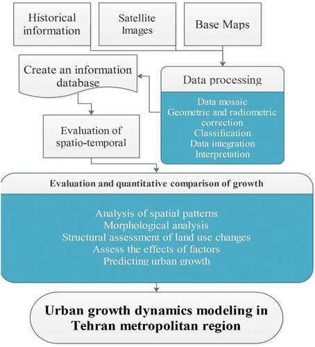
In this work, a self-consistent method is proposed to simulate the urban growth dynamics of metropolitan regions through simulating the parameters and CA transition rules. Here, the modelling frame includes the CA urban expansion which is related to an optimization factor through genetic algorithm to find the optimum basis set of transition rules and parameters. Finally, the optimum system of rules and parameters is proposed to assess the dynamics of urban expansion in Tehran metropolitan regions during 1985–2020 and forecasts the expansion pattern of urban regions regarding the exclusive DNA of this metropolitan (Figure 1).

Figure 1. Introduction Presentation of Research Structure.

The region of study

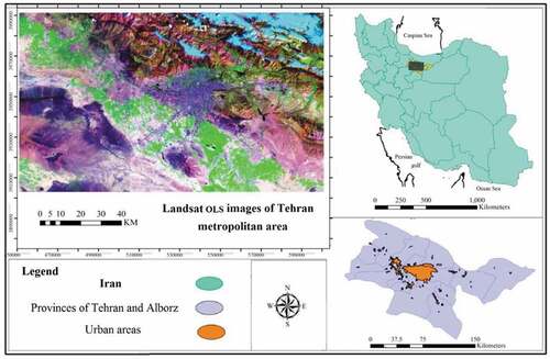
The region of the present work is the Tehran metropolitan including Tehran and Alborz provinces. The metropolitan region of Tehran is the urban or public region was named for the first time in 1994 based on a directive of council of ministers to present a framework of Tehran management relating to the suburban areas. In satellite images analysis, Firouzkooh town is not located in this area regarding large distance and negligible effect. Thus, this region exceeds 1,197,000 hectares, as shown in Figure 2 in the Iran map.

Figure 2. Tehran Urban Area on Iran land.

Methodology

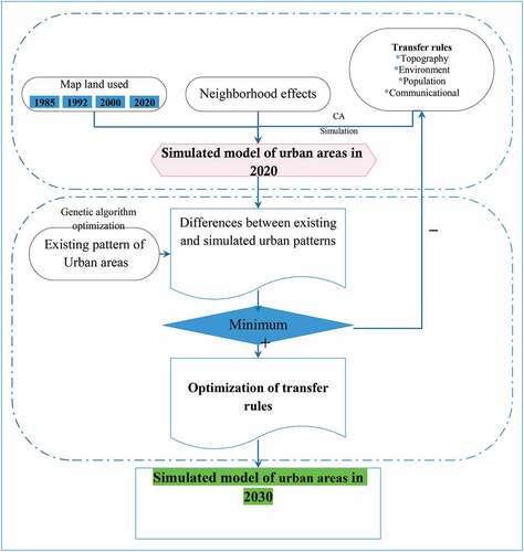
In this work, CA model is used to simulate urban growth to optimize the parameters and transition rules based on genetic algorithm model. The optimization process is done by minimizing the difference between observed urban coverage and its simulated surface. The model was applied to simulate the urban coverage variations in Tehran metropolitan area during 1985–2020. The CA models are often applied to simulate the spatiotemporal systematic processes and probable behaviour of changing the urban coverage. The urban model based on CA describes the transition rules or the change state of a cell during the time. CA models are based on perception and are able to combine both spatial and temporal dimensions of earth evolution in a simulation process. A CA model can be developed by a combinative method. The genetic algorithm can be used to find the optimum point for problems based on genetic mechanisms and natural selection. This algorithm has been applied to solve the optimization problems of many geographic systems. In CA-based urban studies, the current method formed of combination of CA and genetic algorithm has been used to simulate the urban growth. The present work is targeted to optimize the transition rules of urban coverage and CA parameters using genetic algorithm (Xiao et al. 2007; Santé et al. 2010). Here, the modelling framework includes the urban growth of CA which is related to an optimization unit using genetic algorithm to find the optimum system of transition rules and parameters. Then, the optimum obtained system is applied to simulate the dynamics of growth process. Each repeat in model indicates a year. A schematic modelling is shown in Figure 3.

Figure 3. Schematic Modelling.

The filter is integral to the action of the CAAutomata component. Its purpose is to down-weight the suitability of pixels that are distant from existing instances of the land cover type under consideration. The net effect is that to be a likely choice for land cover conversion, the pixel must be both inherently suitable and near to existing areas of that class. The default 5 × 5 filter (Moore neighbourhoods) has the following kernel: (00100,01110,1111 1, 01110, and 00100).

CA automatically normalizes the filter kernel to force the values to sum to 1 (thus the values ultimately vary from 0 to 0.0076). This filter is passed over a Boolean image for each class from the current land cover image within each iteration. Following this, a value of 0.1111 is added to the filtered results to produce a set of weight images. These are multiplied by the original suitability maps to down-weight suitability’s distant from existing areas of each class. The results are then stretched back to a byte (0–255) range. The net effect is that down-weighted suitability never exceed a down-weighting in excess of 90% of their original value. This ensures that suitable areas can be found if none are available in proximate areas.

Firstly, a system of rules and parameters of CA model is configured using logistic regression method.

Based on Bayes theorem, the probability of conversion of a cell to urban coverage at r and t+ Δt at t time is shown as follows:

$P\left(z\left(r,t+\mathrm{\Delta }t\right)=1|z\left(r,t\right)\right)=P\left(z\left(r,t+\mathrm{\Delta }t\right)=1\right)\cdot P\left(z\left(r,t\right)|z\left(r,t+\mathrm{\Delta }t\right)=1\right)\hspace{0.17em}$

In which $z\left(r,t\right)\in \left\{0,1\right\}$ shows the urban coverage at $\mathrm{r}\in \left(x,y\right)$ and time t and its values of 1 and 0 indicate urban coverage and no urban coverage at r and t, respectively. In abovementioned Bayesian model, $P\left(z\left(r,t+\mathrm{\Delta }t\right)=1|z\left(r,t\right)\right)$ is the prior probability in which the urban coverage at t time $z\left(r,t\right)$ is accompanied by the urban coverage probability at t+Δt time. The prior probability is calculated through posterior probability $P\left(z\left(r,t+\mathrm{\Delta }t\right)=1\right)$ and likelihood probability$P\left(z\left(r,t\right)|z\left(r,t+\mathrm{\Delta }t\right)=1\right)$.

Based on Bayes theorem, the likelihood probability $P\left(z\left(r,t\right)|z\left(r,t+\mathrm{\Delta }t\right)=1\right)$ indicates the accuracy of $z\left(r,t+\mathrm{\Delta }t\right)=1$ with $z\left(r,t\right)$ observation.

In other words, $P\left(z\left(r,t\right)|z\left(r,t+\mathrm{\Delta }t\right)=1\right)$ shows the probability of using lands at space i and time t to support the neighbourhood till next time. Here, a neighbourhood square m×m of Nr cell is applied. The probability of cell changing from one state to another is proportionate to the summation of urban cell states to m×m neighbours and calculated as follows:

$P\left(z\left(r,t\right)|z\left(r,t+\mathrm{\Delta }t\right)=1\right)=\left\{\begin{array}{c}\frac{1}{\left|N_r\right|}\sum _{r^{\prime }\in N_r}z\left(r^{\prime },t\right)\mathrm{C}\mathrm{o}\mathrm{n}\left(\mathrm{r}\right)=1\\ 0\mathrm{C}\mathrm{o}\mathrm{n}\left(\mathrm{r}\right)=0\end{array}\right.$

Here, Nr is the neighbourhood of r region and Con indicates the condition through which the urban growth cannot be occurred in a specific space such as lands suitable for agriculture in which construction is forbidden. Con denotes a Boolean value and 1 and 0 values indicate that urbanization is possible or impossible, respectively. This probability is based on the assumption that the conversion of a cell to urban coverage is highly possible as the number of urban coverage cells increase in neighbourhood. The prior probability $P\left(z\left(r,t+\mathrm{\Delta }t\right)=1\right)$ is the probability which shows the uncertainty of urban coverage occurrence at $t+\mathrm{\Delta }t$ _{before observing.}$z\left(r,t\right)$ This probability is obtained based on former assumptions and our awareness of urban growth. In other words, the probability of using land at space I and time t to next time which is related to topographic properties and nearness to services and facilities. The topographic factors of a land which is to be an urban area includes slope and elevation while the coefficients include distance to city centre, roads, railroad, CBD centre of metropolitan area and farms. tjis probability function is defined as follows:

$P\left(z\left(r,t+\mathrm{\Delta }t\right)=1\right)=\frac{R}{1+e^{-\left(a_0+{\sum }_{j=1}^k{a}_j{x}_{ij}^t\right)}}$

In which $a=a_j\left(j=0,1,\dots ,k\right)$, a0 is a constant, $a_j\left(j=0,1,\dots ,k\right)$are parameters indicating jth $x_{ij}^t$ coefficient on probability using a land at space i and time t. $a_j$ values are obtained from logistic regression the values are optimized based on genetic algorithm.

Also, R is a random coefficient on urban growth defined as follows:

$R=1+{\left(-ln\tau \right)}^{\alpha }$

In which $\tau$ is a real random value at 0–1 while a is a real value ranging from 0 to 10 showing the random coefficient on urban growth.

A chromosome is a series of parameters which try to solve the genetic algorithm problem. In CA modelling, all rules used in urban growth model are considered as chromosomes. Each chromosome is defined as follows:

$C=[{\beta }_0,{\beta }_1,\dots ,{\beta }_k]$

In which C is the candidate answer, k is the number of all topographic and spatial variables, ${\beta }_0$ to ${\beta }_k$ shows the point value of each variable in candidate answer.

At starting point, a number of chromosomes are randomly generated to form the possible answers to starting process. Then, having selected the selection operators for several times, the combination and mutation of chromosomes correspondent to best fitting value are remained.

A fitting function is applied to assess how optimum is the answer during optimization process. The fitting function is a target function which quantifies the difference between the observed urban growth patterns and simulated ones. As the fitting function value is minimized, a series of optimum answers are obtained.

The target function is defined as follows:

$Minimise\mathrm{D}\left(C\right)=\sqrt{{\sum }_{i=1}^M{\left(P_i^t-U_i\right)}^2}$

In which $\mathrm{D}\left(C\right)$is the fitting function for candidate answer. C and M are the number of samples selected from urban areas classified by cells. ${p_i}^t$ is the probability of cell transition of cell I from t to t+1 while $U_i$ is the conversion of reference I cell and its values are only 0 and 1 indicating the states in which cell is remained in urban coverage ($U_i=0$) the cell state is changed from non-urban to urban for C answer ($U_i=1$).

The point that was considered after processing in relation to land-use classification from satellite images is the discussion of assessing the accuracy of classification, which for this purpose using one of the data collection methods without paying attention to the results of the class. For this purpose, from the data with high resolution of GOOGLE EARTH, the desired area is zoned to evaluate the accuracy of each user of the following formula (total number of users + 1) which is equal to six samples in this study for Each user is used. Finally, in order to evaluate the accuracy of the results, it was transferred to IDRISI software and finally, the accuracy of the users was obtained as follows (Table 1).

Table 1. Parentage of Accuracy Assessment.

Land used	Built-up	Vegetation	Water land	Industrial	Barren land	total
Accuracy Assessment	96%	98%	97%	93%	95%	96%

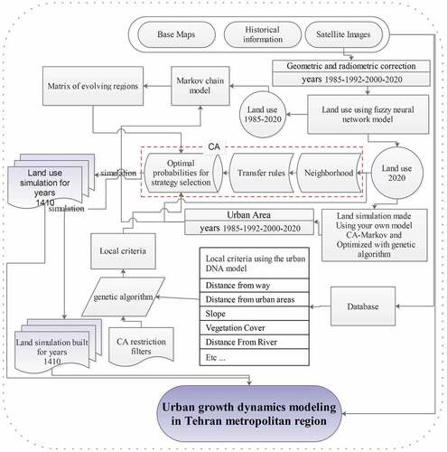
According to the conformity of the results of the analysis of land uses with reality, 96% of the results of the analysis corresponded to reality, which shows the 96% accuracy of the analysis the acceptance of the research results. Figure 4 shows the methodology of the diagram.

Figure 4. Methodological Diagram.

Data

The coverage and land use maps help to quantify and analyse the changes at urban areas. Thus, the TEM+ETM images of Landsat satellite were used at 1985, 1992, 2000 and 2020 years; Due to the use of satellite images with a resolution of 30 metres, the maps have a resolution of 30 metres. FUZZY ARTMAP model was used to generate the land use of this metropolitan. FUZZY ARTMAP is a neural network represented by Carpenter et al. The results of satellite images using FUZZY ARTMAP neural networks in 1985 show that the constructed areas exceeding 60,000 hectares consist of 5% of Tehran metropolitan area. The vegetation is about 145,000 hectares which is 12.2% of total area. The industrial area is about 1861 hectares which is 0.48% of total areas. The arid area is the largest class exceeding 983,000 hectares which is 82.2% of total area. Based on results summarized in Table 2, the largest area increase is in an area with 1,197,243 hectares which is a constructed land use with 82,577 hectares increase during recent 35 years. According to Table 3, this increase includes arid lands with 56,254 and then farmlands exceeding 29,318 hectares. The industrial and irrigated lands consist of smaller than 1% of total changes. The most reduction is in arid land with 115,024 hectares. The results are summarized in Table 2 and Figure 5.

Table 2. The Land Use Areas of Tehran City During 1985–2020.

	1985 Area	Percentage	1992 Area	Percentage	2000 Area	percentage	2020 area	percentage
Constructed	60,123.78	5.022	79,948.53	6.67	93,071.88	7.77	142,701.2	11.92
Arid	983,868.7	82.18	985,949.2	82.35	1,002,983	83.77	868,844.4	72.57
Vegetation	145,582	12.16	120,963.1	10.1	89,403.75	7.47	161,322.9	13.47
Irrigation lands	1861.92	0.15	2277.36	0.19	1133.82	0.095	2492.73	0.21
Industrial Areas	5806.62	0.48	8104.86	0.68	10,650.78	0.89	21,881.7	1.83
Total	1,197,243	100	1,197,243	100	1,197,243	100	1,197,243	100

Table 3. The Changes In Land Use Of Tehran Metropolitan During 1985–2020.

	Constructed	Arid	Vegetation	Irrigated Lands	Industrial Areas	2020
Constructed	56,997.45	56,254.86	29,318.04	22.59	108.27	142,701.2
Arid	0	814,519.5	53,454.78	870.12	0	868,844.4
Vegetation	0	100,066.1	61,104.96	151.83	0	161,322.9
Irrigated Lands	0	1640.34	241.56	610.83	0	2492.73
Industrial Areas	3126.33	11,387.79	1462.68	206.55	5698.35	21,881.7
1985	60,123.78	983,868.7	145,582	1861.92	5806.62	1,197,243

Figure 5. The Land Use Map Of Tehran During 1985–2020.

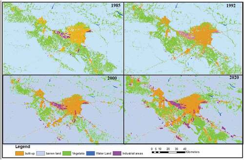
The results indicate that the total pattern of changes in Tehran metropolitan is to increase the constructed area including urban and industrial applications. Contrarily, the arid areas are decreased regarding the cultivation and converting to urban and industrial areas. A notable change is observed based on image processing of satellite images. Is the considerable expansion still the best choice regarding the environmental and ecological concerns?

Increasing growth of construction may lead to miscellaneous side effects such as increasing pollution, decreasing the urban area, increasing the rubbish, increasing the energy and resources consumption.

Main DNAs effective on growth of Tehran metropolitan area

One of critical issues of 21st century scientists includes the city permanency, form of the city and spatial pattern of urban expansion. The form of city is often described as a pattern of spatial expansion in a specific period of time (Anderson, Kanaroglou, and Miller 2001). In recent decades, the suburban areas are shown as the deviation from central areas of cities (Glaeser and Kahn 2004; Helbich and Leitner 2010).

The main sprawl factor is expansion of commercial band as mono purpose with low density and large area, weak accessibility and insufficient public space. Besides, the traffic is one of challenging problems as one of consequences in addition to environmental problems (Jiang and Yao 2010; Arsanjani et al. 2013). Therefore, understanding the growth patterns and motives of urban growth is of a great deal of importance (Deng et al. 2008; Li et al., 2013; Seto et al., 2011; Arsanjani et al. 2013). The urban DNA is a concept that describes the exclusive properties of a city such as topography, soil, and economic situation, social, political, cultural, and environmental indexes (Wu and Silva, 2011). Similar to biological DNA, the main assumption of urban DNA is based on the fact that the main elements existing in a city determine their future growth pattern. Thus, the geographic problems are assessed in an even rearrangement of space with geographic homogeneity. Based on urban growth literature, there are no series of factor which can describe the effective factors on growth and land coverage since each case study has its own specific DNA. Presenting a comprehensive definition for a series of urban DNA is too complicated to describe the urban growth specifically. A city is complicated since many parameters can affect the urban growth. Additionally, different urban DNAs are described based on different programmes and viewpoints. Thus, 13 variables were selected as the factors affecting the urbanization of Tehran metropolitan as independent variables as summarized in Table 4 and Figure 6.

Figure 6. Effective Parameters On Spatial Pattern Of Urban Areas Of Tehran Metropolitan.

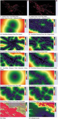
Figure 6. (Continued).

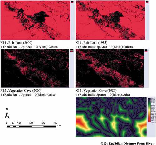
Table 4. Variables Used In Logistic Regression.

Variable Nature	Variable Type	Variable	Code
Boolean	Added Urban Area (1985–2000)	Dependent	Y
Boolean	Added Urban Area (2000–2020)
Continues	Distance From Village	Independent	X1
Continues	Distance From Airport		X2
Continues	Distance From Fault		X3
Continues	Distance from way		X4
Continues	Distance From Industrial Centre (1985)		X5
Continues	Distance From Industrial Centre (2000)
Continues	Distance From Railway Station		X6
Continues	Distance From Main City Downtown		X7
Continues	Distance From Urban Areas(In 2000)		X8
Continues	Distance From Urban Areas (In 1985)
Continues	Altitude Levels		X9
Continues	Slope		X10
Boolean	Bair-Land In 1985		X11
Boolean	Bair-Land In 2000
Boolean	Vegetation Cover in 1985		X12
Boolean	Vegetation Cover in 2000
Continues	Distance From River		X13

Reference: author, 202, Landsat images and cartographic organization maps

Modelling the urban growth dynamics in Tehran metropolitan

About 12,635,000 pixels were randomly selected among 13,303,000 pixels to start the modelling process of expansion of Tehran lands. The total area except the areas constructed at 1985 including arid areas, vegetation and irrigation lands at 1985 were selected at areas with potential possibility of construction at 2020. Each pixel includes a variable of land-use during 1985–2020. Also, the areas constructed during 1985–2020 are considered as dependent variables. Additionally, 13 variables were considered as independent variables as summarized in Table 4. The land-use change factors were weighted from 0 to 1 which indicates that each pixel converted from non-urban to urban during 1985–2020 has the value of 1 while no change is correspondent to 0. The data were used to form a logistic regression model. The obtained parameters were used as a possible solution to generate the appropriate function in genetic model and starting the optimization process. Thus, the genetic algorithm was applied to consider the probability of conversion of cell from non-urban to urban as shown in Tables 5–6.

Table 5. Coefficients Obtained From Regression And Genetic Of Urban Growth During 1985–2020.

1985–2020
GA	Logistic	Variable Nature	Variable Type	Code
−4.43004	−5.0275062		(Intercept)
0.896572	0.00018109	Connected	Distance From Village	X1
−0.59405	−0.00000043	Connected	Distance From Airport	X2
0.944311	0.00003542	Connected	Distance From Fault	X3
−0.61657	−0.00029128	Connected	Distance From Way	X4
−0.32357	−0.00005773	Connected	Distance From Industrial Areas 1985	X5
−0.31128	−0.00000073	Connected	Distance From Railroad Station	X6
−0.4411	−0.00002469	Connected	Distance From City Centre	X7
−0.24561	−0.00010804	Connected	Distance From Urban Points	X8
0.936829	0.0066924	Connected	Elevation levels	X9
−0.42781	−0.69998621	Connected	Slope	X10
9.285766	6.15372472	Boolian	Arid Areas 1985	X11
9.630308	6.32619061	Boolian	Vegetation	X12
−0.37647	−0.00001695	Connected	Distance From River	X13

Table 6. Precision of Forecast By GA-CA Model For Different Periods In Tehran Metropolitan Area.

Forecast precision	Period
98.10	1985–1992
96.83	1985–2000
93.16	1985–2020

Based on the obtained results from optimum chromosome of GA (for example, the optimum parameters of CA), the effect of different parameters is shown on changes of other lands to urban areas in Tehran metropolitan areas. According to Tables 5–6, the effect of parameters including 13 factors is shown based on the urban DNAs of Tehran from non-urban to urban land use conversion. As can be seen, the negative value shows a high probability to convert a non-urban cell into an urban one. Similarly, a positive value shows lower probability to change of non-urban cell into an urban one at next time period. Therefore, a map of independent variable and urban expansion was produced as the dependent variable during 1985–2000 based on the results summarized in Tables 5–6. Among 13 variables, 5 variables including distance from villages, distance from fault, elevation levels, arid areas and vegetation had a direct relation with urban expansion. According to obtained results, the urban growth is mainly observed on arid areas and vegetation. Considering the fault and rural areas, the results indicate that the tendency towards urban expansion is increased as the distance from village is increased. Also, as the elevation level is increased, the tendency towards urban expansion is increased during 1985–2000. Among 13 variables, 8 variables including distance from road, distance from industrial areas, and distance to railroad, distance to city centre, distance to airport, slope, and distance to river have depressive effect on urban expansion. Roads and appropriate accessibility are fascinating parameters which affect the urban expansion which shows the growth of urban areas in interurban roads which changes the urban shape as radial. Considering the urban centre, the negative relation shows the tendency of urban expansion in areas near the urban. The tendency to urban expansion is decreased as the distance from railway station and airport is increased since the citizens tend to be provided with advantages of facilitated transportation. As expected, the tendency towards areas with lower slope always higher which is in agreement with obtained results. Similar findings are expected with the distance from river. Based on GA-CA algorithm modelling, the land use of 1985 was applied as input with a series of transition rules optimized by GA to simulate the urban growth pattern. Each year was considered as repeat during 1985 to 2020. Therefore, the land use of 2020 was repeated after 35 cycles. Two statistical and apparent methods were used to assess and consider the reliability of output of models. The predicted maps were matched with 1992, 2000 and 2020 maps in MATLAB software comparing the formed pixels in land-use map at a given year showing that the GA-CA method is accurate and obtained results are reliable as shown in Table 6.

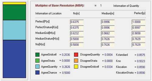
The reliability and assessment of GA-CA algorithm output are of considerable importance to apply the model in modelling the urban expansion of Tehran metropolitan and interpretation of data without proper assessment may be resulted in confusing and ambiguous outcomes. Although numerous methods can be applied to compare the maps statistically, the proposed method should meet the required standard as follows: 1: the interpretation should be straightforward; 2: the presented data help to improve the model; 3: the fundamental question about the similarity of maps should be taken into account. The validate method considers the correspondence of two maps. In this model, a statistical analysis is done to answer two main questions as follows the results including different kappa values determining the consistency and statistical significance between two images (Pontius, 2000: 1012). To this, the 30th cycle map resulted from urban growth model using GA-CA algorithm was compared to 2020 map to validate the accuracy of applied method. The kappa value of this comparison was about 0.932 (Figure 7). The results are summarized in Figure 7. The kappa reported in this work shows that the method is accurate compared to similar works at literature. Also, the obtained kappa from GA-CA shows an improvement of about 5% compared to CA-MARKOV method in this work.

Figure 7. Consistency And Inconsistency Of Real And Simulated Maps At 2020.

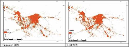
The results of simulation of urban growth at 2020 and its comparison with real map at 2020 are summarized in Figure 8.

Figure 8. Real and Simulated Maps At 2020.

Also, in order to validate the forecast model, in addition to the kappa coefficient, the Figure of Merit coefficient has been used to validate the forecast model. The competency number statistic has a value between 0 and 100. The value of 100 indicates the complete conformity of the predicted map with the terrestrial reality the value of zero indicates the discrepancy. The closer this number is to 100, the higher the accuracy of the forecast (Pontius et al ., 2007).

$\mathrm{F}\mathrm{O}\mathrm{M}=\left(\frac{\mathrm{B}}{\mathrm{A}+\mathrm{B}+\mathrm{C}}\right)$

A: The number of pixels that have actually changed but remained constant in forecast: Means pixels that have changed in terrestrial reality but have remained constant in forecast.

B: It means the number of pixels that have remained constant in terrestrial reality, but these pixels have remained constant in the model forecast:

C: According to the results obtained, the CA_GA forecast model shows a relatively good merit number of about 42%.

According to evaluation of modelling methods, one important question is what is the best method for the urban growth simulation? Considering the input data, the ANN, CA, logistic regression and base operating models, etc. are widely used that provide a variety of results. However, when modelling the urban growth dynamics, the CA approach is adopted as a development tool, especially when integrated with geographical information system (GIS). At the same time, CA systems are considered as a suitable tool for exploring a wide range of major theoretical issues in urban growth dynamics and evaluation.

Accordingly, in this study, modelling includes the CA urban expansion model that has been linked to an optimization unit using a genetic algorithm to search for the optimum set of transition rules and parameters. Then, applying the CA model, a set of optimum rules and parameters is utilized to simulate the dynamics of the urban expansion process. The results obtained from optimum chromosome genetic algorithm (for instance, the optimum set of CA parameters) in fact reflect the effects of various factors including 13 criteria on the change of land-use from non-urban to urban in Tehran metropolitan region, given the urban DNAs of Tehran metropolitan region.

Based on the findings, the increase in the negative parameters signifies the higher probability of converting a cell from non-urban into urban. Likewise, a positive parameter signifies the lower probability for a non-urban cell to be changed into an urban one in a later period. Accordingly, using the GA-CA simulation algorithm, the 1985 land-use map was used as primary input data with a set of land use transfer rules optimized by GA for simulation. Validating the GA-CA self-adaptive algorithm and evaluating its output is of high importance for its application to modelling the urban land expansion in the Tehran metropolitan region. More precisely, the model interpretation without proper validation can lead to misleading results.

As the comparison results between the real and simulated maps indicate, the overall forecast precision for 2020 based on the kappa value is 0.932. According to the detailed results on the validation method performed in this study and other similar works, this degree of precision provides the required confidence to use the combined GA-CA method for the urban growth simulation.

As compared to the results reported in the national and international research, the kappa coefficient in the modelling shows an acceptable increase. Also, the kappa coefficient obtained from the GA-CA method was higher than the CA-MARKOV method performed in this study by about 5%, which is a very acceptable increase for modelling the urban growth. The results of urban growth simulation compared to other similar national and international research have been presented in Table 6.

Having evaluated the results of urban growth at 2020 and proving the efficacy of self-consistent GA-CA method, the simulated map was simulated again for 2030. To this, the maps of 1985, 1992, 2000 and 2020 (Figure 5) were used; the simulation was carried out through some transition rules by GA as shown in Tables 5–6. The results indicate that the urban areas will exceed 214,000 hectares. The maps obtained are depicted in Figures 9 & 10.

Figure 9. The Simulated Map Using GA-CA Model At 2030.

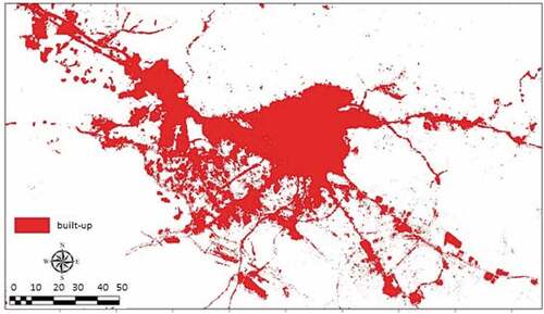
Figure 10. Increase and Decrease of Land Use In The Metropolis Of Tehran During The Years 2020–2030 (Hectares).

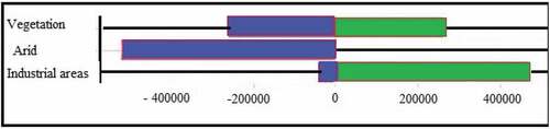
The highest increase is related to the constructed lands and then to the vegetation. But in orchards and agricultural lands, it has decreased almost as much as it was added to these lands during this 15-year period (Figure 10); which indicates the degradation of quality land and their conversion into built lands, and consequently due to the decrease in production and increase in demand for agricultural and horticultural products due to the increase in population in the study area, the conversion of low value and low-yield land to it is a garden and agricultural land. Therefore, in the future expansion of urban areas, attention should be paid to this issue the least amount of destruction should be done in agricultural and garden lands in the urban area of Tehran.

Conclusion

The urban growth dynamics is of critical importance in new world. The similar results considering the urban expansion verifies the increasing urban growth in main areas especially the under-developed country (Table 7). (Forman, 1995; Galster et al. 2001; Heimlich and Anderson 2001; Wasserman 2000; Wilson et al. 2003, MacDonald and Rudel, 2005; Wang et al. 2003; Weng, Liu, and Lu 2007; Wilson et al. 2003; Herold et al., 2005; Hedblom and Soderstrom 2008; Bhatta 2008). Regarding the fact that the urban DNA is exclusive, no one can present a comprehensive pattern including all affecting factors on urban growth process. Thus, 13 effective variables were considered in spatial pattern of Tehran metropolitan (Table 8). A wide range of factors are considered for better understanding the affecting parameters compared to methods and analysis carried out at literature. Among 13 variables, five independent variables including distance from villages, distance from fault, elevation levels, arid areas and vegetation have positive effect on urban expansion. Also, eight variables including the distance from road, distance from railroad station, distance from city centre, distance from urban points, distance from airport, slope, and distance from river showed a negative relation indicating that increasing these factors reduces the urban expansion.

Table 7. Precision of the results related to urban growth simulation in national and international research.

Domestic Research		Foreign Research
Author	Precision	Author	Precision
Barredo et al. (2004)	.88		.87
Chunyang et al. (2006)	.86		.81
He et al. (2006)	.80	Mohammadi et al. (2013)	.89
He et al. (2008)	.86	Heidariyan et al. (2015)	.89
Yang et al. (2008)	.87		.87
	.87	Hosseini et al. (2019)	.89
	.88
	.82
Shafizadeh Moghadam & Helbich (2013)	.86
	.78
	.82
	.89
	.91
Lakshmi and Yarrakula (2016)	.8

Table 8. Studies Related To Effective Factors on Urban Growth Dynamics.

Assessment factors	Distance To River	Distance From Railload	Distance From Railroad	Distance From Airport	Distance from City Centre	Social Factors	Slope	Elevation	Environmental Factors	Risky Lands	Farm Lands	Appropriate For City	Regional Classification	Population Density	Land Value	Distance From River	Distance From Cbd	Arid Areas	Urban Edge
Deadman et al. (1993)	*									*	*
Clarke et al. (1997)	*						*		*				*
Engelen et al. (1999)												*	*
Yeh and Li (2000)												*
Yeh and Li 2001, Yeh and Li 2002)					*				*
Sui and Zeng (2001)	*				*		*	*
Li and Yeh (2002)	*	*			*				*
Almeida et al. (2003, 2013)	*				*									*		*
Barredo et al. (2003, Barredo et al. 2004)	*											*	*
Yeh and Li (2003)	*	*			*						*
Cheng and Masser (2003)	*				*								*	*
Li and Yeh (2004)	*	*			*		*				*
Caruso et al. (2005)	*					*			*
Lau and Kam (2005)	*					*						*		*	*
He et al. (2006)	*	*		*			*		*				*
He et al. (2008)	*	*		*	*		*		*				*
Li et al. (2008)	*	*			*
Liu, Nishiyama, and Yano (2008)	*	*			*			*	*		*
Shan et al. (2008)	*													*
Yang et al. (2008)	*	*			*
Al-kheder et al. (2008)	*						*	*						*
Al-Ahmadi et al. (2009)	*				*	*	*	*
	*				*	*	*						*
	*					*	*	*						*	*	*
Aniekan et al. (2012)	*	*			*	*										*	*
Arsanjani et al. (2013)	*				*	*	*	*			*			*		*	*	*
Shu et al. (2014)	*				*						*		*			*			*
	*	*	*			*	*	*						*	*	*	*	*
	*	*	*			*									*	*	*
Hosseini (2019)	*	*	*	*	*		*	*	*	*	*	*		*	*	*	*	*	*

The present study was carried out to evaluate the effective parameters on urban growth rate to encounter the consequences of future development based on considered factors and specific studied urban DNA. The transition rules were applied to predict the urban growth through GA-CA algorithm during 1985–2020 periods and validating the efficiency of self-consistent method with kappa coefficient of about 93%. The predicted trend was used to simulate the urban growth trend at 2030 through genetic algorithm. The results indicate that the urban growth rate of Tehran will result in expanding urban areas up to 214,000 hectares. The urban expansion results during 1985–2030 show that the constructed areas is increased 2.5 times during a period of 45 years and reaches 214,000 hectares at 2030 while it has been 66,000 hectares in 1985.

Based on theoretical interpretation of obtained results, it can be concluded that the urban growth is a very complicated process and is resulted from interplay between miscellaneous affecting factors. The self-consistent GA-CA model was applied, regarding the limits of CA model to calibrate the transition rules, to monitor the urban expansion pattern which shows an improvement compared to similar conventional algorithms.

Therefore, what can be considered here are the similar results that result from the rapid growth of urban areas according to the patterns and processes related to the spatial organization of metropolitan areas in all urban areas of the world and especially in developing countries. It is also similar to many studies around the world (for example: Forman, 1995; Galster et al. 2001; Heimlich and Anderson 2001; Wasserman 2000; Wilson et al. 2003; Galster et al. 2001; Wang et al. 2003; Weng, Liu, and Lu 2007; Wilson et al. 2003; Hedblom and Soderstrom 2008; Bhatta 2008).

However, based on the accuracy assessment compared to other similar studies, this level of accuracy provides the necessary assurance about using the combined GA-CA method to simulate urban growth) (He et al. 2006; Liu and Yang 2008). However, in this study, urban growth modelling in the metropolitan area of Tehran with respect to the components that form this metropolis both in terms of force and in terms of motivating factors and how to expand urban areas in this metropolitan area according to the components affecting it has been evaluated. However, in this study, due to the limitations of the analysis (e.g. remote sensing data, census), there may be a wide range of variables that can explain patterns of urban sprawl. In this study, according to the research topic of the existing limitations, only a few limited variables were studied to describe the spatial organization of urban areas in the metropolitan area of Tehran. So given that there is a sufficient domain to include more variables. In future studies, researchers can use the underlying and affective variables in this field to explain the behaviour of metropolitan areas in the country.

Disclosure statement

No potential conflict of interest was reported by the author(s).

References

- Acioly, C. C., and F. Davidson. 1996. “Density in Urban Development.” Building Issues 8 (3): 3–25.
- Al-Ahmadi, K., L. See, A. Heppenstall, and J. Hogg. 2009. “Calibration of a Fuzzy Cellular Automata Model of Urban Dynamics in Saudi Arabia.” Ecol. Complex 6 (2): 80–101. doi:10.1016/j.ecocom.2008.09.004.
- Al-kheder, S., Wang, J., Shan, J., 2008. Fuzzy inference guided cellular automata urban-growth modelling using multi-temporal satellite images. Int. J. Geogr. Inform. Sci. 22 (11–12), 1271–1293.
- Almeida, C. M., M. Batty, A. M. V. Monteiro, G. Camara, B. S. Soares-Filho, G. C. Cerqueira, and C. L. Pennachin. 2003. “Stochastic Cellular Automata Modeling of Urban Land Use Dynamics: Empirical Development and Estimation.” Computers, Environment and Urban Systems 27: 481–509.
- AlmeidaLi, C., J. Li, and J. Wu. 2013. “Quantifying the Speed, Growth Modes, and Landscape Pattern Changes of Urbanization: A Hierarchical Patch Dynamics Approach.” Landscape Ecology 28 (10): 1875–1888.
- Anderson, W. P., P. S. Kanaroglou, and E. J. Miller. 2001. “Urban Form, Energy and the Environment: A Review of Issues, Evidence and Policy.” Urban Studies 33 (1): 7–35. doi:10.1080/00420989650012095.
- Aniekan, E., O. Dupe Nihinlola, N. Peter, M. I. Onuwa Okwuashi, and D. Udoudo. 20122012. ”Modelling and Predicting Future Urban Expansion of Lagos, Nigeria from Remote Sensing Data Using Logistic Regression and GIS.” International Journal of Applied Science and Technology 2 (5,): 116–124.
- Arsanjani, J., M. Helbich, W. Kain, and A. Darvishi Boloorani. 2013. “Integration of Logistic Regression, Markov Chain and Cellular Automata Models to Simulate Urban Expansion.” International Journal of Applied Earth Observation and Geoinformation 21: 265–275. doi:10.1016/j.jag.2011.12.014.
- Barnes, K. B., J. M. Morgan III, M. C. Roberge, and S. Lowe (2001). Sprawl Development: Its Patterns, Consequences, and Measurement. A white paper, Towson University. URL: http://chesapeake.towson.edu/landscape/urbansprawl/download/Sprawl_white_paper.pdf.
- Barredo, J. I., M. Kasanko, N. McCormick, and C. Lavalle. 2003. “Modelling Dynamic Spatial Processes: Simulation of Urban Future Scenarios Through Cellular Automata.” Landsc. Urban Plann 64: 145–160.
- Barredo, J. I., L. Demicheli, C. Lavalle, M. Kasanko, and N. McCormick. 2004. “Modelling Future Urban Scenarios in Developing Countries: An Application Case Study in Lagos, Nigeria.” Environment and Planning B 31: 65–84. doi:10.1068/b29103.
- Batty, M., and P. Longley. 1994. 4 Fractal Cities. A Geometry of Form and Function. London: Academic Press.
- Batty, M., and Y. Xie. 1996. “Preliminary Evidence for a Theory of the Fractal City.” Environment and Planning A 28 (10): 1745–1762. doi:10.1068/a281745.
- Batty, M., and Y. Xie. 1997. “Possible Urban Automata.” Environ. Plann. B: Plann. Design 24: 175–192.
- Batty, M., Y. Xie, and Z. Sun. 1999. “Modeling Urban Dynamics Through GIS-Based Cellular Automata.” Computers, Environment and Urban Systems 23: 205–233.
- Bhatta, B. 2008. Remote Sensing and GIS. New York and New Delhi: Oxford University Press.
- Brueckner, J. K. 2000. “Urban Sprawl: Diagnosis and Remedies.” International Regional Science Review 23 (2): 160–171. doi:10.1177/016001700761012710.
- Caruso, G., Rounsevell, M., Cojocaru, G., 2005. Exploring a spatio-dynamic neighbourhood-based model of residential behaviour in the Brussels periurban area. Int. J. Geogr. Inform. Sci. 19 (2), 103–123.
- Cheng, J., and I. Masser. 2003. “Urban Growth Pattern Modeling: A Case Study of Wuhan City, PR China.” Landscape and Urban Planning 62: 199–217. doi:10.1016/S0169-2046(02)00150-0.
- Chunyang, H., P. Shi, J. Li, J. Chen, Y. Pan, J. Li, and T. Ichinose. 2006. “Restoring Urbanization Process in China in the 1990s by Using Non-Radiance-Calibrated DMSP/OLS Nighttime Light Imagery and Statistical Data.” Chinese Science Bulletin 51 (13): 1614–1620.
- Clarke, K. C., S. Hoppen, and L. Gaydos. 1997. “A Self-Modifying Cellular Automaton Model of Historical Urbanization in the San Francisco Bay Area.” Environ. Plann. B: Plann. Design 24: 247–261.
- Clarke, K. C., and L. J. Gaydos. 1998. Loose-Coupling a Cellular Automaton Model and GIS: Long-Term Urban Growth Prediction for San Francisco andWashington/baltimore. International.
- Couclelis, H. 1997. “From Cellular Automata to Urban Models: New Principles for Model Development and Implementation.” Environment and Planning. B, Planning & Design 24 (2): 165–174.
- Deadman, P., R. D. Brown, and H. R. Gimblett. 1993. “Modelling Rural Residential Settlement Patterns with Cellular Automata.” Journal of Environmental Management 37: 147–160.
- Deng, X., J. Huang, S. Rozelle, and E. Uchida. 2008. “Growth, Population and Industrialization, and Urban Land Expansion of China.” Journal of Urban Economics 63: 96e115. doi:10.1016/j.jue.2006.12.006.
- Dubovyk, O., R. Sliuzas, and J. Flacke (2010). Spatial-Temporal Analysis of Informal Settlements Development: A Case Study in Istanbul, Turkey. Conference Proceeding of EARSeL Joint SIG Workshop: Urban 3D Radar Thermal Remote Sensing and Developing Countries. At Ghent.
- Engelen, G., S. Geertman, P. Smits, and C. Wessels, S. Stillwell, S. Geertman, S. Openshaw 1999. ”Dynamic GIS and Strategic Physical Planning Support: A Practical Application to the Ijmond/zuidkennemerland Region.” In Geographical Information and Planning, edited by S. Stillwell, S. Geertman, S. Openshaw Berlin: Springer-Verlag.
- Fogel, D. B. 2000. What Is Evolutionary Computation?, 26–32. IEEE Spectrum.
- Forman, R. T. T. 1995. Land Mosaics: The Ecology of Landscapes and Regions. Cambridge: Cambridge University Press.
- Frumkin, H. 2002. “Urban Sprawl and Public Health.” Public Health Reports 117: 201–217. doi:10.1016/S0033-3549(04)50155-3.
- Galster, G., R. Hanson, H. Wolman, S. Coleman, and J. Freihage. 2001. “Wrestling Sprawl to the Ground: Defining and Measuring an Elusive Concept.” Housing Policy Debate 12 (4): 681–717. doi:10.1080/10511482.2001.9521426.
- Geymen, A., and I. Baz. 2008. “Monitoring Urban Growth and Detecting Land-cover Changes on the Istanbul Metropolitan Area.” Environmental Monitoring Assessment 136: 449–459. doi:10.1007/s10661-007-9699-x.
- Glaeser, E. L., and M. E. Kahn. 2004. “Sprawl and Urban Growth.” In The Handbook of Urban and Regional Economics, edited by V. Henderson and J. Thisse, 1523. Oxford: Oxford University Press.
- Grimm, N. B., J. M. Grove, S. T. A. Pickett, and C. L. Redman. 2000. “Integrated Approaches to Long-term Studies of Urban Ecological Systems.” BioScience 50: 571–584. doi:10.1641/0006-3568(2000)050[0571:IATLTO]2.0.CO;2.
- Grimm, N.B., S.H. Faeth, N.E. Golubiewski, Redman, C.L., Wu, J., Bai, X., & Briggs, J.M. 2008. ”Global Change and the Ecology of Cities”. Science 319: 756–760. doi:10.1126/science.1150195.
- He, C., N. Okada, Q. Zhang, P. Shi, and J. Zhang. 2006. “Modeling Urban Expansion Scenarios by Coupling Cellular Automata Model and System Dynamic Model in Beijing, China.” Applied Geography 26: 323–345. doi:10.1016/j.apgeog.2006.09.006.
- He, C., N. Okada, Q. Zhang, P. Shi, and J. Li. 2008. “Modelling Dynamic Urban Expansion Processes Incorporating a Potential Model with Cellular Automata.” Landsc. Urban Plann 86: 79–91.
- Hedblom, M., and B. Soderstrom. 2008. “Woodlands across Swedish Urban Gradients: Status, Structure and Management Implications.” Landscape and Urban Planning 84: 62–73. doi:10.1016/j.landurbplan.2007.06.007.
- Heimlich, R. E., and W. D. Anderson. 2001. “Development at the Urban Fringe and Beyond: Impacts on Agriculture and Rural Land.” ERS Agricultural Economic Report 1 (803): 88.
- Heimlich, R.E. and Anderson, W.D. (2001). Development at the Urban Fringe and Beyond: Impacts on Agriculture and Rural Land. ERS Agricultural Economic Report No. 803, p. 88.
- Helbich, M., and M. Leitner. 2010. “Postsuburban Spatial Evolution of Vienna’s Urban Fringe: Evidence from Point Process Modeling.” Urban Geography 31 (8): 1100–1117. doi:10.2747/0272-3638.31.8.1100.
- Herold, M., H. Couclelis, and K. C. Clarke. 2005. “The Role of Spatial Metrics in the Analysis and Modeling of Urban Change.” Computers, Environment and Urban Systems 29: 339–369.
- Heydarian, P., K. Rangzan, S. Maleki, and A. Taghi Zadeh. 2016. “Modeling Urban Development Using Statistical Preprocessing Techniques and Artificial Neural Network: The Case of Tehran Metropolis.” Geography and Environmental Planning 26 (4): 97–118.
- Hosseini, S. A., M. Modiri, S. Mishani, and M. H. Heidar. 2015. “Evaluation and Optimization of Tehran’s Urban Sprawl Using GIS and RS.” Annals of the Brazilian Academy of Sciences 87 (1): 72–80. doi:10.1590/0001-3765201521566178.
- Hosseini, S., and A. 2019. ”Explaining the Effective Factors on Spatial Organization of City's in Tehran Metropolitan Region.” Geographi. The University of Sistan & Baluchestan.
- Hu, Z., and C. P. Lo. 2007. “Modeling Urban Growth in Atlanta Using Logistic Regression.” Computers, Environment and Urban Systems 31: 667–688. doi:10.1016/j.compenvurbsys.2006.11.001.
- Huang, S. L., C. T. Yeh, and L. F. Chang. 2009. “The Transition to an Urbanizing World and the Demand for Natural Resources.” Current Opinion in Environmental Sustainability 2 (3): 136–143. doi:10.1016/j.cosust.2010.06.004.
- Jacquin, A., L. Misakova, and M. Gay. 2008. “A Hybrid Object-based Classification Approach for Mapping Urban Sprawl in Periurban Environment.” Landscape and Urban Planning 84: 152–165. doi:10.1016/j.landurbplan.2007.07.006.
- Jiang, B., and X. Yao, Eds. 2010. Geospatial Analysis and Modelling of Urban Structure and Dynamics. Dordrecht, The Netherlands: Springer.
- Kanaroglou, P. S., and D. M. Scott. 2016. “Integrated Urban Transportation and Land-use Models.” In Governing Cities on the Move: Functional and Management Perspectives on Transformations of European Urban Infrastructures, edited by M. Dijst, W. Schenkel, and I. Thomas, 42–72. Aldershot: Ashgate.
- Lakshmi, E. S., and K. Yarrakula. 2016. “Monitoring Land Use Land Cover Changes Using Remote Sensing and GIS Techniques: A Case Study Around Papagni River, Andhra Pradesh, India.” The Indian Ecological Society 43 (2): 383–387.
- Langton, C. 1986. “Studying Artificial Life with Cellular Automata.” Physica D 22: 120–149. doi:10.1016/0167-2789(86)90237-X.
- Lau, K. H., and B. H. Kam. 2005. “A Cellular Automata Model for Urban Land-Use Simulation.” Environ. Plann. B: Plann. Design 32: 247–263. doi:10.1068/b31110.
- Li, X., and A. G. O. Yeh. 2004. “Data Mining of Cellular Automata’s Transition Rules.” Int. J. Geogr. Inform. Sci 18 (8): 723–744.
- Li, C., J. Li, and J. Wu. 2013. “Quantifying the Speed, Growth Modes, and Landscape Pattern Changes of Urbanization: A Hierarchical Patch Dynamics Approach.” Landscape Ecology 28 (10): 1875–1888. doi:10.1007/s10980-013-9933-6.
- Liu, J. G., and P. J. Yang. 2008. Essential Image Processing and GIS for Remote Sensing, 450. New York: Wiley-Blackwell.
- Liu, Y., S. Nishiyama, and T. Yano. 2008. “Analysis of Four Change Detection Algorithms in Bi-temporal Space with a Case Study.” International Journal of Remote Sensing 25: 2121–2139. doi:10.1080/01431160310001606647.
- Luck, M., and J. Wu. 2002. “A Gradient Analysis of Urban Landscape Pattern: A Case Study from the Phoenix Metropolitan Region, Arizona, USA.” Landscape Ecology 17 (4): 327–339. doi:10.1023/A:1020512723753.
- MacDonald, K., and T. K. Rudel. 2005. “Sprawl and Forest Cover: What is the Relationship?.” Applied Geography 25 (1): 67–79.
- Mitchell, J. G. 2001. “Urban Sprawl: The American Dream?” National Geographic 200 (1): 48–73.
- Mohammadi, M., E. Malekipour, and A. Sahebgharani. 2013. “Modeling Urban Expansion in Pripheral Lands Through Cellular Automata (CA) and Analytic Hierarchichal Process.” Case Study of Isfahan’s 7th Municipal District 5 (18): 175–192.
- Nelson, A. C., and T. Moore. 1993. “Assessing Urban Growth Management—the Case of Portland, Oregon.” Land Use Policy 10 (4): 293–302. doi:10.1016/0264-8377(93)90039-D.
- Newman, P. W. G., and J. R. Kenworthy. 1988. “The Transport Energy Trade-off: Fuel-efficient Traffic versus Fuel-efficient Cities.” Transportation Research A 22A (3): 163–174. doi:10.1016/0191-2607(88)90034-9.
- Ning, W., and E. A. Silva. 2011. ”Urban DNA: Exploring the Biological Metaphor of Urban Evolution with DG-ABC Model.” Agile . 1–7.
- O’Sullivan, D., and P. M. Torrens. 2000. “Cellular Models of Urban Systems.” In Theoretical and Practical Issues on Cellular Automata, edited by S. Bandini and T. Worsch, 108–116. London: Springer.
- Openshaw, S., and C. Openshaw. 1997. Artificial Intelligence in Geography. New York. USA: John Wiley & Sons, .
- Páez, A., and D. M. Scott. 2004. “Spatial Statistics for Urban Analysis: A Review of Techniques with Examples.” GeoJournal 61 (1): 53–67. doi:10.1007/s10708-005-0877-5.
- Pontius, J., and R. Gilmore. 2000. “Quantification Error versus Location Error in Comparison of Categorical Maps.” Engineering and Remote Sensing 66 (8): 1011–1016.
- Pontius G. R., Walker, R., Kumah, R., Arima, E., Aldrich, S., Caldad, M. and Vergara, D., 2007. Accuracy assessment for a simulation model of Amazonian deforestation. Annals of the American Association of Geographers. 97, 677–695
- Rienow, A., and R. Goetzke. 2014. “Supporting SLEUTH – Enhancing a Cellular Automaton with Support Vector Machines for Urban Growth Modeling, Computers.” Environment and Urban Systems xxx: 1–16.
- Robert, H. S. 2013. “Complexity, the Science of Cities and Long-range Futures.” Futures 47: 49–58. doi:10.1016/j.futures.2013.01.006.
- Santé, I., A. M. García, D. Miranda, and R. Crecente. 2010. “Cellular Automata Models for the Simulation of Real-world Urban Processes: A Review and Analysis.” Landscape and Urban Planning 96: 108–122. doi:10.1016/j.landurbplan.2010.03.001.
- Savitch, H. V., D. Collins, D. Sanders, and J. Markham. 1993. “Ties that Bind: Central Cities, Suburbs and the New Metropolitan Region.” Economic Development Quarterly 7 (4): 341–357. doi:10.1177/089124249300700403.
- Seto, K. C., M. Fragkias, B. Guneralp, and M. K. Reilly. 2011. “A Meta-Analysis of Global Urban Land Expansion.” PLoS ONE 6: e23777. doi:10.1371/journal.pone.0023777.
- ShafizadehMoghadam, H., and M. Helbich. 2013. “Spatiotemporal Urbanization Processes in the Megacity of Mumbai, India: A Markov Chains-Cellular Automata Urban Growth Model.” Applied Geography 40: 140–149.
- Shan, J., S. Al-Kheder, and J. Wang. 2008. “Genetic Algorithms for the Calibration of Cellular Automata Urban Growth Modeling.” Photogram. Eng. Remote Sens 74 (10): 1267–1277. doi:10.14358/PERS.74.10.1267.
- Shu, B. Honghui Zh., Yongle Li, Yi Qu, Lihong Ch. (2014). Spatiotemporal variation analysis of driving forces of urban land spatial expansion using logistic regression: A case study of port towns in Taicang City, China. Habitat International. 43: 181–190.
- Silva, E. A. 2001. “The DNA of Our Regions.” In Artificial Intelligence in Regional Planning. World Planning Schools Congress (Paper 5019). Shanghai.
- Silva, E. A., and K. C. Clarke. 2002. “Calibration of the SLEUTH Urban Growth Model for Lisbon and Porto, Portugal.” Computers, Environment and Urban Systems 26: 525–552. doi:10.1016/S0198-9715(01)00014-X.
- Silva, E. A. 2004. “The DNA of Our Regions: Artificial Intelligence in Regional Planning.” Futures 36 (10): 1077–1094. doi:10.1016/j.futures.2004.03.014.
- Silva, E. A., and K. Clarke. 2005. “Complexity, Emergence and Cellular Urban Models: Lessons Learned from Applying SLEUTH to Two Portuguese Cities.” European Planning Studies 13 (1): 93–115. doi:10.1080/0965431042000312424.
- Silva, E. A., (2006) Waves of Complexity: Bifurcations or Phase Transitions, paper presented in IIIRD Meeting of AESOP thematic group on complexity, Cardiff, UK, May.
- Stoel, T. B., Jr. 1999. “Reining in Urban Sprawl.” Environment 41 (4): 6–33.
- Stone, B., Jr. 2008. “Urban Sprawl and Air Quality in Large US Cities.” Journal of Environmental Management 86: 688–698. doi:10.1016/j.jenvman.2006.12.034.
- Sui, D. Z., and H. Zeng. 2001. “Modeling the Dynamics of Landscape Structure in Asia’s Emerging Desakota Regions: A Case Study in Shenzhen.” Landsc. Urban Plann 53: 37–52.
- Syphard, A. D., K. C. Clarke, and J. Franklin. 2005. “Using a Cellular Automaton Model to Forecast the Effects of Urban Growth on Habitat Pattern in Southern California.” Ecological Complexity 2: 185–203. doi:10.1016/j.ecocom.2004.11.003.
- Tseng, L. Y., and S. Yang, (1997) “Genetic Algorithms for Clustering, Feature Selection and Classification”,IEEE Int. Conference on Neural Networks, Korean Institute of Intelligent Systems, 1612–1616.
- Vafaie, H., and I. Imam (1994), “Feature Selection Methods: Genetic Algorithms Vs. Greedy-like Search”. Proc. of the Int. conference on fuzzy and intelligent control systems, Luoisville.
- Verburg, P. H., P. P. Schot, M. J. Dijst, and A. Veldkamp. 2004. “Land Use Modelling Current Practice and Research Priorities.” GeoJournal 61: 309–324. doi:10.1007/s10708-004-4946-y.
- Wang, W., L. Zhu, R. Wang, and Y. Shi. 2003. “Analysis on the Spatial Distribution Variation Characteristic of Urban Heat Environmental Quality and Its Mechanism—a Case Study of Hangzhou City.” Chinese Geographical Science 13 (1): 39–47. doi:10.1007/s11769-003-0083-7.
- Wang, Y., M. Jamshidi, P. Neville, C. Bales, and S. Morain. 2007. “Hierarchical Fuzzy Classification of Remote Sensing Data.” Studies in Fuzziness and Soft Computing 217: 333–350.
- Wasserman, M. 2000. “Confronting Urban Sprawl.” Regional Review of the Federal Reserve Bank of Boston 86: 9–16.
- Webster, C. 1996. “Urban Morphological Fingerprints.” Environment and Planning. B, Planning & Design 23: 279–297.
- Weng, Q., H. Liu, and D. Lu. 2007. “Assessing the Effects of Land Use and Land Cover Patterns on Thermal Conditions Using Landscape Metrics in City of Indianapolis, United States.” Urban Ecosystem 10: 203–219. doi:10.1007/s11252-007-0020-0.
- White, R., and G. Engelen. 1997. “Cellular Automata as the Basis of Integrated Dynamic Regional Modelling.” Environment and Planning B: Planning and Design 24 (2): 235–246.
- White, R., and G. Engelen. 2000. “High Resolution Integrated Modeling of the Spatial Dynamics of Urban and Regional Systems.” Computers, Environment and Urban Systems 24: 383–440. doi:10.1016/S0198-9715(00)00012-0.
- Wilson, E. H., J. D. Hurd, D. L. Civco, S. Prisloe, and C. Arnold. 2003. “Development of a Geospatial.“ Remote Sensing of Environment 86: 275–285. doi:10.1016/S0034-4257(03)00074-9.
- Wu, F., and C. T. Webster. 1998. “Simulation of Land Development through the Integration of Cellular Automata and Multi-criteria Evaluation.” Environment and Planning B 25: 103–126. doi:10.1068/b250103.
- Wu, F., and D. Martin. 2002. “Urban Expansion Simulation of Southeast England Using Population Surface Modeling and Cellular Automata.” Environment and Planning A 34 (10): 1855–1876. doi:10.1068/a3520.
- Wu, X., Y. Hu, H. S. He, R. Bu, J. Onsted, and F. Xi. 2009. “Performance Evaluation of the SLEUTH Model in the Shenyang Metropolitan Area of Northeastern China.” Environmental Modeling & Assessment 14 (2): 221–230. doi:10.1007/s10666-008-9154-6.
- Wu, F. 2010. “Housing Provision under Globalisation: A Case Study of Shanghai.” Environment and Planning A 33 (10): 1741–1764. doi:10.1068/a33213.
- Xiao, J., Y. Shen, J. Ge, R. Tateishi, C. Tang, Y. Liang, and Z. Huang. 2007. “Evaluating Urban Expansion and Land Use Change in Shijiazhuang, China, by Using GIS and Remote Sensing.” Landscape and Urban Planning 75: 69–80. doi:10.1016/j.landurbplan.2004.12.005.
- Xie, Y., and M. Batty. 1996. “Automata-based Exploration of Emergent Urban Form.” Geographical System 4: 83–102.
- Yang, Q., X. Li, and X. Shi. 2008. “Cellular Automata for Simulating Land Use Changes Based on Support Vector Machines.” Computers & Geosciences 34: 592–602.
- Yeh, A. G. O., and X. Li. 2000. “A Constrained CA Model for the Simulation and Planning.“ Environment and Planning 28: 733–753. doi:10.1068/2Fb2740.
- Yeh, A. G. O., and X. Li. 2001. “Measurement and Monitoring of Urban Sprawl in a Rapidly Growing Region Using Entropy.” Photogrammetric Engineering and Remote Sensing 67 (1): 83–90.
- Yeh, A. G. O., and X. Li. 2002. “A Cellular Automata Model to Simulate Development Density for Urban Planning.” Environment and Planning B 29: 431–450. doi:10.1068/b1288.
- Yeh, A.G.O., and X. Li. 2003. “Simulation of Development Alternatives Using Neural Networks, Cellular Automata, and GIS for Urban Planning.” Photogram. Eng. Remote Sens 69 (9): 1043–1052.
- Zhang, B. 2003. “Application of Remote Sensing Technology to Population Estimation.” Chinese Geographical Science 13: 267–271. doi:10.1007/s11769-003-0029-0.