Individual level spatial-temporal modelling of exposure potential of livestock in the Cove Wash watershed, Arizona

ABSTRACT

Personal exposure studies suffer from uncertainty issues, largely stemming from individual behaviour uncertainties. Built on spatial-temporal exposure analysis and methods, this study proposed a novel approach to spatial-temporal modelling that incorporated behaviour classifications taking into account uncertainties, to estimate individual livestock exposure potential. The new approach was applied in a community-based research project with a Tribal community in the southwest United States to address questions on potential livestock exposure to abandoned uranium mines (AUMs). The study aimed to 1) classify Global Positioning System (GPS) data from livestock into three behaviour subgroups – grazing, travelling or resting; 2) calculate the daily cumulative exposure potential for livestock; 3) assess the performance of the computational method with and without behaviour classifications. Using Lotek Litetrack GPS collars, we collected data at a 20-min-interval for two flocks of sheep and goats during the spring and summer of 2019. Analysis and modelling of GPS data demonstrated no significant difference in individual cumulative exposure potential within each flock when animal behaviours with probability/uncertainties were considered. However, when daily cumulative exposure potential was calculated without consideration of animal behaviour or probability/uncertainties, significant differences among animals within a herd were observed, which does not match animal grazing behaviours reported by livestock owners. These results suggest that the proposed method including behaviour subgroups with probability/uncertainties more closely resembled the observed grazing behaviours. Results from the research may be used for future intervention and policy-making on remediation efforts in communities where grazing livestock may encounter environmental contaminants.

KEYWORDS:

• GPS
• domesticated livestock
• fuzzy logic
• behaviour patterns
• cumulative exposure
• time geography
• GIS
• parallel computing

1. Introduction

Uranium mining began on the Navajo Nation, USA, in February 1944 and peaked between the late 1950s and 1970s (Eichstaedt 1994). It was not until the mid-1980s that the demand of uranium ore declined, and mining activities ended on the Navajo Nation (Fettus and McKinzie 2012). Although uranium mining projects ceased, the effects of uranium extraction did not, as uranium and other metals, metalloids, and radionuclides continued to enter the environment and food chain for animals and humans (Holaday 1969; Brugge and Goble 2002). According to a report by United States Environmental Protection Agency (EPA), after the mining industries cease extraction activities on the Navajo Nation more than 500 mine sites were left abandoned. Fifty-two of these abandoned uranium mine (AUM) sites are situated within the Cove Wash watershed, a Navajo community located in northeastern Arizona. Residents of the Cove Chapter are concerned about human exposures to metal mixtures from the presence of nearby AUMs as well as the health of their livestock.

For AUM sites, the chemical toxicity of uranium and other elements constitute the primary environmental health hazard (Meinrath, Schneider, and Meinrath 2003). Uranium, radon, and arsenic, which are byproducts of the uranium mining process, are hazardous to human health. In different regions, researchers have found that the chemical content near abandoned uranium mines is generally high for these elements (Vaupotić 2001; Mudd 2008; Fijałkowska–Lichwa 2016; Hoover et al. 2017; Yazzie et al. 2020). Previous occupational exposure research indicates that radon inhalation from underground uranium mining is associated with cancer in the lung, bone, and skin (Samet et al. 1984; Gottlieb and Husen 1982; Hornung and Meinhardt 1987; Mulloy et al. 2001). People living in an area close to AUMs may also experience adverse pregnancy outcomes due to AUM contaminant exposure, which is an active area of research for the Navajo Birth Cohort Study (NBCS) (Hoover et al. 2020).

Exposure to contaminants from AUMs may be via respiratory, oral, and dermal routes (Kwan and Schwanen 2018). In general, more soluble compounds are less toxic to the lungs but more toxic to the respiratory system due to easier absorption from the lungs into the blood and transportation to distal organs (Brugge, deLemos, and Oldmixon 2005). The oral toxicity of uranium compounds has been evaluated in several animal species following exposure in drinking water or via grazing (Medina et al. 2020; Bolt et al. 2018). Soil and water contaminated by AUMs are integrated into arable land via numerous environmental pathways and absorbed by perennial pasture plants present on lands that may be used for cropping, grazing, or hunting. Thus, consuming meat from grazing animals may also be a significant heavy metal and radionuclide exposure source (Tannenbaum, Silverstone, and Koziol 1948; Gramss and Voigt 2014; Anke et al. 2009; Zamora et al. 1998). Dermal exposure is related to exposure time, the total area of skin that is exposed, and other physical and physiological conditions (Kurttio et al. 2006). Despite this potential complexity, the chemical toxicity of metals is the primary concern in extant exposure studies (Craft et al. 2004). Thus, this paper is mainly focused on respiratory and oral exposure. In the light of these findings and long-standing community concerns about AUMs, Cove community members requested a study investigating the accumulation of uranium in animal tissue. As a response, this study employed a community-driven approach, leveraging geospatial technology to estimate the cumulative environmental exposure potential for livestock grazing in the Cove Wash watershed.

Geographic information systems (GIS) technology provides powerful tools for assessing potential exposures from AUMs among livestock. Tobler’s first law of geography has revealed a relationship in the spatial dimension – all things are related, but near things are more strongly related than distant ones (Tobler 1970). With this law, researchers could analyse potential exposure to AUMs in different geographic areas using location-based methods. Simple location-based methods could be point-in-polygon, buffering, and other distance functions (Moolgavkar 2000; Barbone et al. 1995; Harrison et al. 1999; Jenelius, Petersen, and Mattsson 2006). Additionally, there are other methods, such as kriging, inverse distance weighting (IDW), regression mapping, etc., to interpolate an exposure map with limited data (Zhan et al. 2018; Gong, Mattevada, and O’Bryant 2014; Leelasakultum and Kim Oanh 2017). However, these methods are limited so GIS-based multi-criteria models (GIS-MCDA), and land-use regression models have been developed and applied to exposure studies (Lin et al. 2020; Ryan and LeMasters 2007; Lu and Fang 2015).

There exists a growing body of literature integrating GPS data, environmental data, and traditional GIS approaches for livestock exposure assessments (Handcock et al. 2009; Augustine and Derner 2013; Wang, Kwan, and Chai 2018). However, these GIS methods are limited since they consider spatial dimensions only and do not address temporal dimensions when applied to livestock studies. As a consequence, the computed exposure estimates may be less accurate. Moreover, existing approaches suffer from uncertainty issues, which usually result from inaccurate or misclassified GPS data or stochastic animal behaviours (Brown 2004). Given the environmental risk map, shown in Figure 1, the total exposure would be the sum of the environmental risk values along a pathway (e.g. E1 = R1+ R2+ R3, where E is the total exposure of an individual and R is environmental exposure risk value at a given location), when only the spatial dimension is considered. However, in a real-world scenario, travel speed differs, and the time spent at different locations might vary. This would result in a higher cumulative exposure if the individual livestock spends a longer time inside an area with higher exposure potential, and vice versa (e.g. E2 = R1+ (T2-T1)*R2+ (T4-T3)*R3, where T is time at a location). Thus, the total exposure could be different for the same route when considering the temporal dimension of livestock behaviour.

Figure 1. Exposure assessment in spatial-temporal dimension (Example equations are listed to demonstrate exposure assessment approaches under different scenarios).

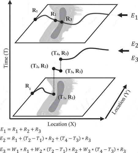
Behaviours have been studied by geographers in many ways. Hägerstrand applied the lifeline concept in demography to study population movement across space, which then matured into the concept of time geography (Hägerstraand 1970). With the advocacy of Hägerstrand and the Lunde School under his leadership, time geography was introduced (Raubal, Miller, and Bridwell 2004). Other research evaluated human behaviours and accessibility to a certain facility (e.g. grocery store, gym, etc.) (Miller 1991; Kwan 1998; Weber 2003). Behaviour information is critical for personal exposure assessment (Kwan and Schwanen 2018). The present manuscript considers behaviour patterns because different behaviours are related to different exposure rates, which might further influence the exposure estimates (e.g. E3 = W1*R1+ W2*(T2-T1)*R2+ W3*(T4-T3)*R3, where Wi represents the weight of different behaviour patterns based on their relative contribution to potential exposure). However, none of the above scenarios consider underlying uncertainties in exposure, including but not limited to: GPS positional accuracy, temporal uncertainty, and livestock behaviour uncertainty; all of which need to be considered for an accurate representation and assessment of exposure (Kim and Kwan 2003).

Early attempts to track animals and record their behaviours were in situ observations. Other methods relied on human observation of natural (e.g. colour patterns) or artificial features (e.g. coloured collar or tag) to identify individual animals. Problems inherent in these methods include observer fatigue and associated error, study area accuracy and physical limitations, other external factors, and observer proximity effects on animals (Meinrath, Schneider, and Meinrath 2003). It has historically been challenging to discern an individual livestock from a herd based on its natural features (such as colour patterns, height, or special spot). Therefore, new methods have been developed to address the above issues, including attaching a physical marker, marking the target animal with stable isotopes, radio tracing. However, disadvantages still exist in such methods, which is the trade-off between accuracy and observer proximity effects (Turner et al. 2000; Rife and Rock 2001).

Modern GPS collars record animal locations at high temporal frequencies, allowing for detection of animal behaviour patterns and interactions between animals and the environment (Allan et al. 2013). Previous studies have overlaid animal locations with land use types to find out frequencies of interaction with different places (Meinrath, Schneider, and Meinrath 2003). For example, if GPS locational points are clustered at two places, of which one is already known to be fenced in and the other is known to be a pasture, it can be inferred how much time animals spend in resting, grazing and other behaviour patterns. Thus, the major livestock behaviours can be specified as: grazing, travelling, and resting. We assume, therefore, that when livestock are grazing, possible exposure routes might involve respiratory, oral, and dermal exposure; when resting, exposure routes might only include oral and respiratory exposure; and when travelling the routes might also contain oral and respiratory exposure. Therefore, it is important to obtain accurate livestock behaviour patterns.

It is a challenging task to completely reproduce the past behaviours of livestock animals at a certain place. Livestock owners may lead a herd to a grazing area from 9:00 AM to 12:00 PM and record the grazing time every day, but an individual livestock may not continually graze during that period. Instead, an individual livestock might spend some time idling or resting. This means that livestock behaviours based on GPS data might involve a number of uncertainties that could be addressed using fuzzy logic. Fuzzy logic is a form of multivalued logic, the output of which can be any real number between 0 and 1, which means the genre of a target is neither A nor B; instead, it can be partially A and partially B at the same time. The key is how much the target belongs to A and how much it belongs to B. Given two sets – input 1 and input 2, fuzzy logic adapts the membership of each input value, for which the membership function is calculated first, followed by predefined fuzzy rules, and classified as an output according to a fuzzy classification. The membership itself represents the likelihood of a certain characteristic (Weston Solutions, Inc 2014; Oren and Ghasem-Aghaee 1998).

The primary research objective of the study is 1) to develop a new approach for spatial-temporal modelling that incorporates automatic livestock behaviour classifications accounting for uncertainties; 2) to calculate the daily cumulative exposure potential for livestock and 3) to assess the performance of the proposed method when compared with previous approaches without behaviour classifications or probability/uncertainties. To answer these questions, we classified livestock behaviour patterns, estimated the cumulative environmental exposure risk for each individual livestock with and without behaviour patterns or probability/uncertainties, and compared the results. The implication of this study is two folds: on the one hand, the proposed method has the potential to produce more accurate exposure analysis results and therefore could have a widespread use in exposure studies; on the other hand, results from this study will help answer questions in a larger ongoing community-based research study on potential human health risks from consuming meat and organs of livestock grazing in the Cove Wash watershed and can therefore inform interventions and remediation efforts to address community environmental health concerns.

2. Data and methods

2.1. Overview of this research

The workflow of this paper is shown in Figure 2. We first collected data with GPS collars to obtain locational and other relevant information of individual livestock at a 20-min interval. Invalid records were removed as discussed in section II-C.

Figure 2. Research workflow including data collection, cleaning and analysis.

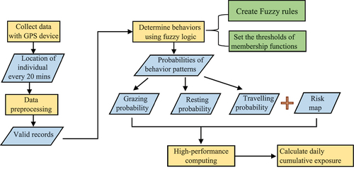
Using valid records, we developed a fuzzy inference system to classify livestock behaviours using Matlab (Version R2020a). We first created the fuzzy rules and defined the thresholds of membership functions. Afterwards, we derived probabilities of three behaviour patterns: grazing, resting and travelling. Details are discussed in section II-D. Potential exposure risk was based on a previously generated environmental risk map covering the Navajo Nation (Kurttio et al. 2006), we uploaded data with behaviour and probability information to the high-performance computers at the University of New Mexico Center for Advanced Research Computing (CARC) with parallel computing capacities to calculate the cumulative environmental exposure (discussed in sections II-E and II-F).

2.2. Study area

The Cove Chapter of the Navajo Nation, with 420 residents (2010 U.S. Census), is situated in the foothills of the Chuska mountain range, tucked away in the Carrizo and Lukachukai mountains in northeastern Arizona. The Cove Wash watershed is in the Northern Agency of the Navajo Nation at the intersection of Utah, Arizona and New Mexico (Figure 3). The watershed contains approximately 52 miles of tributaries and receives about 12–16 inches of precipitation annually. The Cove Wash is an ephemeral stream, which is important when considering how uranium is deposited after rain events. There are 523 AUMs on Navajo Nation – 52 of which are located in Cove.

Figure 3. Distribution of AUMs in Cove.

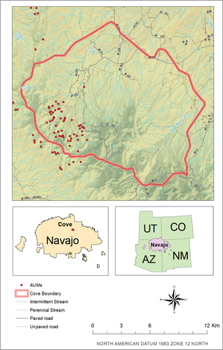
With permission and partnership from livestock owners in the Cove community and Dine College, we attached Lotek GPS collars to livestock (four sheep and four goats) to collect information on location, elevation, and ambient temperature at a 20-min interval. The battery life of the collars could support tracking for up to 1 year. Depending on the flock, tracking time was between 10 days to four months, which was fully determined by livestock owners.

2.3. Data Preprocessing

Some positional records were invalid due to the complex terrain in the watershed blocking signal transmission between satellites and GPS devices or even reflecting the signals before they are received by the devices (an example of collected GPS data is provided in Appendix, Table 5.)

Data were cleaned to remove records that failed to meet the following criteria: 1) duration less than 70 sec; 2) valid latitude and longitude coordinates within the study area; 3) four or more GPS satellites used to record positional information; and 4) elevation greater than 800 m. The duration field reflects the time the GPS receiver takes to connect with all satellites (the maximum time is set by the manufacturer to be 70s). Normally, it takes less than 70 sec for the device to connect to satellites. Larger durations indicate that the device has failed to connect to any satellites and subsequently times out. The satellite field shows how many satellites are connected and used when calculating coordinates. At least four satellites are needed to estimate the 3D position. Thus, GPS data with three or fewer satellites were considered to be invalid. Because the lowest elevation of Cove is over 1000 m, GPS data with altitude below 800 m were also considered invalid.

2.4. Behaviour patterns classification

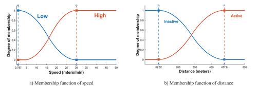
The present workflow uses fuzzy logic to classify different behaviour patterns and the corresponding possibility of each from the GPS data. Fuzzy logic enables inference while allowing for potential alternatives (Zadeh 1965). In this paper, the input variables used for fuzzy classification were speed and the distance to a livestock owner’s house. The speed, calculated using the coordinates and the time stamp, represents the average speed that an individual livestock travels within a 20-min time interval. Membership 1, speed, was used to specify whether the speed is high or low. With a higher value, the chance of moving around or travelling to other places was higher, while the chance of staying at one spot for grazing was lower, and vice versa. Membership 2, status (active or inactive), was used to specify whether distance to the house is large or small. Small distances were considered as ‘inactive zones’, where the animals are most likely inside a corral. Conversely, large distances were considered to be ‘active zones’, where the animals were shepherded outside to graze. The fuzzy rules are shown in Table 1.

Table 1. Fuzzy rules.

Fuzzy Rules	Speed: High		Speed: Low
	Behaviour	Membership	Behaviour	Membership
Status: Inactive	Grazing Resting Travelling	Low Mid High	Grazing Resting Travelling	Low High Low
Status: Active	Grazing Resting Travelling	Mid Low High	Grazing Resting Travelling	High Mid Mid

The membership functions of speed and status are shown in Figure 4. The blue curve in Figure 4 shows the fuzzy membership function of low speed, while the red curve represents that of high speed. The thresholds of speed were confirmed with points geolocated inside the fence and along the road. After conversations with livestock owners, it was clear that the animals were held behind the corral from 00:00 am to 4:00 am next morning, during which point the average recorded speed was 0.787 m per min. When livestock were travelling from the corral to a grazing area, the average speed was 30.12 m per min. Thus, those two values were set as the speed thresholds for high and low values. The blue curve in Figure 4 depicts the membership function of inactive status, while the red curve represents that of active status. The average recorded distance is 82.58 m when the sheep and goats are held inside the fence, but the average distance is 477.6 m when they are out from 9:00 am to 11:00 am. Thus, 82.58 m and 477.6 m were set as the distance thresholds for inactive and active status. With these rules applied, a fuzzy membership score was computed for each valid GPS location.

Figure 4. Membership functions.

a). The blue curve shows the fuzzy membership function of low speed, while the red curve represents that of high speed. b). The blue curve shows the fuzzy membership function of inactive status, while the red curve represents that of active status.

2.5. Cumulative potential exposure

Fuzzy logic is used to derive the degree of occurrence of each behaviour pattern. Even if the probability of one behaviour is higher than the other two behaviour patterns, the possibilities of the other two behaviours resulting from the classification method should be retained.

The potential environmental exposure of a certain behaviour sequence was estimated based on the equation adapted from previous research (Lu and Fang 2015) as below:

(1) $E_j=\underset{t_1}{\overset{t_2}{\int }}\underset{l_1}{\overset{l_2}{\int }}{W}_{i}R\left(t,l\right)dldt$(1)

where W_i represents the weight of the behaviour i based on the relative importance of each behaviour pathway in producing the final exposure potential, and R represents the modelled potential for environmental exposure – a dimensionless value – at location l and time t. The corresponding uncertainty of the behaviour sequence introduced by livestock behaviour classification is quantified into probability:

(2) $P_j=\prod _{\hspace{0.17em}}{P}_B$(2)

where P_B is the probability of certain livestock behaviour derived from fuzzy logic. The uncertainty introduced by modelled potential for environmental exposure is quantified through Monte Carlo Simulation of criteria weights. The cumulative exposure potential was calculated as:

(3) $C_r={\sum }_{j_1}^{j_n}{E}_j{P}_j$(3)

For example, if one animal travels in the time sequence from point A to B and then to C, the corresponding locational exposure level is R₁ at location A, R₂ at location B and R₃ at location C. The exposure map is derived from a GIS-MCDA model that considered multiple physical, environmental, and meteorological inputs, such as proximity to AUM, wind direction, topographic wind exposure, and landform (Lin et al. 2020). For example, locations in close proximity to or downwind of an AUM might have a higher environmental exposure potential when compared with locations upwind or far away. More details about this map could be found elsewhere.

As discussed, an animal may be exposed to environmental toxicants through respiratory, oral intake, and dermal pathways (Moolgavkar 2000). Because the livestock owners in Cove are generally aware of risks associated with AUMs, they tend to avoid or otherwise limit time spent in areas close to AUMs. Also, the skin generally protects deeper tissues from harmful chemicals associated with AUMs (Yazzie et al. 2020). In all, dermal exposure is likely negligible compared to respiratory and oral pathways. However, the mechanisms of respiratory and oral exposures involve the whole-body system, and it remains difficult to quantify the relative influence of each pathway. Thus, this study assumed that respiratory and oral exposure are equally influential. Livestock owners fed their animals hay grown outside Cove and regulated water from their homes when the animals were corralled. From 8 AM to 8 PM, the exposure pathway will be primarily respiratory while resting. The exposure pathway will include both oral intaking and respiratory while grazing. While travelling, the primary exposure pathway is respiratory but with a higher breathing rate. Hence, we assigned the weight of grazing as 2, the weight of resting as 1, and the weight of travelling as 2, considering the relative contribution of each behaviour to exposure.

In theory, the results should have 27 combinations because the animal may graze or rest in all these three places. A demo is shown in Table 2. Then, the daily cumulative environmental exposure risk would be $E=\hspace{0.17em}{C}_1\ast P_1+C_2\ast P_2+\dots +C_{26}\ast P_{26}+C_{27}\ast P_{27}$.

Table 2. Calculation of cumulative risk and probability.

Behaviour combination (G: grazing; R: resting; T: travelling)	Risk ($W_G=2;\hspace{0.17em}{W}_R=1;\hspace{0.17em}{W}_T=2$)	Corresponding possibility
GGG	$C_1=2R_1+2R_2+2R_3$	$P_1=P{G}_A\ast P{G}_B\ast P{G}_C$
GGR	$C_2=2R_1+2R_2+1R_3$	$P_2=P{G}_A\ast P{G}_B\ast P{R}_C$
GGT	$C_3=2R_1+2R_2+2R_3$	$P_3=P{G}_A\ast P{\mathrm{G}}_B\ast P{\mathrm{T}}_C$
.	$.$	$.$
.	$.$	$.$
.	$.$	$.$
RRG	$C_{25}=1R_1+1R_2+2R_3$	$P_{25}=P{R}_A\ast P{R}_B\ast P{G}_C$
RRR	$C_{26}=1R_1+1R_2+1R_3$	$P_{26}=P{R}_A\ast P{R}_B\ast P{R}_C$
RRT	$C_{27}=1R_1+1R_2+2R_3$	$P_{27}=P{R}_A\ast P{R}_B\ast P{\mathrm{T}}_C$

2.6. Parallel computing strategy

The Lotek GPS collars were programmed to collect data every 20 minutes, resulting in 3 GPS points per hour and 72 points per day for each animal prior to data cleaning. We tracked two flocks, A and B, in 2019. We collected 1-month of data for Flock A and 4-months of data for Flock B. The collection periods were determined by livestock owners. In total, there were approximately 2000 points for Flock A and 8000 points for Flock B. Thus, if we were to use one final number to represent the cumulative environmental exposure for an individual livestock, the calculation completeness would be 3²⁰⁰⁰ for Flock A and 3⁸⁰⁰⁰ for Flock B. This amount of computational task was impossible based on current computing capacity. The exponential increase of calculations as input points increase is referred to as the NP-hardness problem (Fortnow 2009). Decreasing the number of selected points is a typical way to overcome such problem. Thus, we converted the above analysis to daily scale. However, even at the daily scale, computing the cumulative exposure potential has 3⁷² calculation completeness, which was still impossible for any current computing recourses. Conversations with livestock owners informed our approach to this computation challenge. We knew that the livestock were corralled daily after 8:00 PM and were not let out until 8:00 AM the next day. Thus, this study only focused on time from 8:00 AM to 8:00 PM. Still, the time completeness of 3³⁶ was too large. We decided to use one out of three GPS points (within every hour) to represent the hourly status of one individual livestock. After reducing the input data, the time completeness was 3¹² per day. However, personal computers are unable to support the full load of such calculation task for a long time, due to restrictions of the power supply system and cooling system and the daily use demand. Data processing was in turn conducted at the University of New Mexico Center for Advanced Research Computing (CARC) where the Python codes to calculate daily cumulative exposure was uploaded into a high-performance computer with 40 parallel cores, each with 8 nodes. The total computing time was 4 days.

3. Results

After data cleaning, more than 90% records were retained. The total number of original GPS data points before data preprocessing, and the number of invalid and valid points for each individual livestock can be found in the Appendix Table 6 GPS points from livestock A715 along with lines used to connect the previous point and the latter point based on their time stamps are in Appendix Figure 10.

Figure 5. Livestock location and proximity to AUMs.

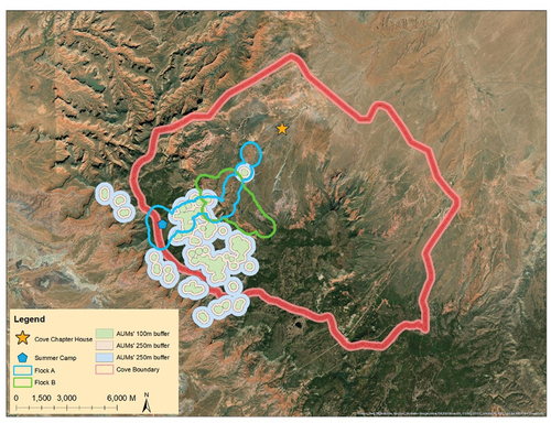
Figure 6. Daily exposure of flock A and flock B.

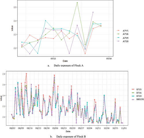
Figure 7. Geographic distribution of area associated with grazing, resting, and travelling for flock A and flock B.

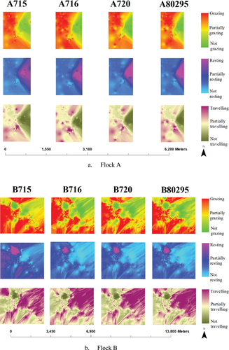
Figure 8. Daily exposure without considering behaviour patterns.

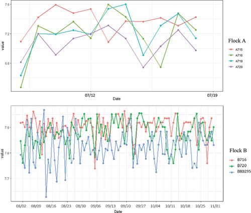
Figure 9. Daily exposure considering behaviour patterns but without probability/uncertainty.

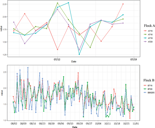
Figure 10. Points before and after the data preprocessing. (Note: Base map is excluded to protect livestock owner’s privacy).

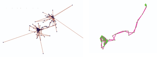
To protect livestock owners’ privacy, locational information of the livestock is presented with a 500-m buffer (Figure 5). Flock A spent most time in two places, the livestock corral downstream in the lower reaches of the watershed and a summertime grazing area higher in the watershed. They were kept inside the corral before July 8th, and then were held in the summer camp until July 19th. Generally, the flock only spent one or two hours in proximity to AUMs while they were travelling from the downstream corral to summer camp.

For Flock B, most locations were far from AUMs. A few paths intersected with 250 m/500 m buffers of the AUMs. In fact, only 0.44% of the data points were within 500 m of an AUM and only 0.03% of the points were within 250 m. As the distance from AUMs increases from 0 m to 100 m, elevated concentrations of toxic metals (e.g. radon, uranium, lead, etc.) in the soil and the atmosphere decrease significantly and eventually reach background levels as distance increases (Bunzl et al. 1994; Xie et al. 2014). Therefore, the 100 m buffer to AUMs is considered to be relatively high-risk; a 100 m to 250 m buffer is considered to be relatively medium-risk, and a 250 m to 500 m buffer is relatively low-risk.

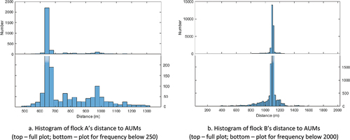
For livestock in Flock A, distance to AUMs varied from 486 to 1321 m and the average distance was 707 m. For livestock in Flock B, distance to AUMs varied from 125 to 1930 m and the average distance was 1086-m. Appendix Figure 11 displays a histogram of the livestock’s distances to AUMs. In general, most of the GPS points were in the area 500 m away from AUMs, where previous investigations indicated lower concentration of metals in soil and air (Bunzl et al. 1994; Xie et al. 2014).

Figure 11. Histograms of livestock distance to AUMs.

The daily cumulative exposure potential values for individual animals in Flock A are shown in Figure 6, ranging between 2.1 and 2.6. A higher value means that the livestock has a relatively higher exposure potential to waste from AUMs. The exposure values of the three individual livestock A715, A716 and A719 increased slightly from July 8th to July 13th, while exposure of another individual livestock A719 decreased first from July 8th to July 10th then increased to its highest value on July 11th. Two of the target livestock – A716 and A720 – had an increase from July 14th to July 15th. Estimated exposure of all four livestock decreased to their lowest on July 16th and increased again thereafter. An analysis of variance (ANOVA) test suggests no significant difference in daily exposure potential value for livestock in Flock A (p-value = 0.79 when July 19 was included, p-value = 0.82 when July 19 was excluded). The daily cumulative exposure potential results of Flock B are shown in Figure 6. For one animal (B715), the cumulative exposure potential could not be calculated for six days due to insufficient points after filtering. In terms of temporal pattern, Flock B had a higher exposure in August and mid-September, with exposure values higher than 2.5. Lower exposure values occur in October with values lower than 2. In general, the cumulative exposure potential decreased from August to October and followed a similar trend. An ANOVA suggests no significant difference in daily exposure potential values for Flock B (p-vale = 0.68).

After the fuzzy logic analysis, each GPS point was assigned three variables, each representing the fuzzy membership of grazing, resting, and travelling (Appendix Table 7 gives a sample result). Based on these three fuzzy memberships, a kriging interpolation method was used to generate a map showing areas where the flocks graze, rest, and travel (Figure 7).

Because Flock A was kept behind the fence by the livestock owner before July 8th, only GPS points around the summer camp were used to generate the map. For Flock A, all four livestock shared similar area when they were grazing, resting or travelling. Those four animals had relatively high probability of grazing in the north, west, and south portions of the study area. On the contrary, they only had relatively high resting probability to the west, and tend to have a high probability of travelling in the south.

After adding up the fuzzy membership of each behaviour, we derived the total membership of resting, grazing, and travelling for each animal, with which the frequency of each behaviour is calculated (Appendix Table 8 details the frequency of each individual’s behaviours). For each animal from Flock A, the resting frequency was around 63%, the grazing frequency was around 31%, and the travelling frequency was around 6%. Although the grazing area was larger than the resting area (Figure 7), the frequency of grazing was smaller than resting. The flock did not only rest when they were kept inside the fence from 8 pm to 8 am next morning, but also took some rest when they were at grazing time. Thus, it is reasonable that the resting frequency was larger than 50%.

Similar to Flock A, the four livestock from Flock B also shared similar area when they were grazing, resting or travelling (Figure 7). On the north-west side to the centroid point, they demonstrated a high probability of resting. On the west and south side, they demonstrated a high probability of grazing. These four animals were more likely to travel in the north-east of the study area.

For each animal from Flock B, the resting frequency was around 68%, the grazing frequency was around 28%, and the travelling frequency was around 4% (detailed frequency of Flock B’s behaviours is shown in Appendix Table 9). Similar to Flock A, the resting behaviour also had the highest frequency. The behaviour frequency was not significantly different among the animals from Flock B. However, the resting frequency increased by around 7% in October, and the frequency of grazing and travelling decreased as well. Because the weight of resting is the lowest, this helps explain the decreasing pattern of daily cumulative exposure potential in Figure 6.

When comparing daily exposure potential results between two flocks, Flock A (median value is 2.3) has an overall higher exposure potential when compared with Flock B (median value is 2.1). However, the frequency of resting of Flock A was smaller than that of Flock B, which could explain the results. Additionally, Flock A has lower variations in daily exposure than Flock B. These results, however, need to be corroborated by animal tissue and biomonitoring analysis results.

In order to demonstrate the robustness of the methods framework used in the research, two methods comparisons were conducted: a) comparison between the present method and those without considering behaviour patterns; and b) comparison between the present method and those without considering probability.

3.1. Comparison between the present method and those without considering behaviour patterns

As discussed in the methods section, the daily cumulative exposure potential is the weighted sum of the environmental contamination risk value of each possible behaviour pattern sequence (Table 2). However, if we do not account for behaviour patterns, the cumulative exposure potential would be the sum of the environmental contamination risk value along the travel route, which would be R1 + R2 + R3 (E1 in Figure 1). Results of the daily cumulative exposure potential for Flock A and B calculated with no behaviour pattern included is presented in Figure 8.

For Flock B, we only considered three animals due to missing data for one animal. After conversations with the livestock owner, we were aware that the flock tended to stay together when they were outside of livestock owner’s corral. As such, we can assume that all animals in the flock occupied the same general place when grazing, resting, or travelling. Thus, the environmental exposure potential value of those three individual livestock was likely to be similar based on GPS data. Also, they were likely to share similar behaviour patterns. A comparison of Figures 6, 8 indicates that results from the current method used in this study demonstrate more consistent patterns of environmental cumulative exposure potential within the same flock (p-value > 0.05 for both flocks, ANOVA test), while model results without behaviours included show significantly different patterns of environmental cumulative exposure potential (p-value of Flock B < 0.01, p-value of Flock A < 0.05, ANOVA test). Therefore, these results suggest that the present method framework results in more robust results that are closer to the expectation that livestock daily environmental cumulative exposure potential is similar within the flock (Figure 7).

3.2. Comparison between the present method and those without considering probability/uncertainty

In this case, we only considered the dominant behaviour defined as the behaviour with the highest probability among all behaviours. Through this experiment, we intended to verify the usefulness of applying fuzzy memberships in the calculation (Wan and Lin 2016; Zadeh 2008). Using only the dominant behaviour to calculate the daily cumulative exposure following the equation: $C_r={\sum }_l^n{W}_{i}R\left(t,l\right)$, where Wi represents the weight of the dominant behaviour i. As shown in Figure 1, the calculation of E₃ is based on this method. In this method, only one behaviour at each location is considered, rather than 27 combinations of behaviour sequences as shown in Table 2. Results from this method for Flock A and Flock B are presented in Figure 9.

As shown in Figure 9, the daily cumulative exposure potential demonstrates a similar pattern within flocks. However, this method was based on the principle that a dominant behaviour was given a probability of 100% – a crisp rather than fuzzy output for each location, which fails to consider uncertainties in behaviour classification. In fact, determining the dominant behaviour was challenging in some scenarios. For example, there were records whose fuzzy membership of resting and travelling were similarly low (e.g. row 8 in Appendix Table 7). There were also circumstances when the other behaviours were not small enough to be ignored even though one behaviour probability was the highest (e.g. row 7 in Appendix Table 7).

The statistical comparison between the current method and those without considering probability/uncertainty revealed that daily cumulative exposure potential estimated without probability/uncertainty for individual livestock within the same flock was more likely to be significantly different from each other than the current method, based on the p-values (Appendix Table 10). This could further indicate that the exposure results generated from the current method are closer to reality.

A closer comparison among Figures 6, 9 veals that the daily cumulative environmental exposure potential among the Flock B had higher variance if probability of all behaviours were considered. For example, the environmental exposure potential for B716, B720 and B80295 on August 12th are 2.28, 2.06 and 2.53 in Figure 9 (without probability/uncertainty), respectively. However, when we considered behaviours, the corresponding values are 2.57, 2.51 and 2.56 (Figure 6). From 12 selected points on that day, we found that for 5 1-h periods, at least one animal’s behaviour could not be conclusively determined by the highest value of three fuzzy memberships because their differences were not significant enough to justify the omission of other behaviours. For example, from 9:00 to 10:00 (second row in Table 3), the fuzzy membership of grazing of these three animals was around 0.5 which could not be simply overlooked even though the travelling probability was higher. In such case, the potential of other behaviours should not be overlooked.

Table 3. Fuzzy membership of flock B on August 12th.

B716					B720				B80295
time	FM_G		FM_R	FM_T	time	FM_G	FM_R	FM_T	time	FM_G	FM_R	FM_T
8:20	0.30		1.00	0.00	8:20	0.30	1.00	0.00	8:20	0.30	1.00	0.00
9:40	0.51		0.09	0.79	9:40	0.45	0.06	0.85	9:41	0.56	0.11	0.74
10:20	1.00		0.30	0.30	10:20	0.97	0.29	0.33	10:20	0.97	0.29	0.33
11:20	1.00		0.30	0.30	11:20	1.00	0.30	0.30	11:20	1.00	0.30	0.30
12:20	1.00		0.30	0.30	12:21	1.00	0.30	0.30	12:20	1.00	0.30	0.30
13:41	0.74		0.19	0.56	13:20	0.99	0.29	0.31	13:20	0.98	0.29	0.32
14:20	0.02		0.34	0.28	15:00	0.24	0.86	0.06	14:21	0.01	0.32	0.29
15:20	0.30		1.00	0.00	15:20	0.30	1.00	0.00	15:20	0.30	1.00	0.00
16:20	0.30		1.00	0.00	16:20	0.30	1.00	0.00	16:20	0.30	1.00	0.00
17:20	0.30		1.00	0.00	17:20	0.30	1.00	0.00	17:20	0.30	1.00	0.00
18:20	0.59		0.12	0.71	18:20	0.65	0.15	0.65	18:20	0.55	0.11	0.75
19:20	0.53		0.13	0.71	19:20	0.48	0.11	0.76	19:20	0.52	0.11	0.76

Notes: 1. FM_G – fuzzy membership of grazing; FM_R – fuzzy membership of resting; FM_T – fuzzy membership of travelling. 2. Two points of B716 were selected on 9:40 and 13:41because points on 9:20 and 13:20 were missing.

Table 4 lists the frequency of how many behaviour probabilities are 0.5 larger than the rest. For two flocks, around 67% of GPS points had a resting probability 0.5 larger than that of grazing and travelling. Around 17% of points had grazing probability 0.5 larger than the other two. Only about 1% of points travelling behaviour had higher fuzzy membership. In total, there were 85.7% points, among which the fuzzy membership of one behaviour pattern was 0.5 larger than the other two behaviours. We still had 14.3% points with undetermined dominant behaviour. We conclude that although the method considering probability/uncertainty was less computationally intensive, the proposed method is extensible to more real-world scenarios, especially when a dominant behaviour cannot be determined.

Table 4. Frequency of dominant behaviour.

	A715	A716	A719	A720	B716	B720	B80295	All individual
Resting	47.68%	47.66%	49.73%	46.96%	72.23%	71.47%	67.53%	67.27%
Grazing	25.34%	28.93%	26.78%	25.97%	14.00%	14.79%	17.17%	16.91%
Travelling	0.54%	0.55%	0.55%	0.55%	1.38%	1.64%	2.10%	1.52%
Total	73.57%	77.13%	77.05%	73.48%	87.61%	87.91%	86.81%	85.70%

1) The dominant behaviour was determined with the following condition: grazing: FM_G > (FM_R + 0.5 and FM_T + 0.5) resting: FM_R > (FM_G + 0.5 and FM_T + 0.5) travelling: FM_T > (FM_G + 0.5 and FM_R + 0.5). 2) FM_G – fuzzy membership of grazing; FM_R – fuzzy membership of resting; FM_T – fuzzy membership of travelling

4. Discussion

This research is situated at the intersection of time geography, GIS/GPS methods, parallel computing, and environmental exposure assessments. We examined the geospatial and temporal behaviour patterns of domesticated livestock and modelled potential cumulative exposure to AUM waste at the individual animal level with corresponding uncertainty. A total of eight animals (four sheep and four goats) were fitted with GPS collars. Due to the terrain and canopy effects, some GPS data points were considered invalid. We intended to quantify the cumulative exposure risk as a sum of the product of probability of classified livestock behaviour and environmental contamination for every GPS point location. However, the GPS data for one livestock animal was too large for a single linear calculation, which would generate one single number representing the total cumulative exposure potential for that animal during the whole recording period. Thus, this research employed parallel computing to calculate daily cumulative exposure potential to AUMs and AUM waste, which significantly lowered the number of GPS points for the aforementioned calculation. Yet, the calculation task was still impossible for a personal computer to complete. To overcome the N-P problem, we shifted our research focus to the time window from 8:00 AM to 8:00 PM when the animals might be grazing, and we selected only one GPS point every hour to represent the behaviour pattern for that hour. Fuzzy rules were then applied to categorize the behaviour patterns of animals, that is, grazing or resting, and the possibilities of corresponding behaviours.

According to the results, the daily cumulative exposure potential of Flock A ranges from 2.1 to 2.6, the average value was approximately 2.3. Cumulative exposure, in this case, is dimensionless. However, there is not enough evidence to conclude that there are significant differences in the potential exposure among the four individuals. For Flock B, the daily cumulative exposure potential varied from 1.8 to 2.8. The average value was approximately 2.1. Not only do behaviour patterns affect an animal’s exposure potential, but the environmental contamination value at each GPS location also impacts the results. We adopted an environmental exposure potential model of this study area from a previous study (Kurttio et al. 2006). However, grazing behaviours certainly have a higher impact on the final results since two exposure routes were considered and higher weight was assigned compared to other behaviours. These results similarly need to be corroborated by animal tissue and biomonitoring analysis results.

The cumulative exposure potential estimates proposed in this paper were built on widely adopted human exposure risk assessment models. There is little research that applies similar approaches on livestock exposure estimates. We adapted previous methods used for human environmental exposure assessment to livestock study and enhanced the methods by introducing a fuzzy logic-based behaviour classification to mitigate uncertainties. A comparison of the proposed methods with previous approaches on probability-based risk assessments reveal that our approach is more robust for individual-level livestock exposure potential modelling using GPS data. Other methods that do not account for behaviours or behaviour probability/uncertainties resulted in significantly different daily cumulative environmental exposure potential, which does not fit with the assumption that these animals tended to stay in one group. Additionally, another contribution of this study is that it is a GIS-based study informed largely by Native American culture and community involvement.

5. Limitations of the research

Due to the uncontrollable environmental influences, the GPS device performance, recent computing abilities, etc., this research has several limitations.

First, this research used a filtering strategy to solve the N-P problem, which was discussed in the methodology section. However, the filtering method employed could potentially misrepresent all GPS data during a given hour. Additionally, the recording interval of the GPS devices were set to be 20 minutes, which meant that we only had 3 points at most for every hour. However, when all 3 GPS records from one hour period were invalid, we used the previous hour or the next hour to search for a point to represent the current hour (less than 5% of data were under this scenario). Another possible solution offered here is that in the deficiency of high-performance computing resources, one could significantly decrease the number of selected GPS points by only including represented points to increase the computational efficiency.

The second limitation is related to animal behaviour patterns. We initially intended to use four behaviour patterns – grazing, resting, travelling, and drinking – to calculate the cumulative exposure potential, but this would raise the calculation up to 4ⁿ times (n is the points number we selected). Oral exposure would also be separated into two subgroups – drinking and eating. To decrease the burden of the computing and cover as much time in a day as possible, we used the three most representative behaviour patterns of livestock – grazing, resting, and travelling. Additionally, we only used two factors for fuzzy membership behaviour classification because our classification was partially informed by livestock owners. For grazing behaviour classification, the general grazing area was known. The general pattern of travelling and resting were also known. Therefore, factors such as terrain, sunlight, and vegetation were less important or have little relevance in the classification. Future studies might consider integrating accelerometer or activity sensor to better predict animal behaviours (Rodriguez-Baena et al. 2020; Zehner et al. 2017). Moreover, we did not conduct a formal assessment of the accuracy of behaviour pattern classification because ground truthing at a fine spatial-temporal scale was not feasible. On the other hand, this study employs fuzzy logic, which has an advantage of addressing classification uncertainties through generating probabilities. We worked together with livestock owners to review the general patterns of behaviours after classification, which agreed with their understanding. In fact, information and knowledge about livestock behaviours through communication with livestock owners were used in the classification process. Nevertheless, future studies should collect point to point ground truthing data using different technologies (e.g. GoPro camera) to verify results.

Third, this research set weights of grazing, resting and travelling as 2:1:2, respectively, when estimating the cumulative exposure potential based on assumptions that the oral exposure and respiratory exposure were equally accumulated inside livestock’s body and the respiratory exposure while travelling is twice that of grazing and resting. More biological research is needed to verify and determine the relative importance of exposure between grazing and resting.

Fourth, the current study does not have a control set of livestock from uncontaminated places for the whole study duration. Therefore, it was not possible to compare our results against that from any control flock. Results from this study could have been influenced by prior long-term exposure as well as due to a lack of data prior to collaring.

Lastly, results from this study will need to be verified by animal tissue and organ sample analysis. As a collaborative research project, results from this study will be compared with levels of heavy metals detected in tissue and organs of individual livestock analysed by our research partners. Nevertheless, this geospatial research provides a useful and reliable methodological framework for livestock exposure assessments in geographic areas with environmental contamination to understand and address environmental health questions.

6. Implication for future study

This is the first study combining time geography, GIS, and behaviour pattern classification to create a new workflow to estimate livestock cumulative exposure potential. Results from this study can be further used to guide livestock owners to optimize grazing or pasturing to reduce potential exposure. The workflow presented here could potentially be adapted or extended to other areas of Navajo Nation and other geographic regions with multiple types of environmental contamination. This study has potential to inform research about animal exposure to the environment.

Disclosure statement

No potential conflict of interest was reported by the author(s).

Additional information

Funding

This work was supported by No. V-99T54301-2 awarded by the U.S. Environmental Protection Agency to Dine’ College. Additional funding in support of this project by NIH (1P50ES026089) & USEPA (#83615701), NIMHD P50 MD015706, and NIEHS P42 ES025589.

APPENDIX

Table 5. GPS data sample.

GMT Time	Lat	Lon	Alt (metre)	Duration (second)	Temp (°C)	DOP	Satellites
6/24/2019 4:42:12 PM	0	0	0	2	24.5	0	0
6/24/2019 5:01:10 PM	0	0	0	70	29.5	0	0
6/24/2019 5:20:27 PM	35.09131	−106.617	1556.96	41	27	1.6	5
6/24/2019 5:40:28 PM	35.09127	−106.617	1542.07	27	25.5	1.6	5

Notes. GMT – Greenwich Mean Time; Lat – Latitude; Lon – Longitude; Alt – Altitude; Duration – the time it takes to connect to satellite; Temp – temperature; DOP – dilution of precision; Satellites – number of connected satellites

Table 6. Basic information of datasets.

Livestock	Total Points Collected	Duration = 70s	Number of Satellites < 4	Altitude < 800 m	Number of Valid Points
A715	2122	147 (6.93%)	81 (3.82%)	70 (3.30%)	1961 (92.41%)
A716	2091	181 (8.66%)	86 (4.11%)	80 (3.83%)	1902 (90.96%)
A719	2137	150 (7.02%)	73 (3.42%)	66 (3.09%)	1978 (92.56%)
A720	2098	204 (9.72%)	100 (4.77%)	86 (4.10%)	1878 (85.44%)
B715	7572	1201 (15.86%)	592 (7.82%)	610 (8.06%)	6214 (82.06%)
B716	8143	330 (4.05%)	116 (1.42%)	120 (1.47%)	7767 (95.38%)
B720	8085	453 (5.60%)	189 (2.34%)	187 (2.31%)	7561 (93.52%)
B80295	7957	650 (8.17%)	297 (3.73%)	279 (3.51%)	7204 (90.54%)

Table 7. Sample result of fuzzy logic for behaviour classification.

FID	Local Time	FM_G	FM_R	FM_T
0	7/25/2019 15:40	0.3	1	0
1	7/25/2019 16:00	0.3	1	0
2	7/25/2019 16:21	0.3	1	0
3	7/25/2019 16:40	0.3	1	0
4	7/25/2019 17:00	0.3	1	0
5	7/25/2019 18:20	0.96591	0.329212	0.290145
6	7/25/2019 18:40	0.907084	0.260179	0.392916
7	7/25/2019 19:00	0.855618	0.238122	0.444382
8	7/25/2019 19:20	0.025429	0.359334	0.274571
…	…	…	…	…
Notes. FM_G – fuzzy membership of grazing; FM_R – fuzzy membership of resting; FM_T – fuzzy membership of travelling;

Table 8. Frequency of resting, grazing, and travelling of flock A.

	A715	A716	A719	A720	All individual
Resting	63.31%	62.85%	63.08%	62.90%	63.04%
Grazing	30.51%	31.00%	30.61%	30.79%	30.72%
Travelling	6.18%	6.15%	6.32%	6.32%	6.24%

Table 9. Frequency of resting, grazing, and travelling of flock B.

		B715	B716	B720	B80295	All individual
Resting	All Months	67.06%	68.52%	68.47%	67.76%	68.00%
Grazing		28.18%	27.28%	27.32%	27.71%	27.60%
Travelling		4.76%	4.20%	4.20%	4.53%	4.40%
Resting	Aug	64.61%	65.81%	66.37%	64.93%	65.47%
Grazing		28.99%	28.27%	27.94%	28.72%	28.45%
Travelling		6.40%	5.92%	5.70%	6.35%	6.07%
Resting	Sep	64.44%	66.62%	65.79%	65.32%	65.59%
Grazing		30.12%	28.70%	29.18%	29.49%	29.34%
Travelling		5.44%	4.68%	5.03%	5.19%	5.07%
Resting	Oct	72.39%	73.15%	73.22%	73.10%	72.99%
Grazing		25.29%	24.87%	24.88%	24.90%	24.97%
Travelling		2.32%	1.98%	1.90%	2.00%	2.03%

Table 10. T-test of daily cumulative exposure potential of flock B comparison of the current method with those not considering probability/uncertainty.

P-value	B716		B720		B80295
	Current method	without probability/uncertainty	Current method	without probability/uncertainty	Current method	without probability/uncertainty
B716			0.559	$9.7\times {10}^{-4}$	0.044	$6.2\times {10}^{-5}$
B720	0.559	$9.7\times {10}^{-4}$			0.145	$0.175$
B80295	0.044	$6.2\times {10}^{-5}$	0.145	$0.175$

References

- Allan, B. M., J. P. Arnould, J. K. Martin, and E. G. Ritchie. 2013. “A cost-effective and Informative Method of GPS Tracking Wildlife.” Wildlife Research 40 (5): 345–348. doi:10.1071/WR13069.
- Anke, M., O. Seeber, R. Müller, U. Schäfer, and J. Zerull. 2009. “Uranium Transfer in the Food Chain from Soil to Plants, Animals and Man.” Geochemistry 69: 75–90. doi:10.1016/j.chemer.2007.12.001.
- Augustine, D. J., and J. D. Derner. 2013. “Assessing Herbivore Foraging Behavior with GPS Collars in a Semiarid Grassland.” Sensors 13 (3): 3711–3723. doi:10.3390/s130303711.
- Barbone, F., M. Bovenzi, F. Cavallieri, and G. Stanta. 1995. “Air Pollution and Lung Cancer in Trieste, Italy.” American Journal of Epidemiology 141 (12): 1161–1169. doi:10.1093/oxfordjournals.aje.a117389.
- Bolt, A. M., S. Medina, F. T. Lauer, H. Xu, A. M. Ali, K. J. Liu, S. W. Burchiel, and M. F. Khan. 2018. “Minimal Uranium Accumulation in Lymphoid Tissues following an Oral 60-day Uranyl Acetate Exposure in Male and Female C57BL/6J Mice.” Plos one 13 (10): e0205211. doi:10.1371/journal.pone.0205211.
- Brown, J. D. 2004. “Knowledge, Uncertainty and Physical Geography: Towards the Development of Methodologies for Questioning Belief.” Transactions of the Institute of British Geographers 29 (3): 367–381. doi:10.1111/j.0020-2754.2004.00342.x.
- Brugge, D., and R. Goble. 2002. “The History of Uranium Mining and the Navajo People.” American Journal of Public Health 92 (9): 1410–1419. doi:10.2105/AJPH.92.9.1410.
- Brugge, D., J. L. deLemos, and B. Oldmixon. 2005. “Exposure Pathways and Health Effects Associated with Chemical and Radiological Toxicity of Natural Uranium: A Review.” Reviews on Environmental Health 20 (3): 177–194. doi:10.1515/REVEH.2005.20.3.177.
- Bunzl, K., R. Kretner, M. Szeles, and R. Winkler. 1994. “Transect Survey of 238U, 228Ra, 226Ra, 210Pb, 137Cs and 40K in an Agricultural Soil near an Exhaust Ventilating Shaft of a Uranium Mine.” Science of the Total Environment 149 (3): 225–232. doi:10.1016/0048-9697(94)90181-3.
- Craft, E. S., A. W. Abu-Qare, M. M. Flaherty, M. C. Garofolo, H. L. Rincavage, and M. B. Abou-Donia. 2004. “Depleted and Natural Uranium: Chemistry and Toxicological Effects.” Journal of Toxicology and Environmental Health, Part B 7 (4): 297–317. doi:10.1080/10937400490452714.
- Eichstaedt, P. H. 1994. If You Poison Us: Uranium and Native Americans. 1st. New Mexico, USA: Red Crane Books.
- Fettus, G. H., and M. G. McKinzie. 2012. Nuclear Fuel’s Dirty Beginnings. https://www.nrdc.org/sites/default/files/uranium-mining-report.pdf
- Fijałkowska–Lichwa, L. 2016. “Extremely High Radon Activity Concentration in Two Adits of the Abandoned Uranium Mine ‘Podgórze’in Kowary (Sudety Mts., Poland).” Journal of Environmental Radioactivity 165: 13–23. doi:10.1016/j.jenvrad.2016.08.016.
- Fortnow, L. 2009. “The Status of the P versus NP Problem.” Communications of the ACM 52 (9): 78–86. doi:10.1145/1562164.1562186.
- Gong, G., S. Mattevada, and S. E. O’Bryant. 2014. “Comparison of the Accuracy of Kriging and IDW Interpolations in Estimating Groundwater Arsenic Concentrations in Texas.” Environmental Research 130: 59–69. doi:10.1016/j.envres.2013.12.005.
- Gottlieb, L. S., and L. A. Husen. 1982. “Lung Cancer among Navajo Uranium Miners.” Chest 81 (4): 449–452. doi:10.1378/chest.81.4.449.
- Gramss, G., and K.-D. Voigt. 2014. “Forage and Rangeland Plants from Uranium Mine Soils: Long-term Hazard to Herbivores and Livestock?” Environmental Geochemistry and Health 36 (3): 441–452. doi:10.1007/s10653-013-9572-5.
- Hägerstraand, T. 1970. “What about People in Regional Science?” Papers in Regional Science 24 (1): 7–24. doi:10.1111/j.1435-5597.1970.tb01464.x.
- Handcock, R. N., D. L. Swain, G. J. Bishop-Hurley, K. P. Patison, T. Wark, P. Valencia, C. J. O’Neill, and C. O’Neill. 2009. “Monitoring Animal Behaviour and Environmental Interactions Using Wireless Sensor Networks, GPS Collars and Satellite Remote Sensing.” Sensors 9 (5): 3586–3603. doi:10.3390/s90503586.
- Harrison, R. M., P. L. Leung, L. Somervaille, R. Smith, and E. Gilman. 1999. “Analysis of Incidence of Childhood Cancer in the West Midlands of the United Kingdom in Relation to Proximity to Main Roads and Petrol Stations.” Occupational and Environmental Medicine 56 (11): 774–780. doi:10.1136/oem.56.11.774.
- Holaday, D. A. 1969. “History of the Exposure of Miners to Radon.” Health Physics 16 (5): 547–552. doi:10.1097/00004032-196905000-00001.
- Hoover, J., M. Gonzales, C. Shuey, Y. Barney, and J. Lewis. 2017. “Elevated Arsenic and Uranium Concentrations in Unregulated Water Sources on the Navajo Nation, USA.” Exposure and Health 9 (2): 113–124. doi:10.1007/s12403-016-0226-6.
- Hoover, J. H., E. Erdei, D. Begay, M. Gonzales, J. M. Jarrett, P. Y. Cheng, and J. Lewis; NBCS Study Team. 2020. “Exposure to Uranium and co-occurring Metals among Pregnant Navajo Women.” Environmental Research 190: 109943. doi:10.1016/j.envres.2020.109943.
- Hornung, R. W., and T. J. Meinhardt. 1987. “Quantitative Risk Assessment of Lung Cancer in US Uranium Miners.” Health Physics 52 (4): 417–430. doi:10.1097/00004032-198704000-00002.
- Jenelius, E., T. Petersen, and L. G. Mattsson. 2006. “Importance and Exposure in Road Network Vulnerability Analysis.” Transportation Research Part A: Policy and Practice 40 (7): 537–560.
- Kim, H. M., and M. P. Kwan. 2003. “Space-time Accessibility Measures: A Geocomputational Algorithm with A Focus on the Feasible Opportunity Set and Possible Activity Duration.” Journal of Geographical Systems 5 (1): 71–91. doi:10.1007/s101090300104.
- Kurttio, P., A. Harmoinen, H. Saha, L. Salonen, Z. Karpas, H. Komulainen, and A. Auvinen. 2006. “Kidney Toxicity of Ingested Uranium from Drinking Water.” American Journal of Kidney Diseases 47 (6): 972–982. doi:10.1053/j.ajkd.2006.03.002.
- Kwan, M. P. 1998. “Space‐time and Integral Measures of Individual Accessibility: A Comparative Analysis Using a Point‐based Framework.” Geographical Analysis 30 (3): 191–216. doi:10.1111/j.1538-4632.1998.tb00396.x.
- Kwan, M. P., and T. Schwanen. 2018. “Context and Uncertainty in Geography and GIScience: Advances in Theory, Method, and Practice.” Annals of the American Association of Geographers 108 (6): 1473–1475. doi:10.1080/24694452.2018.1457910.
- Leelasakultum, K., and N. T. Kim Oanh. 2017. “Mapping Exposure to Particulate Pollution during Severe Haze Episode Using Improved MODIS AOT‐PM10 Regression Model with Synoptic Meteorology Classification.” GeoHealth 1 (4): 165–179. doi:10.1002/2017GH000059.
- Lin, Y., J. Hoover, D. Beene, E. Erdei, and Z. Liu. 2020. “Environmental Risk Mapping of Potential Abandoned Uranium Mine Contamination on the Navajo Nation, USA, Using a GIS-based multi-criteria Decision Analysis Approach.” Environmental Science and Pollution Research International 27 (24): 30542–30557. doi:10.1007/s11356-020-09257-3.
- Lu, Y., and T. B. Fang. 2015. “Examining Personal Air Pollution Exposure, Intake, and Health Danger Zone Using Time Geography and 3D Geovisualization.” ISPRS International Journal of Geo-Information 4 (1): 32–46. doi:10.3390/ijgi4010032.
- Medina, S., F. T. Lauer, E. F. Castillo, A. M. Bolt, A. M. S. Ali, K. J. Liu, and S. W. Burchiel. 2020. “Exposures to Uranium and Arsenic Alter Intraepithelial and Innate Immune Cells in the Small Intestine of Male and Female Mice.” Toxicology and Applied Pharmacology 403: 115155. doi:10.1016/j.taap.2020.115155.
- Meinrath, A., P. Schneider, and G. Meinrath. 2003. “Uranium Ores and Depleted Uranium in the Environment, with a Reference to Uranium in the Biosphere from the Erzgebirge/Sachsen, Germany.” Journal of Environmental Radioactivity 64 (2–3): 175–193. doi:10.1016/S0265-931X(02)00048-6.
- Miller, H. J. 1991. “Modelling Accessibility Using space-time Prism Concepts within Geographical Information Systems.” International Journal of Geographical Information Systems 5 (3): 287–301. doi:10.1080/02693799108927856.
- Moolgavkar, S. H. 2000. “Air Pollution and Daily Mortality in Three US Counties.” Environmental Health Perspectives 108 (8): 777–784. doi:10.1289/ehp.00108777.
- Mudd, G. M. 2008. “Radon Releases from Australian Uranium Mining and Milling Projects: Assessing the UNSCEAR Approach.” Journal of Environmental Radioactivity 99 (2): 288–315. doi:10.1016/j.jenvrad.2007.08.001.
- Mulloy, K. B., D. S. James, K. Mohs, and M. Kornfeld. 2001. “Lung Cancer in a Nonsmoking Underground Uranium Miner.” Environmental Health Perspectives 109 (3): 305–309. doi:10.1289/ehp.01109305.
- Oren, T. I., and N. Ghasem-Aghaee (2003, July). Personality Representation Processable in Fuzzy Logic for Human Behavior Simulation. In Summer Computer Simulation Conference, Montreal, PQ, Canada (pp. 11–18). Society for Computer Simulation International; 1998.
- Raubal, M., H. J. Miller, and S. Bridwell. 2004. “User‐centred Time Geography for Location‐based Services.” Geografiska annaler. Series B, Human geography 86 (4): 245–265. doi:10.1111/j.0435-3684.2004.00166.x.
- Rife, J., and S. M. Rock 2001, . Visual Tracking of Jellyfish in Situ. In Proceedings 2001 International Conference on Image Processing (Cat), Thessaloniki, Greece (Vol. 1, pp. 289–292). IEEE.
- Rodriguez-Baena, D. S., F. A. Gomez-Vela, M. García-Torres, F. Divina, C. D. Barranco, N. Daz-Diaz, G. Montalvo, and G. Montalvo. 2020. “Identifying Livestock Behavior Patterns Based on Accelerometer Dataset.” Journal of Computational Science 41: 101076. doi:10.1016/j.jocs.2020.101076.
- Ryan, P. H., and G. K. LeMasters. 2007. “A Review of land-use Regression Models for Characterizing Intraurban Air Pollution Exposure.” Inhalation Toxicology 19 (sup1): 127–133. doi:10.1080/08958370701495998.
- Samet, J. M., D. M. Kutvirt, R. J. Waxweiler, and C. R. Key. 1984. “Uranium Mining and Lung Cancer in Navajo Men.” New England Journal of Medicine 310 (23): 1481–1484. doi:10.1056/NEJM198406073102301.
- Tannenbaum, A., H. Silverstone, and J. Koziol. 1948. Tracer Studies on the Distribution and Excretion of Uranium in Mice, Rats, and Dogs. Oak Ridge, Tennessee, USA: US Atomic Energy Commission, Technical Information Division.
- Tobler, W. R. 1970. “A Computer Movie Simulating Urban Growth in the Detroit Region.” Economic Geography 46 (sup1): 234–240. doi:10.2307/143141.
- Turner, L. W., M. C. Udal, B. T. Larson, and S. A. Shearer. 2000. “Monitoring Cattle Behavior and Pasture Use with GPS and GIS.” Canadian Journal of Animal Science 80 (3): 405–413. doi:10.4141/A99-093.
- Vaupotić, J. 2001. “Radon and gamma-radiation Measurements in Schools on the Territory of the Abandoned Uranium Mine “Žirovski Vrhl”.” Journal of Radioanalytical and Nuclear Chemistry 247 (2): 291–295. doi:10.1023/A:1006741215350.
- Wan, N., and G. Lin. 2016. “Classifying Human Activity Patterns from Smartphone Collected GPS Data: A Fuzzy Classification and Aggregation Approach.” Transactions in GIS 20 (6): 869–886. doi:10.1111/tgis.12181.
- Wang, J., M. P. Kwan, and Y. Chai. 2018. “An Innovative context-based crystal-growth Activity Space Method for Environmental Exposure Assessment: A Study Using GIS and GPS Trajectory Data Collected in Chicago.” International Journal of Environmental Research and Public Health 15 (4): 703. doi:10.3390/ijerph15040703.
- Weber, J. 2003. “Individual Accessibility and Distance from Major Employment Centers: An Examination Using space-time Measures.” Journal of Geographical Systems 5 (1): 51–70. doi:10.1007/s101090300103.
- Weston Solutions, Inc. (2014) Mesa I, Mines 10-15-Abandoned Uranium Mine Site Reassessment Report. (EPA ID No.: NND983466772). https://www.epa.gov/sites/production/files/2016-10/documents/mesa_i_mines_final_reassessment_report_2014-01.pdf
- Xie, D., H. Wang, K. J. Kearfott, Z. Liu, and S. Mo. 2014. “Radon Dispersion Modeling and Dose Assessment for Uranium Mine Ventilation Shaft Exhausts under Neutral Atmospheric Stability.” Journal of Environmental Radioactivity 129: 57–62. doi:10.1016/j.jenvrad.2013.12.003.
- Yazzie, S. A., S. Davis, N. Seixas, and M. G. Yost. 2020. “Assessing the Impact of Housing Features and Environmental Factors on Home Indoor Radon Concentration Levels on the Navajo Nation.” International Journal of Environmental Research and Public Health 17 (8): 2813. doi:10.3390/ijerph17082813.
- Zadeh, L. A. 1965. “Fuzzy Sets.” Information and Control 8 (3): 338–353. doi:10.1016/S0019-9958(65)90241-X.
- Zadeh, L. A. 2008. “Is There a Need for Fuzzy Logic?” Information Sciences 178 (13): 2751–2779. doi:10.1016/j.ins.2008.02.012.
- Zamora, M. L., B. L. Tracy, J. M. Zielinski, D. P. Meyerhof, and M. A. Moss. 1998. “Chronic Ingestion of Uranium in Drinking Water: A Study of Kidney Bioeffects in Humans.” Toxicological Sciences 43 (1): 68–77. doi:10.1093/toxsci/43.1.68.
- Zehner, N., C. Umstätter, J. J. Niederhauser, and M. Schick. 2017. “System Specification and Validation of a Noseband Pressure Sensor for Measurement of Ruminating and Eating Behavior in stable-fed Cows.” Computers and Electronics in Agriculture 136: 31–41. doi:10.1016/j.compag.2017.02.021.
- Zhan, Y., Y. Luo, X. Deng, K. Zhang, M. Zhang, M. L. Grieneisen, and B. Di. 2018. “Satellite-based Estimates of Daily NO2 Exposure in China Using Hybrid Random Forest and Spatiotemporal Kriging Model.” Environmental Science & Technology 52 (7): 4180–4189. doi:10.1021/acs.est.7b05669.