Production of orthophoto map using mobile photogrammetry and comparative assessment of cost and accuracy with satellite imagery for corridor mapping: a case study in Manesar, Haryana, India

ABSTRACT

The study aims to find a low-cost alternate technology to get imagery, using mobile platform, and produce digital orthophoto for corridor mapping, with a higher degree of accuracy and which can reduce the lag time of acquisition of data. The present study uses digital single-lens reflex cameras, mounted on a mobile vehicle, and acquisition of data in the video format rather than still photographs, as traditionally used in mobile mapping systems. The videos are used to create a set of images and orthophotos. A widespread ground control points were recorded in the study area, using the global navigation satellite system receiver, which measured the control points in real-time kinematic mode. Generation of digital orthophoto has been completed using the captured mobile imagery and ground control point. Furthermore, procurement of satellite imagery and aerial triangulation using ground control points have been done. While comparing the planimetric accuracy of orthophoto against satellite imagery using the ground control points, the achieved root mean square error value of produced orthophoto is 0.171 m in X axis and 0.205 m in Y axis. However, for Cartosat -1 satellite imagery, the RMSE value for X is 1.22 m and for Y is 1.98 m. This research proposes the alternate low-cost mobile mapping method to capture the imagery for orthophoto production. The cost of orthophoto production from mobile image was found 77% cheaper than the orthophoto cost from fresh/latest satellite imagery procurement, while the overall production was 70% cost-effective than the orthophoto maps made from archived imagery.

KEYWORDS:

• Mobile mapping
• corridor mapping orthophoto
• GNSS
• RTK (real-time kinematics)
• stereo satellite images
• panoramic imagery
• RMSE (root mean square Error)

1. Introduction

Digital orthophoto maps produced using satellite imagery are preferred over classical maps due to economic considerations (Aparajithan, Donald, and Christophersona 2012). Advancement in technology for data acquisition, as an input for geographical information system (GIS), remote sensing and digital photogrammetry (Altmana et al., 2017) have rapidly enhanced in recent years. Using unmanned aerial vehicles (UAVs) and aerial and satellite imageries, the most recent spatial information can be supplied for mapping services (Ferrer-González et al. 2020; Nikolakopoulos et al. 2016; Lin et al. 2021; Pech et al. 2013). For larger areas, the digital orthophoto maps produced using aerial and satellite imagery can supply fast and economical map for production in mapping industries (Alan et al. 2004). For small mapping projects, such as road corridor, the needs of digital orthophoto (Joachim, 1996) have gained widespread recognition and application in precise mapping of road marks, limits, curbs (Zhao and Yuan, 2012), inventories, road surface modelling (Khoshelham, 2005), road quality analysis, itinerary computations and image-based localization for ground landmarks (Hervieu, Soheilian, and Bredif 2015; McElhinney et al. 2010; El-Halawany et al. 2011; Pu et al. 2011; Hervieu and Soheilian 2013a; Serna and Marcotegui 2013; Qu, Soheilian, and Paparoditis 2015). To optimize the cost of project, primary data acquisition using mobile mapping equipment (Bitenc et al., 2011) can provide a better solution for production of orthophoto of smaller area as compared to imagery from satellite and aerial photography (Vallet and Papelard 2015).

Mapping in recent years has undergone a paradigm shift with constant improvement in the airborne sensors and high-resolution satellite data (Christoph et al. 2013). The airborne sensors can achieve an accuracy (Dial, 2000) in a range of less than 5 cm. Satellite imageries of up to 30 cm ground sample distance (GSD) are commercially available for some areas of the United States and Europe. Unmanned aerial vehicles (UAVs), as part of mapping, also bring in high accuracy data with planimetric accuracies ranging from 2 to 3 cm on orthophotos (Yu et al. 2018) Recently, UAV photogrammetry has been identified as a popular, fast, and cost-effective solution for projects in complex terrain for orthophoto and digital surface models (DSMs; Ferrer-González et al. 2020). Orthophoto production using motion photogrammetry with photo data acquired by UAVs (Peter, 1999) was recently inducted (Kyriou et al. 2021) where digital orthophoto at 4 cm has been generated for the study of landslides.

As an alternate method, mobile sensors are also available to capture the light detection and ranging (LiDAR) data and are quite efficient and correct (Serna and Marcotegui 2013). Mobile mapping as a technology to capture panoramic imagery with enhanced accuracy has gained widespread acceptance in the past decade for corridor mapping. Its high-resolution camera captures photographs, while inbuilt global navigation satellite system (GNSS) and inertial measurement units (IMUs) ensure positional accuracy while getting data through a moving platform. The developed trajectory from the moving platform along with the navigation system allows direct georeferencing of the acquired data. However, getting data using the above technologies demands resources, statutory government permissions and high cost for execution.

Lately, many ways for creating orthophotos with a digital single-lens reflex (DSLR) camera have been proposed (Aparajithan, Donald, and Christophersona 2012; Birutė 2005; Qu, Soheilian, and Paparoditis 2015). The extraction of point clouds from terrestrial images (Jauregui and Jauregui, 2000) has been a significant subject of interest in the geospatial arena, with work on similar goals readily available in the literature. The generation of orthophotos utilizing the processing of calibrated or uncalibrated photographs is described in a variety of publications, along with strategies for obtaining positional accuracies. Comparing the accuracies of DSM built using aerial image, satellite imagery and LiDAR scanning data is a work reference available. In an urban context where the GNSS signal is not optimal, a comprehensive study has been given for the registration of mobile images as well as satellite imagery (Fanta-Jende et al. 2017). A detailed statistical examination of the accuracy of LiDAR point clouds obtained by a mobile mapping device and another method has been given (Toschi et al. 2015). Using aerial imagery and point cloud from a terrestrial laser scanner, a simpler method of large-scale orthophoto generation was developed (Fanta-Jende et al. 2017). This method entails the capture of aerial photographs as well as point cloud data, resulting in a more straightforward production method despite the high expense of data acquisition. There has been ortho mosaicking solutions presented for high-resolution large frame sensors with higher efficiencies and accurate measurements. Use of low-cost virtual digicam or non-metric digital digicam as photogrammetry device for dashing up the technique of obtaining aerial information and research of functionality of a low-cost virtual digital digicam in producing three-dimensional models (Rottensteiner and Briese, 2002), digital elevation model (DEM) and eventually the digital orthophoto has been defined in detail (Tahar and Ahmad 2011). The related research papers during the literature review were identified with details of methods for the generation of orthophoto using satellite imagery, aerial imagery and mobile imagery. However, these research papers do not bring a comparative analysis of planimetric accuracy and cost of orthophoto production.

The aim of the study is to use mobile photogrammetry to generate the low-cost orthophoto using imagery from DSLR camera. The method of using a DSLR camera (Birutė 2005) is widely and successfully adopted to produce an orthophoto for 3D modelling of building (Sadeq 2018; Hervieu, Soheilian, and Bredif 2015). In our study, the images of road corridors are captured using a camera, and the point cloud is automatically generated using Metashape software (Rahaman and Champion 2019) to produce orthophoto. The adopted and enhanced method is swift in getting data and further processing with a minimum lag time. The positional accuracy (Baiocchi et al., 2005) of the data even in obscured areas from aerial view has appeared with a better result. Therefore, an attempt has been made to explore this low-cost alternative for getting image data to produce high-positiona-accuracy digital orthophotos. Comparative assessment of cost and accuracy has also been presented with respect to satellite imagery maps.

2. Study area

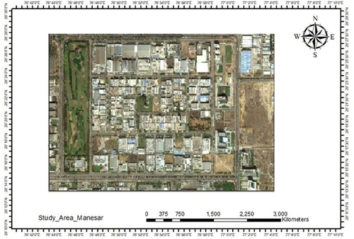
The study area lies at 28°22‘6.48“N, 76°55’35.47“E in the north Indian state of Haryana (Figure 1). The corridor is present in sector-5 of the Manesar Industrial area in the Gurugram district. The study area includes 4 km of road corridor which allows traffic in both directions. The area is well developed, and the roads are paved with no ongoing construction activities. The width of the road corridor is 40 ft and is found suitable for GNSS and photo data acquisition due to moderate traffic conditions. The road is having low vegetation cover and less count of high-rise buildings which helps us during GNSS data acquisition to avoid any signal multipath and visualization from satellite imagery.

Figure 1. Study area (mapping corridor) in Manesar Tehsil of Haryana, India.

3. Methodology

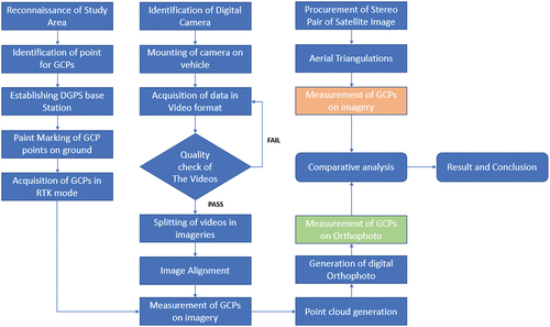
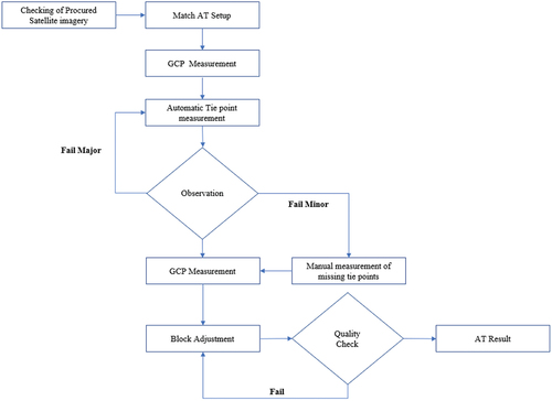
Based on the objective of the study, the method has been defined in four distinct parts (Figure 2). The first work part includes acquisition of GNSS and photo data of study area, and second part includes post-processing of acquired data and creation of digital orthophoto. The third part includes procurement and processing of stereo pair of satellite imagery, and the fourth part includes the comparative analysis of accuracy and cost of digital orthophoto and stereo satellite imagery.

Figure 2. Workflow of the adopted method.

3.1. Field investigation

The study area is a densely populated area with major factories and other production establishments. Industrial Model Township, Manesar Golf course lies next to sector-5. Roads are 40 ft wide for driving and navigating the car. The larger width of the road helps to better capture the dataset. Roads are paved with painted road markings. Before starting of differential global positioning system (DGPS) survey, reconnaissance of the area of interest was done in detail (Dashora et al. 2006). It is a surveying activity, where the area of interest is studied in detail with regard to the existing reference points, existing terrain and accessibility to know about the ground zero condition (Ferrer-González et al. 2020). It also includes testing of radio equipment and setting up the length up to which the base segment of radio can communicate with rover segments without interruption. The availability of satellite signals that may come up as a challenge due to signal multipath was assessed.

3.2. Establishing and acquiring ground control points (GCP)

GCPs are used for georeferencing of 3D point cloud in photogrammetric processes. It is also used in the comparison of accuracy of the final product such as Digital Terrain Model (DTM), DSM and orthophoto (John, 2012). GCPs can be either permanent ground features or reference targets scattered on the ground before the acquisition of the imagery (Ferrer-González et al. 2020).

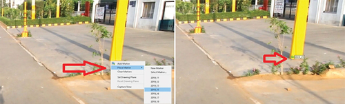
The GCPs (Mutluoğlu et al., 2015) were planned using Google Earth, where evenly distributed points were marked along the road corridor throughout the area of interest (Figure 3). Care was taken to plan the GCPs so that they fall at the road intersections and equal distance with clear visibility from one GCP to another to avoid satellite signal multipath. GCPs were captured at locations that can be easily recognized in the terrestrial and satellite images (Wang et al. 2012). Typically, square boxes were made for easy identification and measurement. Keeping this in mind, we set up most point locations at the edge or on the painted markings of the road. Pre-marking the locations was carried out by painting and writing the control point names for each location. Pre-marking helped in the identification of GCP points on captured imagery (DSLR) at a later stage of processing. The extent of accuracy requirements may vary from the project aim, but it was good enough to be within our scope of the study. Our aim of GCP data acquisition was to improve the accuracy of the orthophoto, aerial triangulation of satellite imagery and comparative assessment for the positional accuracies of the GCPs vs satellite imagery and produced orthophoto.

Figure 3. Distribution of GCPs on Google Earth and spider diagram from base location.

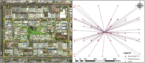
Control points were named at well-defined points such as edge of painted strips on the road with markings clearly painted. The control points were collected using a Trimble Spectra 80 DGPS instrument. The control points were measured as the real-time kinematics solution. The achieved accuracy of the GCPs was 1 cm, measured on ground. In challenging environments, GNSS signals using the SP80‘s Z-Blade GNSS-centric technology provide fast and reliable positioning. Among the available positioning modes are global positioning system (GPS) alone, GLONASS alone and BeiDou alone. The base station was stationed at the Survey of India tertiary point. A total of 59 GCPs were acquired on the ground. Forty-three GCPs were used for aerial triangulation of the mobile imagery, while seven GCPs were used as a checkpoint to evaluate the accuracy of the triangulated mobile imagery. For aerial triangulation of satellite imagery, six GCPs were used, while three GCPs were used as checkpoints to evaluate the accuracy.

3.3. Acquisition of digital photo

3.3.1. Choice of camera

The cameras used for our study are Canon electro optical system (EOS) 70D (Kissiyar et al., 2008) which is having 20.2 megapixels with advanced photosystem type-C (APS-C) CMOS-sensor and built in Wi-Fi and have digital imaging integrated circuit (DIGIC) 5+ image processor with ISO-range of 100–12800 (H: 25600) with electronic shutter. CMOS-sensor stands for complementary metal oxide semiconductor that converts the light into electrical signals. It allows shooting in a wide variety of lighting conditions. The touchscreen is 3-inches with 19-point cross type auto focus and 7.0 fps continuous burst shooting. Canon’s EOS 70D captures a massive 5472 × 3648-pixel resolution, which is good enough for even the largest enlargements and offers the best quality for significant cropping, while preserving the essence and detail of the scene. 14-bit signal processing ensures excellent tonal gradation and a wide (the International Organization for Standardization) range of 100–12800 (H: 25600) ensures excellent image capture even in dim lighting situations. Canon’s EOS 70D uses the DIGIC 5+ Image Processor to enhance the camera’s image sensor for faster data processing, improved noise reduction and even real-time compensation for chromatic aberration.

3.3.2. Mounting of camera for data acquisition

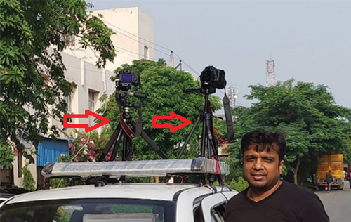
The initial tests from the fixed known positions on the ground with the camera axis horizontal or nearly horizontal did not bear any satisfactory results. It was due to the presence of open sky, which prohibited correlation. Thus, it was concluded to mount the cameras on the top of a vehicle and incline it at an angle of 25–30° (Figure 4). This enables to get oblique images focussing on the ground features without having sky in the picture. The next challenge was capturing of images at defined locations which was identified as time consuming. To mitigate this, it was decided to capture the data in video mode and later split the same into images. To capture the complete road corridor within the instantaneous field of view (as in aerial images), two cameras were mounted on the vehicle top facing opposite directions.

Figure 4. Camera mounting on vehicle.

3.3.3. Video capture and image conversion

Videos were captured with both cameras at the same time using a frame rate of 25 and a shutter speed of 50 with variable aperture. Both the cameras were not synchronized mechanically or electronically; however; their position was aligned to get the best possible overlapping images for tie point measurement during triangulation. The videos were quality controlled for any blurring or smearing effect. The vehicle speed was kept below 20 km/h throughout the data capture. The road corridor for the area of interest was subdivided into 11 segments, and video acquisition was done separately. The overlapping imagery found during video acquisition was marked for elimination at a later stage of processing. The two cameras were positioned at a set distance apart to create a stereo setup that can capture stereoscopic views with ≥60% lateral overlap and 80% of forwarding overlap along the vehicle track. Using a mobile mapping vehicle travelling at 20 km/h in an urban area, and the camera’s frame rate of 25, stereoscopic views at 5 m intervals can be acquired efficiently with this technology (Ferrer-González et al. 2020). Splitting of the images from videos are carried out using Blender Software. Blender is an open-source software primarily used for 3D computer graphics. It is used in 3D modelling, texturing, video editing and animation as well.

3.4. Post-processing of mobile imagery for production of orthophoto

The software used for generating the orthophotos is Agisoft Metashape which is a standalone software to perform processing of digital images and generating the 3D spatial data to be used in various applications of GIS. Selection of software was done considering its low price and accuracy in generation of point cloud (Singh, Jain, and Mandla 2014; Rahaman and Champion 2019).

Metashape does not load photos until they are needed for 3D reconstruction, so it is necessary to filter photos that will be used for 3D reconstruction. Alignment of photos was done using ‘high-accuracy’ parameters with the option of generic and reference preselection. The key point limit was kept at 40,000 and the tie point limit at 4000. During the process, ‘adaptive camera model fitting’ was not used. The alignment of photos requires computed camera positions that result in the generation of the sparse point cloud. Here, after inspecting alignment results, incorrectly positioned photos were realigned. Upon completing the alignment step, the point cloud and estimated camera positions were exported for further processing.

3.4.1. Tie point measurement

The tie point measurement is the process of measuring common points between two imageries (Tapas, 2011) for stitching with each other in space. We have done the measurement by finding well-defined common points between two imageries using Metashape Software. GCPs were imported as X, Y, Z coordinates in Metashape. The projection system of universe transverse macerator (UTM) Zone 43 was used. The control points were covered in the maximum number of photos for better triangulation. Once the GCPs were imported, they usually fall at the nearest location. The control points were then correctly placed using the markers. Guided marker placement was used since they speed up the measurement process significantly and reduces the chance of incorrect marker placement. The markers for each control point were placed at a minimum of five photos, while the maximum measurements were done for 10 photos. More tie points were measured by placing the markers at clearly visible locations to augment the triangulation (Figure 5). Labelling of each marker was assigned as default name given by the software.

Figure 5. Tie point measurement for aerial triangulation.

3.4.2. Aerial triangulation

Aerial triangulation is the method of georeferencing the images using GPS, IMU tie points and control points. As part of this process, it is necessary to find tie points and GCPs, to transfer these points between image segments, to measure their coordinates in the image and to convert them into ground coordinates. Bundle block adjustment performs transformation of image coordinates into ground coordinates (Ferrer-González et al. 2020). Hence, a visual reconstruction can be refined to produce the best 3D structure and viewing parameter, such as a camera position and/or calibration. According to this approach, a parameter estimate is calculated by minimizing a cost function based on the modelling error, and the solution is enhanced with respect to both structure and camera variations. As part of bundle adjustments, lenses distortions, refractions and earth curvatures are all corrected.

There are two sets of parameters in camera modelling. Position of the camera is described by extrinsic parameter which includes the six parameters of the exterior orientation, the three rotation angles around the three camera axes and the three coordinates of the projection centre. Using GPS and IMU, the parameters of the exterior orientation can be measured directly. However, they are also estimated during photogrammetric processes. It is necessary to model the geometry and physics of the camera using intrinsic parameters. The intrinsic parameters are used to decide the direction of the projection ray to an object point, given an image point and exterior orientation data.

The calibrated camera’s intrinsic parameters also decide the camera’s interior orientation. Based on 2D pixel coordinates (u, v), the following linear model illustrates a camera projective mapping of 3D real-world coordinates (×, y, z) into 3D object space:

$\left(u,v,1\right)=A\left[RT\right]\left(x,y,z,1\right)T,$

where homogeneous coordinate notation is used.

$A=\left(\begin{array}{ccc}{f}_x& s& u_o\\ 0& f_y& v_o\\ 0& 0& 1\end{array}\right)$

It is the intrinsic matrix having five intrinsic parameters:

• f_x, f_y – focal length in terms of pixels

• u₀, v₀ – principle point coordinates

• and s signifies skew coefficient along (×) and (y) axes.

Linear camera model can cover another intrinsic camera parameter such as lens distortion that is considered as important. R and T are rotation matrix and translation vector, respectively, and they are the extrinsic parameters. To denote camera orientation, two different sets of angles are used: omega, phi, kappa and yaw, pitch, roll triplets. The above sets of parameters define transformation between real-world and camera coordinates. The difference comes from how the georeferenced system is defined: if the reference system is UTM projection, then orientation parameters are omega, phi and kappa, while yaw, pitch and roll are parameters for tangent plane. The adjustment which is also known as ‘Optimise Camera Alignment’ was carried out to achieve higher accuracies in calculating the camera external and internal parameters and to correct the possible distortions in the camera.

3.4.3. Point cloud generation and filtering

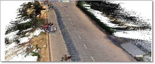
Point cloud generation was done using option ‘Build Dense Cloud’, in the Metashape package. The cloud density (Kraus and Pfeifer, 2001) is a function of maximum angle, maximum distance and cell size. The quality of the point cloud (Takai et al., 2013) can be defined as low, medium, and high. During generation, we considered the ‘high’ quality with advanced depth filtering (Snehmani et al., 2013) as ‘aggressive’ and colourized points for our study (Shan and Toth, 2008). The ‘high’ parameter ensures that maximum points are generated. Figure 6 represents the glance of point cloud generated during the study.

Figure 6. Point cloud generation output.

In addition to classification of dense point cloud (Gressin et al., 2012b), Metashape also allows generating and visualizing dense point cloud. It automatically divides all the points into two classes – ground points and the rest – and manual choice of a group of points to be placed in a certain class from the standard list known for LiDAR data (Hervieu and Soheilian, 2013b). Dense cloud point classification paves the way to customize Build Mesh step.

3.4.4. Automatic classification of ground points

Automatic classification was done using autodetection of ground points within the Metashape software. It consists of dividing dense point cloud (Wack and Wimmer, 2002) into cells of a certain size. First, approximation of DTM (Gianinetto, 2009) is done using the triangulation of the lowest point in each cell. Afterwards, new points are added to the ground class. The addition is done keeping in mind the two conditions; first, it should lie within a certain distance from the terrain model (Nelson et al., 2009) and second the angle between terrain models and the lines connecting this new point with a point from a ground class is less than a predefined angle. During our study, the maximum angle was 12°, a maximum distance of 0.5 m, and a cell size of 50 m was considered. The above iteration is carried out until all the points are checked. Now, base model is generated, and the dense point cloud is converted into a mesh.

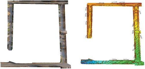
3.4.5. DEM and contour generation

A DEM is a surface model of height values at regular interval. Rasterization of DEM can be done from a dense point cloud, a sparse point cloud or a mesh. Heavy dense point cloud data gives the best result for rasterization. Distance, area, volume measurements and generating cross sections can be performed using the DEM-based points (Monnier et al., 2013) in Metashape. The DEM eases the generation of contours and can be depicted either over DEM or Orthomosaic within Metashape. DEM at 10 cm grid spacing (Crespi et al., 2006) is autogenerated using Metashape and manually edited to produce contours at 10 cm interval. Contours are validated and manually edited using Arc Info for crossings, finding isolated contours and any edge match errors.

3.4.6. Orthophoto generation

Orthomosaic export in Metashape software is typically used to create high-resolution imagery using the reconstructed surface model (Nurunnabi et al., 2013) and source photos. The most common application is aerial photographic survey data processing, but it is also used for UAV processing and any other terrestrial images. Metashape also allows to perform Orthomosaic (Zhao et al., 2020) seamline editing for better visual results. Orthorectification of images (Crespi et al., 2008) is the first step in generation of Orthomosaic. It removes the perspective distortions from the images using the DSM. The triangulated images are used to compute the 2.5D or 3D high-dense surface model. This method handles diverse types of terrain, as well as large volume of datasets. All the distances are preserved, and the Orthomosaic can be used for measurements (Ip, Mostafa, and El-Sheimy 2004; Lin et al. 2021; Vallet and Papelard 2015)

Orthomosaic involves adjusting the perspective of a camera and changing the scale according to distances between points on an object or the ground.

Generated DEM at 10 cm interval, as shown in Figures 7 and 8, and aerial triangulated imagery were processed for creation of digital orthophoto (DOP) at 2 cm GSD (Figures 7 and 8).

Figure 7. Generated orthophoto of road corridor at 2 cm GSD.

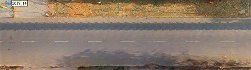
Figure 8. Digital orthophoto at 2 cm GSD and contour at 10 cm interval of road corridor.

Ortho errors not fixed by the DTM were resolved by manual editing. The final correction was done for image distortion and artefact removal on the road and its outside area.

There were various locations identified with non-coverage of DTM, which resulted in black pixels in the ortho, which was resolved by image editing.

4. Procurement and processing of satellite imagery

4.1. Procurement of stereo pair Cartosat imagery

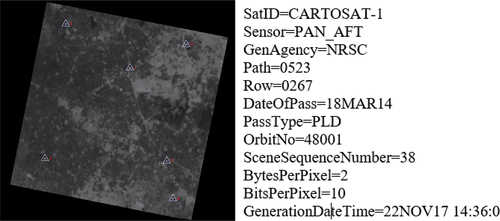
The first Indian Remote Sensing satellite, Cartosat-1, was launched on 5 May 2005 and is the 11th in the series (Singh et al., 2008). This Sun-synchronous satellite carries two panchromatic (fore/aft) cameras that capture along-track stereoscopic images over a 30 km swath at 2.5 m ground resolution with 10-bit radiometric resolution enabling the creation of correct 3D map. The satellite imagery of study area was obtained from the National Remote Sensing Centre with specifications as mentioned in Figure 9.

Figure 9. Cartosat-1 imagery specification.

4.2. Aerial triangulation of satellite imagery

The method adopted for this study is shown in Figure 10. GCP acquired using RTK mode was used for the aerial triangulation using Trimble INPHO, MATCH-AT software. A set of points (Toutin, 2004) were used as GCPs for satellite imagery triangulation, and another set was used as check points to confirm the AT result.

Figure 10. AT methodology.

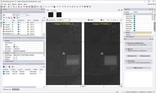
In MATCH-AT, project editor was used to import images, import GCPs and define scenes and projection system as shown in Figure 11. Image pyramid generation (Perez et al., 2003) was used for image overview. Six GCPs were used for AT block adjustment (Willneff et al., 2008) in one pair of Cartosat 2.5-m GSD imagery (Krishna et al., 2008).

Figure 11. MATCH -AT setup for aerial triangulation of Cartosat imagery.

The AT results after adjustment (Xiaobo et al., 1999) of the block were stored in *sattraing.log file. The log file shows all measurements of tie and GCP points and their residuals. During block adjustment, sigma value was 1.59807, and control point observation and residual obtained for all six GCPs are summarized in Table 1. The control points were acquired using Trimble Spectra GNSS receiver in RTK mode.

Table 1. Control point observation and residual.

Point ID	X	Y	Z	X-residual	Y-residual	Z-residual
1	683182.75	3142777.26	228.00	-0.42	0.32	-0.01
2	689207.37	3127488.01	255.00	-0.14	-0.39	0.13
3	692383.58	3146585.51	216.00	0.40	-1.38	0.54
4	672639.08	3149967.14	215.00	0.89	1.31	-0.41
5	669227.59	3127921.61	237.00	-0.31	0.64	-0.40
6	690228.08	3121323.19	264.00	-0.42	-0.50	0.15

5. Results and discussion

5.1. Accuracy assessment of the produced orthophoto

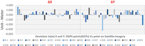
The accuracies of satellite imagery with respect to triangulated GCPs were measured (Muthry et.al 2008). Here, root mean square error (RMSE) was calculated based on deviation in XY coordinate between GCPs with the identified point on imagery (Table 2).

$RMSE=\sqrt{\frac{{\sum }_{i-1}^N{\left(Predicte{d}_i-Actua{l}_i\right)}^2}{N}}$

Table 2. RMSE value for DGPS observation and imagery.

S. no	Mean ΔX2	RMSE X	Max ΔX	Mean ΔY2	RMSE Y	Max ΔY
1	1.7748	1.3322	3.3688	3.9258	1.9814	2.9880

RMSE values for the DGPS observations and imagery are presented in Figure 12.

Figure 12. Deviation of XY between GCPs and aerial triangulated satellite imagery.

$\mathbf{R}\mathbf{M}\mathbf{S}\mathbf{E}={\left[{\mathbf{n}}^{-1}{\sum }_{\mathbf{i}=1}^{\mathbf{n}}{({\mathbf{Z}}_{\left(\mathbf{D}\mathbf{G}\mathbf{P}\mathbf{S}\right)}-{\mathbf{Z}}_{\left(\mathbf{I}\mathbf{m}\mathbf{a}\mathbf{g}\mathbf{e}\right)})}^2\right]}^{1/2}$

Afterwards, the accuracies of the produced orthophoto and the gCPs, measured by DGPS, were assessed. Here, RMSE was calculated based on deviation in XY coordinate between GCPs with the identified point on orthophoto (Table 3). A total of 59 GCPs were acquired on grounds; however, for the comparative analysis, 43 GCPs were used.

Table 3. RMSE value for DGPS observation and orthophoto.

S. no	Mean ΔX2	RMSE X	Max ΔX	Mean ΔY2	RMSE Y	Max ΔY
1	0.029	0.171	0.716	0.042	0.205	0.715

Similarly, the RMSE for the DGPS observations and orthophotos are presented in Figure 13.

Figure 13. Deviation of XY between GCPs and produced orthophoto.

$\mathbf{R}\mathbf{M}\mathbf{S}\mathbf{E}={\left[{\mathbf{n}}^{-1}{\sum }_{\mathbf{i}=1}^{\mathbf{n}}{({\mathbf{Z}}_{\left(\mathbf{D}\mathbf{G}\mathbf{P}\mathbf{S}\right)}-{\mathbf{Z}}_{\left(\mathbf{O}\mathbf{r}\mathbf{t}\mathbf{h}\mathbf{o}\right)})}^2\right]}^{1/2}$

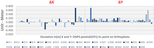
Our study brings the planimetric accuracy of the produced orthophoto at 2 cm pixel size using motion photogrammetry (mobile imagery) in terms of RMSE is 17 cm in X and 20 cm in Y. There are several studies available in the literature where high-resolution orthophoto (Grodecki and Dial, 2001) is produced using satellite imagery, aerial imagery and UAV for road corridor mapping. The accuracy of the data produced using the mobile mapping system is found 0.48 ± 0.23 m to 0.85 ± 0.52 m, which is very less compared with the accuracy achieved in our study. In a similar study (Toschi et al. 2015), the image acquisition phase was performed using a Nikon D3X digital camera where the system achieved a planimetric accuracy of 2.5 cm up to a range of 45 m. A comprehensive technique of usage of smartphones and CMOS cameras for the acquisition of imagery for building measurement was presented (Sadeq 2018). The study achieved an accuracy of orthophoto up to 7 cm. The study has the limitation of acquisition of photos in static mode and commercial implementation of the same in corridor mapping. However, our study does not have a dependency on data acquisition in static or mobile mode.

A comparison of the accuracy of orthophoto from mobile image and Cartosat -1 satellite image is presented in Figures 12 and 13. A study (Ashutosh et al. 2010) suggests that the accuracy of the Cartosat-1 imagery is decreasing with reducing the count of GCPs. Hence, for road corridor mapping, usage of satellite imagery for high-accuracy orthophoto brings the increased cost of GCPs. The method adopted in our study brings faster, low-cost and high-accuracy orthophoto.

5.2. Comparative assessment of cost for orthophoto production

Cartosat high-resolution satellite imageries have been obtained through National Remote Sensing Agency, India. The imageries are available in two components, one as fresh imageries of the latest date and another one as archived imagery. For our study, we procured archived stereo pair of satellite imagery.

Different pricing structures are offered for various products (Tables 4) and Table 5. To produce the orthophotos, one must have the mono/stereo imagery, DEM and GCPs. The total price for the latest imagery works out at USD122 per sqkm with a minimum of 100 sqm mandatory for procurement. This amounts to USD12200 as the bare smallest price for procurement without applicable taxes.

Table 4. Cost for fresh, archived Cartosat-1 imagery and orthophoto produced using developed method in our study.

Product/particulars	Cartosat-1 high-resolution satellite imageries-fresh in USD	Cartosat-1 high-resolution satellite imageries-archived (90 days) in USD	Terrestrial/mobile images from DSLR camera in USD
Mono, USD/100 sqkm	2750	1750	1250
Stereo, USD/100 sqkm	4000	2500
Image (stereo/ortho) processing, USD/100 sqkm	1389	1389	917
DEM 10X10m, USD/100km2	417	417	111
DSM, USD/100 sqkm	417	417	111
Orthophoto, USD/100 sqkm	5806	4306	222
GCP measurement, USD/100 sqkm	139	139	139
Min. price for procurement, USD/100 sqkm	12,167	9167	2750
Min. rate for procurement, USD/sqkm	122	92	28

Table 5. Comparative assessment of cost for imagery and mobile orthophoto.

Comparative assessment	Cartosat-1 high-resolution satellite imageries-fresh in USD	Cartosat-1 high-resolution satellite imageries-archived (90 days) in USD	Terrestrial/mobile images from DSLR camera in USD
% of price compared to fresh orthos	100	75	23
% of price compared to achieved orthos	133	100	30

The cost of orthophoto has been calculated for both field data acquisition and data processing done in-house. The first part of field data collection includes the acquisition of GCPs in RTK mode which takes less manual effort for the high-precision GCPs. The cost of the GCP acquisition was 13.9 USD per sqkm. The second part of data collection includes the acquisition of imagery using a locally hired DSLR camera and mobile vehicle. Including the capital expenditure and operational expenditure, the total cost of imagery acquisition was 12.50 USD per sqkm. This includes the cost of imagery data acquisition only and excludes the cost incurred during the testing phase of the study. The cost of data processing includes the cost of software licences for a year and is calculated based on the number of hours spent on each of the processes as summarized in Table 4. The unit price comes out to USD 28 per sqkm. To compare the cost with satellite imagery procurement, the price for orthophoto production was extrapolated to 100 sqkm. The cost comes at USD 2800 only.

The produced Orthomosaic at 2 cm GSD is cost effective (Table 5) in production as compared with fresh and archived satellite imagery.

6. Conclusions

In this article, we present a comprehensive overview of orthophoto production techniques, along with an overview of DEM, and orthophoto using DSLR cameras and GCPs. The accuracy of the obtained result has dependency on the accuracy of the GCPs and found within a tolerance of 20 cm in positional accuracy. This method is self-sustaining and ends the challenges of restrictions on data collection, for example, restrictions on flying photographic missions, continuous supply of data from earth observation satellites at an affordable price and responding to emergencies and other urgent needs to supply a quick turnaround of data. Our results and experience show that the technique is an inexpensive, effective and flexible approach to traditional photogrammetry. The method is having small cycle of data acquisition to processing and can be used by government department for utility-related work by getting data at periodic interval and analyse the development using change detection technique. Our study also infers that the cost of orthophoto production from mobile image is 77% cost-effective than the orthophoto cost from fresh/latest satellite imagery and 70% cost-effective than the orthophoto cost from archived imagery.

Acknowledgements

MD, SMV and MJ are grateful to Amity Institute of Geoinformatics and Remote Sensing (AIGIRS), Amity University, NOIDA, UP, India, for all the support. AK is thankful to the Department of Geology, BHU, for the assistance.

Disclosure statement

No potential conflict of interest was reported by the authors.

References

- Alan, W. L., M. Mostafa, and N. El-Sheimy. 2004. Fast Orthophoto Production Using the Digital Sensor System. doi:10.13140/2.1.1161.6967.
- Altmana, S., W. Xiaoa, and B. Graysona. 2017. “Evaluation of Low-Cost Terrestrial Photogrammetry for 3d Reconstruction of Complex Buildings’, Isprs Annals of the Photogrammetry, Remote Sensing and Spatial Information Sciences, Volume IV-2/W4.” ISPRS Geospatial Week 2017, Wuhan, China, 2017 September 18–22. pp.199–206
- Aparajithan, S., M. Donald, and J. Christophersona. 2012. ”Two Methods for Self-Calibration of Digitalt Camera“. International Archives of the Photogrammetry, Remote Sensing and Spatial Information Sciences. XXXIX (B1). Melbourne, Australia: ISPRS Archives. 25 August – 01 September 2012pp. 261–266
- Ashutosh, B., B. Enkhtur, S. Rahavendra, and S. Agrawal. 2010. ”Topographic Database Generation and 3D Feature Extraction Techniques Using Cartosat-1 Stereo Data“. Indian Cartographer, Journal of the Indian National Cartographic Association 30. Dehradun. November 10-12.
- Baiocchi, V., M. Crespi, L. De Vendictis, and A. Mazzoni. 2005. DSM Extraction from IKONOS and EROS a Stereo Imagery: Methodology, Accuracy and Problems. Proceedings of EARSeL Workshop 3D Remote Sensing, Porto, June 10-11.
- Birutė, R. 2005. “Performance Evaluation of Non-Metric Digitalt Camera for Photogrammetric Application.” Geodesy and Cartography 31 (1): 23–27.
- Bitenc, M., R. Lindenbergh, K. Khoshelham, and A. P. Van Waarden. 2011. “Evaluation of a LiDAR Land-Based Mobile Mapping System for Monitoring Sandy Coasts.” Remote Sensing 3 (7): 1472–1491. doi:10.3390/rs3071472.
- Christoph, S., J. Tian, R. Seitz, and P. Reinartz. 2013. ”Assessment of Cartosat-1 and WorldView-2 Stereo Imagery in Combination with a LiDar-DTM for Timber Volume Estimation in a Highly Structured Forest in Germany, Forestry.” An International Journal of Forest Research 86 (Issue 4): 463–473. October. doi:10.1093/forestry/cpt017.
- Crespi, M. G., F. Barbato, L. De Vendictis, F. Volpe, R. Onori, D. Poli, and X. Wang. 2008. “Orientation, Orthorectification, Terrain and City Modeling from Cartosat-1 Stereo Imagery: Preliminary Results in the First Phase of ISPRS-ISRO C-SAP.” Journal of Applied Remote Sensing 2: 023523.
- Crespi, M., L. De Vendictis, R. Onori, and F. Volpe. 2006. DSM Extraction from Quickbird Basic Stereo and Standard Orthoready Imagery: Quality Assessment and Comparison. Proceedings of 26th EARSeL Symposium New Developments and Challenges in Remote Sensing, Warsaw, 29 May- 2 June.
- Dashora, A., S. Bingi, B. Lohani, J. Malik, and A. A. Shah. 2006. “GCP Collection for CORONA Satellite Photographs: Issues and Methodology.” Journal of the Indian Society of Remote Sensing 34 (2): 2006. doi:10.1007/BF02991820.
- Dial, G. 2000. “IKONOS Satellite Mapping Accuracy.” ASPRS 2000 Proceedings, Washington DC, 2000 May 22-26.
- El-Halawany, S., A. Moussa, D. D. Lichti, and N. El-Sheimy. 2011. “Detection of Road Curb from Mobile Terrestrial Laser Scanner Point Cloud.” International Archives of Photogrammetry Remote Sensing and Spatial Information Sciences 2931: 29–31.
- Fanta-Jende, P., F. Nex, M. Gerke, and G. Vosselman. 2017. “Fully Automatic Feature-Based Registration of Mobile Mapping and Aerial Nadir Images for Enabling the Adjustment of Mobile Platform Locations in GNSS-Denied Urban Environments. ISPRS - International Archives of the Photogrammetry.” Remote Sensing and Spatial Information Sciences XLII-1/W1: 317–323. doi:10.5194/isprs-archives-XLII-1-W1-317-2017.
- Ferrer-González, E., F. Agüera-Vega, F. Carvajal-Ramírez, and P. Martínez-Carricondo. 2020. “UAV Photogrammetry Accuracy Assessment for Corridor Mapping Based on the Number and Distribution of Ground Control Points.” Remote Sensing 12 (15): 2447. doi:10.3390/rs12152447.
- Gianinetto, M. 2009. “Evaluation of Cartosat-1 Multi-Scale Digital Surface Modelling Over France.” Sensors (Basel, Switzerland) 9 (5): 3269–3288. doi:10.3390/s90503269.
- Gressin, A., C. Mallet, and N. David. 2012b. ”Improving 3D Lidar Point Cloud Registration Using Optimal Neighborhood Knowledge, ISPRS.” In ISPRS Annals of Photogrammetry, Remote Sensing and the Spatial Information Sciences. Vols 1-3, 111–116. Melbourne, Australia: ISPRS.
- Grodecki, J., and G. Dial. 2001. “IKONOS Geometric Accuracy.” Proceedings of Joint Workshop of ISPRS WorkingGroups I/2, I/5 and IV/7 on High Resolution Mapping from Space 2001, Hanover, Germany: University of Hanover, September 19-21.
- Hervieu, A., and B. Soheilian. 2013a. “Road Side Detection and Reconstruction Using Lidar Sensor.” In : IEEE Intelligent Vehicles Symposium (IV), Gold Coast, QLD, Australia, pp. 1247–1252.
- Hervieu, A., and B. Soheilian. 2013b. “Semi-Automatic Road/Pavement Modeling Using Mobile Laser Scanning.” ISPRS Annals of Photogrammetry, Remote Sensing and the Spatial Information Sciences II-3/W3: 31–36.
- Hervieu, A., B. Soheilian, and M. Bredif. 2015. “Road Marking´ Extraction Using a Model and Data-Driven RJ-MCMC.” ISPRS Annals of Photogrammetry, Remote Sensing and the Spatial Information Sciences II-3/W4: 47–54.
- Jauregui, L. M., and M. Jauregui. 2000. “Terrestrial Photogrammetry Applied to Architectural Restoration and Archaeological Surveys.” International Archives of Photogrammetry and Remote Sensing XXXIII (Part B5): 401–405.
- Joachim, H. 1996. ”Experiences with the Production of Digital Orthophotos.” Photogrammetric Engineering & Remote Sensing 62 (10) :1189–1194. October 1996.
- John, P. W. 2012. Digital Terrain Modeling. Geomorphology 137(Issue 1): 107–121. January 15.
- Khoshelham, K. 2005. ”Region Refinement and Parametric Reconstruction of Building Roofs by Integration of Image and Height Data , IAPRS.” In International Archives of Photogrammetry and Remote Sensing XXXVI (3-8). Vienna, Austria: IAPRS 6: XXXVI, part 3/W 24, 6.
- Kissiyar, O., T. Vanderstraete, R. Kroon, and B. Verbeke. 2008. ”Digital Cameras for a Photogrammetric Production Environment: A Test of the Geometric Stability and Accuracy.” The International Archives of the Photogrammetry, Remote Sensing and Spatial Information Sciences XXXVII (Part B1): 677–680. Beijing.
- Kraus, K., and N. Pfeifer. 2001. “Advanced DTM Generation from LiDAR Data.” International Archives of Photogrammetry Remote Sensing and Spatial Information Sciences 34 (3/W4): 23–30.
- Krishna Muthry, Y. V. N., S. Srinivasa Rao, D. S. Prakasa Rao, and V. Jayaraman. 2008. “Analysis of DEM Generated Using Cartosat-I Stereo Data Over Mausanne Les Alphilles – Cartosat Scientific Appraisal Programme (CSAP TS-5).” ISPRS 37: 1343–1348.
- Krishna, Y., S. Rao, D. Rao, and V. Jayaraman. 2008. “Analysis of DEM Generated Using Cartosat-1 Stereo Data Over Mausanne Les Alpiles – Cartosat Scientific Appraisal Programme (CSAP TS-5).” ISPRS Journal of Photogrammetry and Remote Sensing 37: 1343–1348.
- Kyriou, A., K. Nikolakopoulos, I. Koukouvelas, and P. Lampropoulou. 2021. “Repeated UAV Campaigns, GNSS Measurements, GIS, and Petrographic Analyses for Landslide Mapping and Monitoring.” Minerals 11 (3): 300. doi:10.3390/min11030300.
- Lin, Y. C., T. Zhou, T. Wang, M. Crawford, and H. Ayman. 2021. “New Orthophoto Generation Strategies from UAV-And Ground Remote Sensing Platforms for High-Throughput Phenotyping.” Remote Sensing 13 (5): 860. doi:10.3390/rs13050860.
- McElhinney, C., P. Kumar, C. Cahalane, and T. McCarthy. 2010. “Initial Results from European Road Safety Inspection (EURSI) Mobile Mapping Project.” International Archives of the Photogrammetry, Remote Sensing and Spatial Information Sciences 38 (Issue PART 5): 440–445.
- Monnier, F., B. Vallet, N. Paparoditis, J. P. Papelard, and N. David. 2013. “Registration of Terrestrial Mobile Laser Data on 2d and 3d Geographic Database by Use of a Non-Rigid ICP Approach.” ISPRS Annals of Photogrammetry, Remote Sensing and Spatial Information Sciences II-5/W2: 193–198.
- Mutluoğlu, Ö., M. Yakar, and H. Yilmaz. 2015. Investigation of Effect of the Number of Ground Control Points and Distribution on Adjustment at WorldView-2 Stereo Images. doi:10.13140/2.1.1158.2244.
- Nelson, A., H. I. Reuter, and P. Gessler. 2009. “DEM Production Methods and Sources.” In Geomorphometry: Concepts, Software, and Applications, edited by T. Hengl and H. I. Reuter, 65–85. Amsterdam: Elsevier.
- Nikolakopoulos, K., K. Soura, I. Koukouvelas, and N. Argyropoulos. 2016. “UAV Vs Classical Aerial Photogrammetry for Archaeological Studies.” Journal of Archaeological Science: Reports 14: 14. doi:10.1016/j.jasrep.2016.09.004.
- Nurunnabi, A., G. West, and D. Belton. 2013. “Robust Locally Weighted Regression for Ground Surface Extraction in Mobile Laser Scanning 3d Data.” ISPRS Annals of Photogrammetry, Remote Sensing and Spatial Information Sciences II-5/W2 (2): 217–222.
- Pech, K., N. Stelling, P. Karrasch, and H. G. Maas. 2013. “Generation of Multitemporal Thermal Orthophotos from UAV-Data.” ISPRS - International Archives of the Photogrammetry, Remote Sensing and Spatial Information Sciences XL-1/W2: 305–310. doi:10.5194/isprsarchives-XL-1-W2-305-2013.
- Perez, P., M. Gangnet, and A. Blake. 2003. ”Poisson Images Editing.” ACM Transactions on Graphics (TOG) 22 (number 3): 313–318. ACM.
- Peter, V. B. 1999. ”UAVs: An Overview Air & Space Europe Air & Space Europe ”. 1 (5–6): 43–47. september–December.
- Pu, S., M. Rutzinger, G. Vosselman, and S. O. Elberink. 2011. ”Recognizing Basic Structures from Mobile Laser Scanning Data for Road Inventory Studies.” ISPRS Journal of Photogrammetry and Remote Sensing 66 (6, Supplement): S28–39. Advances in LIDAR Data Processing and Applications.
- Qu, X., B. Soheilian, and N. Paparoditis. 2015. “Vehicle Localization Using Mono-Camera and Geo-Referenced Traffic Signs“. IEEE Intelligent Vehicles Symposium (IV) Seoul, South Korea, pp. 605–610.
- Rahaman, H., and E. Champion. 2019. “To 3D or Not 3D: Choosing a Photogrammetry Workflow for Cultural Heritage Groups.” Heritage 2 (3): 1835–1851. doi:10.3390/heritage2030112.
- Rottensteiner, F., and C. Briese. 2002. “A New Method for Building Extraction in Urban Areas from High-Resolution Lidar Data.” International Archives of Photogrammetry Remote Sensing and Spatial Information Sciences 34 (3/A): 295–301.
- Sadeq, H. 2018. Employing Smartphone and Compact Camera in Building Measurements. doi:10.23918/iec2018.11.
- Serna, A., and B. Marcotegui. 2013. “Urban Accessibility Diagnosis from Mobile Laser Scanning Data.” ISPRS Journal of Photogrammetry and Remote Sensing 84 (0): 23–32. doi:10.1016/j.isprsjprs.2013.07.001.
- Shan, J., and C. K. Toth. 2008. Topographic Laser Ranging and Scanning: Principles and Processing. Boca Raton, Florida: CRC Press.
- Singh, S. P., K. Jain, and V. R. Mandla. 2014. “Image Based 3D City Modeling: Comparative Study.” International Archives of the Photogrammetry, Remote Sensing and Spatial Information Sciences XL-5: 537.
- Singh, S. K., D. S. Naidu, T. P. Srinivasan, B. G. Krishna, and P. K. Srivastava. 2008. ”Rational Polynomial Modeling for Cartosat-1 Data.” The International Archives of the Photogrammetry, Remote Sensing and Spatial Information Sciences XXXVII (Part B1): 885–888.
- Snehmani, M.K. Singh, R.D. Gupta, A. Ganju. 2013. “Extraction of High-Resolution DEM from Cartosat-1 Stereo Imagery Using Rational Math Model and Its Accuracy Assessment for a Part of Snow-Covered NW-Himalaya.” Journal of Remote Sensing & GIS 4: 23–34.
- Tahar, K. N., and A. Ahmad. 2011. “Capability of Low Cost Digital Camera for Production of Orthophoto and Volume Determination.” Proceedings - 2011 IEEE 7th International Colloquium on Signal Processing and Its Applications, CSPA 2011. pp. 67–71. 10.1109/CSPA.2011.5759844.
- Takai, S., H. Date, S. Kanai, Y. Niina, K. Oda, and T. Ikeda. 2013. “Accurate Registration of Mms-Point Clouds of Urban Areas Using Trajectory.” ISPRS Annals of Photogrammetry, Remote Sensing and Spatial Information Sciences II-5/W2 (2): 277–282.
- Tapas, R. M. 2011. Detection of Landslides by Object-Oriented Image Analysis, ITC-Dissertation Number 189. Enschede, The Netherlands: University of Twente.
- Toschi, I., P. Rodríguez-Gonzálvez, F. Remondino, S. Minto, S. Orlandini, and A. Fuller. 2015. “Accuracy Evaluation of a Mobile Mapping System with Advanced Statistical Methods.” ISPRS - International Archives of the Photogrammetry, Remote Sensing and Spatial Information Sciences XL-5/W4. doi:10.5194/isprsarchives-XL-5-W4-245-2015.
- Toutin, T. 2004. ”Review Article: Geometric Processing of Remote Sensing Images: Models, Algorithms and Methods.” International Journal of Remote Sensing 25 (10) :1893–1924. 2004 May, 20.
- Vallet, B., and J. P. Papelard. 2015. “Road Orthophoto/Dtm Generation from Mobile Laser Scanning.” ISPRS Annals of Photogrammetry, Remote Sensing and Spatial Information Sciences II-3/W5: 377–384. doi:10.5194/isprsannals-II-3-W5-377-2015.
- Wack, R., and A. Wimmer. 2002. “Digital Terrain Models from Airborne Laserscanner Data-A Grid-Based Approach.” International Archives of Photogrammetry Remote Sensing and Spatial Information Sciences 34 (3/B): 293–296.
- Wang, J., Y. Ge, G. Heuvelink, C. Zhou, and D. Brus. 2012. “Effect of the Sampling Design of Ground Control Points on the Geometric Correction of Remotely Sensed Imagery.” International Journal of Applied Earth Observation and Geoinformation 18: 91–100. doi:10.1016/j.jag.2012.01.001.
- Willneff, J., T. Weser, F. Rottensteiner, and C. S. Fraser. 2008. ”Precise Georeferencing of Cartosat Imagery via Different Orientation Models.” The International Archives of the Photogrammetry, Remote Sensing and Spatial Information Sciences XXXVII (Part B1) 1287–1294. Beijing.
- Xiaobo, W., W. Shixing, and X. Chunsheng. 1999. A New Study of Delaunay Triangulation Creation [J]. Beijing: ACTA Geodaetica et Cartographic Sinica.
- Yu, L., Z. Xinqi, G. Ai, Z. Yi, and Y. Zuo. 2018. “Generating a High-Precision True Digital Orthophoto Map Based on UAV Images.” ISPRS International Journal of Geo-Information 2018 (9): 333. doi:10.3390/ijgi7090333.
- Zhao, Y., Y. Cheng, X. Zhang, S. Xu, S. Bu, H. Jiang, P. Han, K. Li, and G. Wan. 2020. “Real-Time Orthophoto Mosaicking on Mobile Devices for Sequential Aerial Images with Low Overlap.” Remote Sens 12: 3739. doi:10.3390/rs12223739.
- Zhao, G., and J. Yuan. 2012. “Curb Detection and Tracking Using 3d-Lidar Scanner.” In: Image Processing (ICIP), 2012 19th IEEE International Conference on, Seville, Spain (pp. 437–440). IEEE.