RS-DeepSuperLearner: fusion of CNN ensemble for remote sensing scene classification

ABSTRACT

Scene classification is an important problem in remote sensing (RS) and has attracted a lot of research in the past decade. Nowadays, most proposed methods are based on deep convolutional neural network (CNN) models, and many pretrained CNN models have been investigated. Ensemble techniques are well studied in the machine learning community; however, few works have used them in RS scene classification. In this work, we propose an ensemble approach, called RS-DeepSuperLearner, that fuses the outputs of five advanced CNN models, namely, VGG16, Inception-V3, DenseNet121, InceptionResNet-V2, and EfficientNet-B3. First, we improve the architecture of the five CNN models by attaching an auxiliary branch at specific layer locations. In other words, the models now have two output layers producing predictions each and the final prediction is the average of the two. The RS-DeepSuperLearner method starts by fine-tuning the five CNN models using the training data. Then, it employs a deep neural network (DNN) SuperLearner to learn the best way for fusing the outputs of the five CNN models by training it on the predicted probability outputs and the cross-validation accuracies (per class) of the individual models. The proposed methodology was assessed on six publicly available RS datasets: UC Merced, KSA, RSSCN7, Optimal31, AID, and NWPU-RSC45. The experimental results demonstrate its superior capabilities when compared to state-of-the-art methods in the literature.

KEYWORDS:

• Remote sensing
• scene classification
• deep learning
• ensemble fusion
• RS-DeepSuperLearner

1 Introduction

Classification of optical Very High Resolution (VHR) images is a crucial research problem in remote sensing (RS) (Cheng et al. 2020). Optical VHR images have many limitations. For example, they are affected by weather conditions, as they cannot be collected at night or under a cloud cover. Other challenges are related to geometric accuracy of the data and its positioning in a common reference system. In addition, because of the much higher resolution, it is no longer feasible or meaningful to analyse the image at the pixel level. Instead, classification is now focusing on a per-object or a scene approach.

Classification of RS scenes from urban areas is a fundamental step in many important applications, such as urban planning (Anees et al. 2020; Lynch, Blesius, and Hines 2020; Wu, Gui, and Yang 2020), natural hazards detection (Zhang, Song, and Yu 2011; Kerle and Bobrowsky 2013; Goldberg et al. 2020), environmental monitoring (Nyamugama and Qingyun 2005; Ambrosone et al. 2019; Li et al. 2020), mapping (Rogan and Chen 2004; Yang et al. 2017; Li, Wang, and Jiang 2020), and object detection (Bin and Li 2004; Ammour et al. 2017; Amini et al. 2018; Li et al. 2020). It is a challenging topic due to a wide variety of man-made objects and scene complexity (Cheng et al. 2020). Deep learning solutions, in particular convolutional neural networks (CNN), are now the state-of-the-art solutions for classifying RS scenes (Cheng et al. 2020; Song et al. 2019; Cheng, Han, and Lu 2017). However, despite the fact that a large number of deep learning models have been developed for this problem, having a single one that performs perfect classification in all situations encountered by an RS analysis system is likely unattainable. For that reason, decision fusion methods are proposed to produce correct decisions with a given amount of input information (Ludmila 2014). Decision fusion methods are tailored to generate a single decision from multiple sensor or classifier decisions. Moreover, fusion can compensate for the deficiencies of one classifier by using one or more additional classifiers.

In this article, a method for the scene classification in remote sensing based on ensemble learning is proposed, where the predictions of five different CNN models are fused including: VGG16 (Karen and Andrew 2014), Inception-V3 (Szegedy et al. 2016), InceptionResNet-V2 (Szegedy et al. 2016), DenseNet121 (Huang et al. 2017), and EfficientNet-B3 (Tan and Le 2019). Many works that use these CNN models for scene classification have been published (Xia et al. 2017; Alhichri et al. 2018, 2018; Ajjaji et al. 2019; Alhichri 2018; Lasloum et al. 2021; Li et al. 2021, 2021; Li, Zhang, and Zhu 2021). Cheng et al (Cheng et al. 2020). have presented a good review of the state-of-the-art of RS scene classification. However, it is impossible to comprehensively review all proposed methods in one article. Instead, the literature review included here highlights some recent examples of work from each research problem type and direction, with a special emphasis on ensemble methods in RS scene classification.

Most works have dealt with supervised classification, where RS scenes are classified into predefined categories of one dataset used during training and testing the model. However, more and more research is now focusing on reducing the labelling effort using techniques like domain adaptation and few-shot learning. Domain adaptation aims to transfer training knowledge from a labelled source dataset to a target dataset that has a few labelled samples (semi-supervised) or is completely unlabelled (unsupervised). For example, in recent work by Lasloum et al (Lasloum et al. 2021), a multisource semi-supervised domain adaptation (SSDAN) approach was presented. SDDAN uses a CNN model with a prototypical layer for classification and trains the model on the labelled source dataset, the few labelled target samples, and the remaining unlabelled target samples. The optimized loss function combines the standard cross-entropy loss and an entropy loss computed using the unlabelled data.

Furthermore, few-shot learning reduces the labelling effort because it only needs a few labelled samples per class. However, unlike domain adaptation, it also assumes that the target dataset contains new classes unseen during the model training. For example, Li et al (Li et al. 2021). have proposed a zero-shot RS scene classification (ZSRSSC) paradigm based on locality-preservation deep cross-modal embedding networks (LPDCMENs). Zero-shot means here that the target dataset has no labelled samples; instead, the method uses the semantic information about the classes and matches that with the semantic information from the labelled source dataset. In their proposed method, Li et al (Li et al. 2021). have addressed the problem of class structure inconsistency between the two hybrid spaces (i.e. the visual image space and the semantic space) by designing a set of explainable constraints to optimize LPDCMENs. In another zero-shot learning work, the authors of (Li et al. 2021) have proposed a new remote sensing knowledge graph (RSKG) from scratch to support the inference recognition of unseen RS image scenes. They have generated a semantic representation of scene categories by representation learning of RSKG (SR-RSKG). Then, they have designed a novel deep alignment network (DAN) with a series of well-designed optimization constraints to achieve robust cross-modal matching between visual features and semantic representations.

However, few works have investigated the ensemble fusion approach in RS scene classification. In (Li et al. 2017), Li et al. have proposed a novel two-stage neural network ensemble model to address the problem of low classification accuracies due to lack of labelled data. They have used a pretrained CNN for feature extraction and then fed the output features to a Restricted Boltzmann Machine (RBM) retrained network to get better feature representations. Finally, they have trained several copies of their deep model and then fused their outputs using an Ensemble Inference Network (EIN).

Moreover, Ye et al (Ye et al. 2019). have enhanced the performance of deep convolutional neural networks (D-CNN) by combining a Softmax loss function and a centre loss function and have built discriminative hybrid features using linear connections. Finally, they have adopted an ensemble extreme learning machine (EELM) classifier that classifies the hybrid features and fuses the classification results. Akodad et al (Akodad et al. 2019). have proposed a novel ensemble learning approach based on the concept of multilayer stacked covariance pooling (MSCP) of CNN features obtained from a pretrained model. Then, they have employed an ensemble learning approach among the stacked convolutional feature maps, which aggregates multiple learning algorithm decisions produced by different stacked subsets.

On the other hand, Alosaimi et al (Alosaimi and Alhichri 2020). built an ensemble of three state-of-the-art CNN classifiers: VGG-16, SqueezeNet, and DenseNet. They have fine-tuned the pretrained models then proposed a novel decision-level fusion approach that fuses the classification decisions using a combination of majority voting and breaking-ties confidence measure. The work by Tombe et al (Tombe, Viriri, and Dombeu 2020). presented a method using ensemble learning that fuses the outputs of CNN features using majority voting. First, they have fine-tuned a pretrained VGG-16 model for feature extraction. Then, they have used the multi-grain forest for feature learning and building an ensemble of classifiers. The final classification result is obtained by fusing the ensemble classifiers using majority voting. Another exciting work by Li et al (Li, Zhang, and Zhu 2021). has addressed the problem of wrong labels in an RS dataset. They have proposed a new remote sensing image scene classification error-tolerant deep learning (RSSC-ETDL) solution that adaptively combines an ensemble of CNN features to classify RS scenes and correct the labels of uncertain samples. To achieve these two goals simultaneously, they have alternatively performed the two tasks of training the multiple CNNs and correcting wrong labels iteratively.

Ensemble learning, which combines the results of a set of learning models rather than selecting a single classifier, is an old technique that has received a lot of attention in the machine learning literature (Dong et al. 2020). The types of ensemble learning approaches include bagging (Breiman 1996a; Bühlmann and Yu 2002), boosting (Schapire 1990; Freund and Schapire 1997), and stacking (Wolpert 1992; Breiman 1996b; Naimi and Balzer 2018). Bagging, the short form for bootstrap aggregating, is mainly applied in classification and regression. It increases the accuracy of models by using decision trees, which reduces variance to a large extent. The variance reduction improves accuracy and combats overfitting to the training data, which is a challenge for many predictive models (Garbin, Zhu, and Marques 2020). On the other hand, boosting is an ensemble technique that learns from previous predictor mistakes, resulting in better predictions in the future. It combines several weak base models to form one strong learning solution, thus significantly improving the predictability of models. Moreover, it works by arranging weak models in a sequence so that weak models can learn from the previous models in the sequence to create better predictive new models. Stacking, another ensemble method, is often referred to as stacked generalization. It allows a training algorithm to fuse several other similar learning algorithm predictions. Stacking has been successfully implemented and applied in regression, density estimations, distance learning, and classification. A basic common example of stacked generalization is averaging the outputs of several learning models. However, the averaging technique is not data-adaptive and is vulnerable to weak classifiers.

In the work by van der Laan et al (van der Laan, Polley, and Hubbard 2007; Polley and van der Laan 2010), stacked generalization with a cross-validation-based optimization framework was further extended. They have proposed SuperLearner, which uses cross-validation to examine different classifiers in the ensemble and, based on that evaluation, learns a better way to combine them. By minimizing the cross-validated risk, SuperLearner determines the optimal combination of a set of prediction algorithms or models. The individual models must provide different generalization patterns for ensemble fusion success; thus, diversity within the ensemble plays a crucial role in the training process. Otherwise, the ensemble would have the same predictions and provide as good accuracy as a single model. Van der Laan et al (Polley and van der Laan 2010; van der Laan and Dudoit 2003; van der Laan and Rubin 2006). have theoretically shown that the classifier with the best estimated cross-validated performance is asymptotically equivalent to the unknown best classifier in the ensemble if we assume independent and identically distributed data. Thus, cross-validation can be used as an objective measure to compare the performance of an set of classifiers.

This article proposes an ensemble fusion method to classify RS scenes, which we call RS-DeepSuperLearner. In particular, our approach fuses the predictions of five pretrained CNN models using another DNN, which is trained to perform the fusion. The inputs to the DNN are the predictions of the individual CNN models and their cross-validation accuracies. In this way, the RS-DeepSuperLearner has an objective approach of learning the fusion process, which should result in an increase in total classification accuracy following fusion. The main contributions of the article include the following:

• It proposes an effective ensemble learning method, called RS-DeepSuperLearner, to classify RS scenes that fuses the predictions of five pretrained CNN models: VGG16, Inception-V3, InceptionResNet-V2, DenseNet121, and EfficientNet-B3.

• It presents a novel way of modifying and fine-tuning the five pretrained CNN models by adding an auxiliary branch to the architecture which helps fight overfitting and increase diversity among models in the ensemble.

• It develops a novel DNN SuperLearner model that successfully fuses predictions of base models in the ensemble. Unlike previous work, the inputs to the proposed DNN SuperLearner are: 1) the class-predicted probabilities of each model, 2) the cross-validation accuracies for each class and for each base model, and 3) the overall accuracy of each base model.

The rest of the article is organized as follows. Section 2 describes the proposed RS-DeepSuperLearner method, presents the ensemble of CNN models and the architecture modifications, and describes the RS-DeepSuperLearner method in detail. Section 3 presents the experimental results. Finally, Section 4 shows the conclusions and future research.

2 Proposed approach

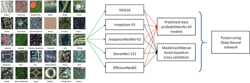
Figure 1 illustrates the main overview of the RS-DeepSuperLearner method. Five powerful CNN models are trained on the RS dataset. Then, a DNN is trained to fuse the predicted probabilities of all models into a final result. However, we will compare our method to basic stacked generalization algorithms, including naïve averaging and weighted averaging (Breiman 1996a, 1996b).

Figure 1. General overview of the RS-DeepSuperlearner method.

2.1 Description of the base CNN models

As previously stated, we constructed our classifier ensemble utilizing five alternative CNN models recently proposed in the literature. In our work, the selected base models are as follows: VGG16 (Karen and Andrew 2014), Inception-V3 (Szegedy et al. 2016), InceptionResNet-V2 (Szegedy et al. 2016), DenseNet-121 (Huang et al. 2017), and EffecientNet-B3 (Tan and Le 2019). These models have been used separately in many works for RS scene classification. However, to the best of our knowledge, no prior work has proposed fusing them. There are hundreds of CNN models proposed in the literature. Therefore, the number of possible ensemble combinations is very high and performing an exhaustive study will be impossible. What this study aims at is to create a deep SuperLearner network that outperforms other fusion methods and demonstrates that we can achieve high RS scene classification accuracy using the proposed ensemble method, which outperforms the state-of-the-art methods. Consequently, our choice for the CNN models is motivated by having as high diversity between the models as possible so that they will not make the same mistakes in their predictions.

First, we selected CNN models that belong to the following five main genres: networks with inception modules (Inception-V3), networks with residual connections (InceptionResNetV2), networks with dense connections (DenseNet121), networks with an optimized architecture (EfficientNet-B3), and a basic genre (VGG16). To increase diversity, the models we selected have different numbers of weights and layers and top-5 accuracy rates on the ImageNet dataset, as shown in Table 1. Moreover, Figure 2 presents a visual illustration of CNN models’s diversity. Each model is depicted as a pie chart with relative sizes of each property (normalized between zero and one). The pies on the figure look, and probably taste, different.

Figure 2. Diversity illustration of the CNN models used in the RS-DeepSuperlearner method.

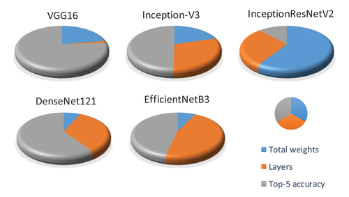
Table 1. Summary of base CNN models used in the RS-DeepSuperlearner ensemble method.

CNN model	Architecture	Total weights	Layers	Top-5 accuracy
VGG16	Basic CNN	14.7M	23	92.70%
Inception-V3	Inception block	22.7M	436	94.49%
InceptionResNetV2	Inception and residual connections	55.8M	393	87.10%
DenseNet121	Dense connections	7.7M	320	92.29%
EfficientNetB3	Inverted Residual and squeeze-excitation	11.7M	789	95.50%

Given this diversity, we expect a high probability that for each RS scene, at least one of these CNN models makes the correct class prediction. Additionally, the proposed RS-DeepSuperLearner has the role of intelligently exploiting this fact to produce improved class predictions.

All five CNN models used are pretrained on the ImageNet dataset (Deng et al.), the largest image classification dataset with over 14 million images divided into 1000 object classes. We always remove a few top layers for all of these pretrained models and replace them with our new layers to adapt the model to our classification problem which does not have 1000 classes as in ImageNet. The output layer is a fully connected layer with a Softmax activation function that produces the class probabilities. For some models we added another auxiliary branch with a separate output layer also having a Softmax activation function. Finally, we train the new model by fine-tuning all of its parameters, except the VGG16 model, where we fine-tune only the newly added layers following the suggestion of (Ammour et al. 2017; Alhichri et al. 2018), which incidentally increases the diversity among the ensemble CNN members.

The added new layers include a combination of fully connected layers, convolutional layers, average pooling layers, BatchNormalization (BN), and activation layers. In particular, we have found that the Global Average Pooling (GAP) layer is a much more effective pooling layer for use towards the end of CNN models. Therefore, we use the GAP layer in all five pretrained models. BN layer is an important addition that is quite effective in combatting the problem of overfitting, hence enhancing the performance of the CNN model. Moreover, we apply the ReLU action function and its advanced variant, the LeakyReLU function.

2.1.1 VGG16

VGG-Net is a family of CNN models developed by the Visual Geometry Group at Oxford University, hence the name VGG, in 2014 by Karen Simonyan and Andrew Zisserman (Karen and Andrew 2014). The VGG16 variant consists of 16 weight layers: 13 convolutional layers and 3 fully connected layers. The convolution operation is conducted using a kernel of a 3 × 3 dimension. Its uniform architecture makes it very appealing in the deep learning community because it is easy to understand.

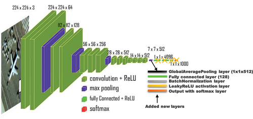
Figure 3 shows the modified VGG16 model. Here, we removed the top four layers from the pretrained VGG16 CNN model and then added our new layers. We started with the GAP layer. The GAP layer gets an input tensor of a size of $16\times 16\times 512$ and produces a tensor of a size of $1\times 1\times 512$. The next layer has 128 neurons that are FC to the GAP layer. The FC layer is followed by a BN layer and a LeakyReLU activation function with its alpha parameter set to 0.5.

Figure 3. Modified VGG16 architecture (14,783,573 total parameters and 2,428,437 trainable parameters).

2.1.2 Inception-V3 and InceptionResNet-V2

Inception networks are a family of CNN developed by Szegedy et al (Szegedy et al. 2015, 2016, 2016). The authors have engineered some tricks that set them apart from other conventional CNN architectures, such as AlexNet or VGG16. In 2014, the earliest version was introduced as GoogLeNet, also known as Inception-V1 (Szegedy et al. 2015). In 2015, Szegedy et al. improved their work by introducing a new BN layer in the second version, Inception-V2 (Szegedy et al. 2016), and the concept of factorizing convolutions in the third version, Inception-V3 (Szegedy et al. 2016). Finally, in another article, they have made further improvements in the Inception-V4 and the InceptionResNet versions (Szegedy et al. 2016). Inception-V4 contained several simplifications, which reduced the computational costs, whereas InceptionResNet-V2 included the concept of residual blocks inspired by the success of the ResNet architecture (He et al. 2016).

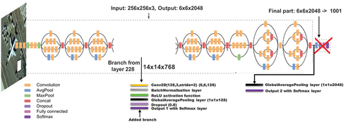
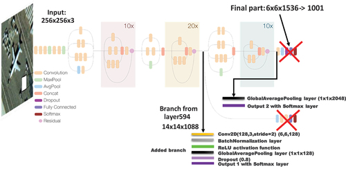
In this work, we selected the Inception-V3 and modified is as shown in Figure 4. We removed the top four layers. Then, we added a GAP layer, followed by the output FC layer with a Softmax activation function. Following the recommendation made by Bazi et al (Bazi et al. 2019), we also employed a second branch in the network connected to an intermediate layer of the CNN model, which has been quite effective in improving the performance of very deep models such as the one at hand. The second branch is connected to layer 228 of the original model and contains new layers, including convolutional, BN, ReLU activation, GAP, and Dropout layers, in addition to the final FC layer.

Figure 4. Modified Inception-V3 architecture (22,733,898 total params and 22,699,210 trainable).

As for InceptionResNet-V2 models, we modified as shown in Figure 5. The added layers are the same as in the Inception-V3 model, and the auxiliary branch is added starting from layer 594.

Figure 5. Modified InceptionResnet-V2 architecture (55,612,410 total params and 55,551,610 trainable).

2.1.3 DenseNet-121

DenseNet (Huang et al. 2017) is another family of CNN models that rely on the idea of dense connections, where each layer is connected to every other layer in a feedforward fashion. For each layer, the feature maps of all preceding layers are used as inputs, while its feature maps are used as inputs into all subsequent layers. In this work, we selected a version called DenseNet121, which provides a good compromise between accuracy and computational cost.

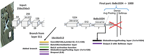
Figure 6 shows how we modified the DenseNet121 model. We removed the top three layers and added a GAP layer followed by the output FC layer with a Softmax activation function. As shown in Figure 6, we added a second branch similar to the Inception CNNs and connected it to layer 311.

Figure 6. Modified DenseNet121 architecture used (7,652,202 total params and 7,568,298 trainable).

2.1.4 EfficientNet-B3

EfficientNet is a new model scaling method recently developed by Tan et al (Tan and Le 2019). for scaling up CNNs. The model uses a simple greatly effective compound coefficient. Unlike traditional methods that scale dimensions of networks, such as width, depth, and resolution, EfficientNet scales each dimension with a fixed set of scaling coefficients uniformly. Practically, scaling individual dimensions improves model performance; however, balancing all network dimensions with respect to the available resources effectively improves the whole performance. The efficacy of model scaling depends strongly on the baseline network. To this end, a new baseline network is created using the automatic machine learning (AutoML) MNAS framework, which optimizes both precision and effectiveness (FLOPS) to perform a neural architecture search. Similar to MobileNetV2 (Sandler et al. 2018) and MnasNet (Tan et al. 2019), EfficientNet utilizes mobile inverted bottleneck convolution (MBConv) as the main building block. Furthermore, instead of the ReLU activation function, this network employs a new activation function known as Swish. The authors in (Tan and Le 2019) proposed eight versions, EfficientNet-B0 to EfficientNet-B7. In this work, we chose the EfficientNet-B3 version because it provides a good balance between performance and computational cost.

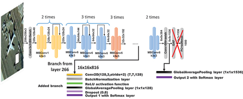
Figure 7 shows the modified EfficientNet-B3 model, where we removed the top two layers of the original model and then added the GAP and Softmax layers. The same second branch is also added as before and is connected to layer 266.

Figure 7. Modified EfficientNet-B3 architecture used (11,759,186 total params and 11,671,634 trainable).

2.2 Naïve unweighted averaging fusion

The simplest and most common way to combine the ensemble of classifiers is naïve unweighted averaging. Deep CNN classifiers are well known for having high variance and low bias in their results due to many randomization steps in the training data and the optimization algorithm. Naïve unweighted averaging is effective in reducing this variability.

In naïve unweighted averaging, we take the unweighted average of the output probability of the base classifiers. Equation 14(14) ${\vec{p}}_i\hspace{0.17em}=\hspace{0.17em}{F}_{\theta }\hspace{0.17em}\left(\hspace{0.17em}\overrightarrow{p_{i,1}}\hspace{0.17em},\overrightarrow{p_{i,2}}\hspace{0.17em},\dots \hspace{0.17em},\hspace{0.17em}\overrightarrow{p_{i,M}}\hspace{0.17em}\right),\hspace{0.17em}$(14) shows the predicted probability $p_{m,c}$ for the m^th classifier and class $c$ of a typical DNN based on the Softmax activation function:

(1) $p_{m,c}=softmax\left({\vec{a}}_m\right)\left[c\right]=\frac{{\vec{v}}_m\left[c\right]}{{\sum }_{\mathrm{c}=1}^{C}exp\left({\vec{v}}_m\left[c\right]\right)}$(1)

where $C$ is the number of classes and $\overrightarrow{v_m}$ = [$v_{m,1}$, $v_{m,2},\hspace{0.17em}$, $v_{m,C}$] is the output vector of the final layer before applying the Softmax activation function. Then, we computed the output probability of class $C$ using the naïve unweighted averaging as follows:

(2) $p_c=\frac{1}{M}\sum _{m=1}^M{p}_{m,c}$(2)

This can be rewritten in terms of $\overrightarrow{p_m}$ = [$p_{m,1}$, $p_{m,2}$, … , $p_{m,C}$] (i.e. all probabilities for the m^th classifier) as follows:

(3) $\vec{p}=\frac{1}{M}\sum _{m=1}^M\overrightarrow{p_m}$(3)

The deep learning literature has concluded that naïve unweighted averaging effectively reduces the variability of CNN models of similar architectures. However, it is not suitable for heterogeneous CNN models because it is vulnerable to weaker ensemble members (Zhao and Liu 2020). Some members in an ensemble of heterogeneous CNN models, may be weak in general, but they can outperform the others for certain classes or images. Thus, an intelligent combination approach should discover and capitalize on this observation.

2.3 Weighted-Averaging fusion

In this approach, the probabilities of $\mathrm{m}$ classifiers are fused using a weighted average, where the weights measure the confidence in the predictions of particular model (Breiman 1996b; Large, Lines, and Bagnall 2019). In other words, the contribution of each classifier to the final prediction is weighted by the classifier’s performance. In this technique, the new prediction probability is computed using a weighted average as follows:

(4) $p_c=\sum _{m=1}^M{w}_{m,c}{p}_{m,c}$(4)

where $w_{m,c}$ is the weight parameter for a particular classifier $\mathrm{m}$ and a particular class $\mathrm{c}$. To compute the weights, we use a cross-validation technique, where we divide the training set into $K$ folds and then hold one fold as a validation set while we use the rest of the folds for training (Large, Lines, and Bagnall 2019; Kohavi 1995; Benkeser et al. 2018). For a given fold k, we can compute the overall per-class accuracy $a_{\mathrm{k}}$ of the current classifier $m$ as follows:

(5) $\{a_{k,1}\hspace{0.17em}{a}_{k,2}\hspace{0.17em}{a}_{k,C}\},\hspace{0.17em}1\le \mathrm{k}\le \mathrm{K}$(5)

Thus, at the end of these $K$ experiments, we end up with many performance accuracies for each classifier, which can be averaged across $K$ validation sets to obtain the overall per-class accuracy of the m^th classifier:

(6) $A_m=\frac{1}{K}\sum _{k=1}^K{a}_{\mathrm{k}}$(6)

(7) $\hspace{0.17em}\{A_{m,1},A_{m,2},\hspace{0.17em}\dots \hspace{0.17em}{A}_{m,C}\}=\frac{1}{K}\sum _{k=1}^K\{a_{k,1},a_{k,2},\hspace{0.17em}\dots \hspace{0.17em}{a}_{k,C}\}$(7)

Finally, the weights per classifier $m$ and class $c$ are computed as follows:

(8) $w_{m,c}=\hspace{0.17em}\frac{A_{m,\mathrm{c}}}{{\sum }_{m=1}^M{A}_{m,\mathrm{c}}}$(8)

This ensures that the weights for a particular class $c$ sum to 1, i.e. ${\sum }_{m=1}^M{w}_{m,c}=1$.

2.4 Proposed RS-DeepSuperlearner method

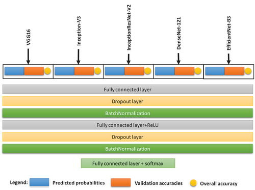
The SuperLearner is a type of stacking method, where the weights used to combine the different ensemble outputs are learned using another learning algorithm (van der Laan, Polley, and Hubbard 2007; Polley and van der Laan 2010). The SuperLearner uses cross-validation to make objective evaluation of the individual ensemble classifiers and based on that optimizes the fusion of the classifier ensemble. In this study, we propose to use DNN as a SuperLearner as shown in Figure 8, giving us the name RS-DeepSuperLearner. However, unlike previous work in (van der Laan, Polley, and Hubbard 2007; Polley and van der Laan 2010), the inputs to the proposed DNN SuperLearner are: 1) the class-predicted probabilities of each model, 2) the cross-validation accuracies for each class and for each base model, and 3) the overall accuracy of each base model. Below, we present the mathematical formulation of the proposed fusion algorithm using a DNN SuperLearner.

Figure 8. Architecture of the proposed DNN SuperLearner.

Recall that the training data are divided into K folds; then, the total cross-validated loss for a particular classifier m can be defined as follows:

(9) $L_{cv}^m=\sum _{d=1i}^K\sum _{\in val\left(d\right)}^{\hspace{0.17em}}loss\left(y_i,{\vec{p}}_{i,m}^{-d}\right)$(9)

where $val\left(d\right)$ is the samples in fold $d$ and ${\vec{p}}_{i,m}^{-d}$ is defined as the prediction vector of the $i^{th}\hspace{0.17em}$ sample by the $m^{th}\hspace{0.17em}$ base classifier, which is trained on all the training set except the $d^{th}\hspace{0.17em}$ fold. Thus, if we compute the final predicted probability for sample image $i$ using Equation 14(14) ${\vec{p}}_i\hspace{0.17em}=\hspace{0.17em}{F}_{\theta }\hspace{0.17em}\left(\hspace{0.17em}\overrightarrow{p_{i,1}}\hspace{0.17em},\overrightarrow{p_{i,2}}\hspace{0.17em},\dots \hspace{0.17em},\hspace{0.17em}\overrightarrow{p_{i,M}}\hspace{0.17em}\right),\hspace{0.17em}$(14) ,

(10) ${\vec{p}}_i^{-d}=\sum _{m=1}^M{\alpha }_m{\vec{p}}_{i,m}^{-d}$(10)

where $\vec{\alpha }\hspace{0.17em}=\left[\hspace{0.17em}{\alpha }_1\hspace{0.17em},{\alpha }_2\hspace{0.17em},\hspace{0.17em}\dots \hspace{0.17em},{\alpha }_M\hspace{0.17em}\right]$ are weights to be learned, then the total loss for the combined classifier can be expressed as follows:

(11) $L_{cv}^{\hspace{0.17em}}\left(\vec{\alpha }\right)=\sum _{d=1i}^K\sum _{\in val\left(d\right)}^{\hspace{0.17em}}loss\left({\vec{y}}_i,\sum _{m=1}^M{\alpha }_m{\vec{p}}_{i,m}^{-d}\right)$(11)

Then, the goal of the SuperLearner algorithm is to find the optimal weight vector that minimizes the above loss function; i.e.

(12) ${\vec{\alpha }}_{optimal}=\underset{\vec{\alpha }}{argmin}{L}_{cv}^{\hspace{0.17em}}\left(\vec{\alpha }\right)$(12)

This is a convex optimization problem that can be solved directly. In the above original formulation found in (van der Laan, Polley, and Hubbard 2007; Polley and van der Laan 2010), we have a total of M weights to optimize or one weight per classifier. However, varying the weights depending on each class $c$ and each sample image $i$ will be more effective. In this way, the weights will be more adaptive to each class and each image hopefully giving better results. Thus, in our proposed RS-DeepSuperLearner algorithm, we define the loss function as follows:

(13) $L_{cv}^{\hspace{0.17em}}\left(\hspace{0.17em}\vec{\alpha }\hspace{0.17em}\right)=\sum _{d=1i}^K\sum _{\hspace{0.17em}\in \hspace{0.17em}val\left(d\right)}^{\hspace{0.17em}}loss\left(\hspace{0.17em}{\vec{y}}_i,\hspace{0.17em}\sum _{m=1}^M{\vec{\alpha }}_{i,m}\odot \hspace{0.17em}\hspace{0.17em}{p}_{i,m}^{-d}\hspace{0.17em}\right)\hspace{0.17em},$(13)

where ${\vec{\alpha }}_{i,m}\hspace{0.17em}$ is the vector of $C$ (classes) weights for each sample image $i$ and classifier $m$ and ʘ means element-wise multiplication.

In our proposed RS-DeepSuperLearner, we use a deep neural network to solve this optimization problem. The DNN model learns the nonlinear mapping between the prediction probabilities of the base classifiers and the final combined prediction probabilities, such that

(14) ${\vec{p}}_i\hspace{0.17em}=\hspace{0.17em}{F}_{\theta }\hspace{0.17em}\left(\hspace{0.17em}\overrightarrow{p_{i,1}}\hspace{0.17em},\overrightarrow{p_{i,2}}\hspace{0.17em},\dots \hspace{0.17em},\hspace{0.17em}\overrightarrow{p_{i,M}}\hspace{0.17em}\right),\hspace{0.17em}$(14)

where $\theta$ represents the set of parameters of the DNN model. The set $\theta$ can have thousands of parameters, much more than M weights in the weighted-averaging approach in Section 2.3. This makes it more adaptive to each class and each image, and hopefully, it will find a more optimal combination of the classifier ensemble.

Another contribution of this article is adding the validation accuracies for all base classifiers ${\vec{A}}_m\hspace{0.17em}=\left[\hspace{0.17em}{A}_m\hspace{0.17em},\hspace{0.17em}{A}_{m,1}\hspace{0.17em},\hspace{0.17em}{A}_{m,2}\hspace{0.17em},\dots \hspace{0.17em},\hspace{0.17em}{A}_{m,C}\hspace{0.17em}\right]$ as an input to the DNN to provide it with more information to learn from. Thus, in summary, the proposed RS-DeepSuperLearner method uses a DNN model $F_{\theta }$ that learns the following mapping:

(15) ${\vec{P}}_i\hspace{0.17em}=\hspace{0.17em}{F}_{\theta }\hspace{0.17em}\left(\hspace{0.17em}\overrightarrow{p_{i,1}}\hspace{0.17em},\overrightarrow{p_{i,2}}\hspace{0.17em},\dots \hspace{0.17em},\hspace{0.17em}\overrightarrow{p_{i,M}}\hspace{0.17em},\hspace{0.17em}{A}_m\hspace{0.17em},\hspace{0.17em}{A}_{m,1}\hspace{0.17em},\hspace{0.17em}{A}_{m,2}\hspace{0.17em},\dots \hspace{0.17em},\hspace{0.17em}{A}_{m,C}\hspace{0.17em}\right),\hspace{0.17em}$(15)

where ${\vec{P}}_i\hspace{0.17em}$ is the final fused predicted class probabilities for sample image $i$. The DNN SuperLearner is illustrated in Figure 8, which shows that it is composed of two hidden fully connected layers. Each layer is followed by a BatchNomalization layer and a ReLU activation faction. Moreover, we have experimented with an additional Dropout layer after the first hidden layer. Both BatchNomalization and Dropout effectively fight overfitting in DNN models (Garbin, Zhu, and Marques 2020). We conducted experiments to investigate their effectiveness in our case.

3 Experimental results

This section presents an extensive experimental analysis to show the capabilities of the proposed solution.

3.1 Dataset description

In total, seven datasets were used to test our method: the University of California Merced (UCMerced) dataset (Yang and Newsam 2010), the Kingdom of Saud Arabia (KSA) dataset (Othman et al. 2017; Alhichri 2020a), the RSSCN7 dataset (Zou et al. 2015a), the Optimal-31 dataset (Wang et al. 2019), the Aerial Image Datasets (AID) dataset (Xia et al. 2017), and the NWPU-RESISC45 dataset (Cheng, Han, and Lu 2017). We present detailed information of each dataset: moreover, Table 2 summarizes their properties.

Table 2. Summary of RS datasets.

Dataset	No. of images	No. of classes	Images/class	Image size	Resolution	Data source	Year
UC Merced	2,100	21	100	256 × 256	0.3 m/pixel	Aerial orthoimagery	2010
KSA	3,250	13	250	256 × 256	Variable	Multisensor	2012
RSSCN7	2,800	7	400	400 × 400	N/A	Google Earth	2015
AID	10,000	30	220–420	600 × 600	0.5–8 m/pixel	Google Earth	2017
NWPU-RESISC45	30,000	45	700	256 × 256	0.2–30 m/pixel	Google Earth	2017
Optimal-31	1,860	31	60	256 × 256	0.5 m/pixel	Google Earth	2018

UC merced dataset

The UC Merced land-use dataset comprises 2,100 overhead scene images divided into 21 land-use scene classes. Each class consists of 100 aerial images measuring 256 × 256 pixels, with a spatial resolution of 0.3 m per pixel in the red-green-blue (RGB) colour space. This dataset was extracted from aerial orthoimagery downloaded from the United States Geological Survey (USGS) National Map.

KSA dataset

This multisensor dataset (Li et al. 2020) was acquired over different cities of KSA (i.e. Riyadh, Al-Qassim, Al-Rajhi farms, Al-Hufuf, and Jeddah) by three different VHR sensors, IKONOS-2, GeoEye-1, and WorldView-2, with spatial resolutions of 1 m, 0.5 m, and 0.5 m, respectively. This dataset consists of 3250 RGB images of a size of 256 × 256 pixels categorized into 13 classes (250 images per class). The class labels are as follows: agriculture, beach, cargo, chaparral, dense residential, dense trees, desert, freeway, medium-density residential, parking lot, sparse residential, storage tanks, and water. This dataset can be downloaded from here

RSSCN7

This dataset (Zou et al. 2015b) contains 2800 remote sensing images collected from Google Earth and is divided into seven scene categories: grassland, forest, farmland, parking lot, residential region, industrial region, and river and lake. Each category consists of 400 images with a size of 400 × 400 pixels.

Optimal-31

This new dataset contains images from Google Earth imagery. The images have a size of 256 × 256 pixels and their resolution is 0.5 metres. Optimal-31 categorizes 1860 images within 31 classes, each class containing 60 images (Li, Wang, and Jiang 2020).

Aerial image datasets (AID)

This dataset (Ambrosone et al. 2019) is a collection of 10,000 annotated aerial images distributed in 30 land-use scene classes and can be used for image classification purposes. Compared with the UC Merced dataset, AID contains more images and covers a wider range of scene categories, thus being in line with the data requirements of modern deep learning.

NWPU-RESISC45

NWPU-RESISC45 is acquired from Google Earth imagery, created by Northwestern Polytechnical University (NWPU) (Wu, Gui, and Yang 2020). It consists of 31,500 remote sensing images, divided into 45 classes. Each class has 700 images with a cropped size of 256 × 256 pixels. Most of the classes with spatial resolutions vary from around 30 metres to 0.2 metres, except for those having lower spatial resolutions: island, lake, mountain, and snowberg.

3.2 Experimental setup

We implement all our models in the Google Colab environment using the Tensorflow machine learning library. Tensorflow is a neural network application programming interface written in Python. First, we have resized all datasets to a standard size of 256 × 256 pixels. The newly resized datasets can be downloaded from this web location (Alhichri 2020b). For performance evaluation, we present the results using the overall accuracy (OA), that is the ratio of the number of correctly classified samples to the total number of the tested samples. OA, is the metric used by almost all works on RS scene classification methods in the literature due to the fact that the classes in RS datasets are balanced. It is generally known in the machine learning literature that precision, recall, and F1 score are instrumental when we have unbalanced datasets, such as medical classification problems where the samples classified as a disease are scarce compared to the normal and other samples.

We split each dataset of images into training and testing sets for training the networks. The train/test splits used in the experiments 20%-80%, 50%-50%, and 80%-20%. However, we cannot test with large training sets due to limitations on computational resources for large datasets, such as the AID and NWPU-RESISC45 (see Table 2 for dataset sizes). For these datasets, we follow the footsteps of previous researchers by applying the method on 10%-90% and 20%-80% splits only. Moreover, we consider the 50%-50% split for the AID dataset

For the training parameters, we set the batch size to 32 images and train for 60 epochs. However, we divide the training epochs into three stages of 20 epochs each. Then, we employ a decaying learning rate strategy, such that the learning rate starts as 0.001 in the first stage and is reduced to 0.0001 and 0.00001 in stages two and three, respectively. This reduction is important to enhance the convergence of the model. Basically, because of the initial high learning rate, the model searches in a larger area of the search space. Then, when the best minimum of the loss function is found, we continue searching with a lower learning rate to more precisely locate the minimum value, which in turn fine-tunes the training of the model. Furthermore, we employ the ‘early-stopping’ technique in stage three (the last 20 epochs with learning rate 0.00001), which stops the training of the model if the loss value does not change for a given number of consecutive epochs (five epochs in our case).

3.3 Optimizing the DNN metalearning model

In this subsection, we conduct experiments to study the DNN SuperLearner model, where we focused on one dataset, namely, the NWPU-RESISC45 dataset, with a train-test split of 10%-90%, since it is a challenging dataset with the largest size.

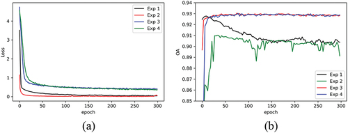
In the first set of experiments we train the DNN for 300 epochs with a batch size of 256 and the learning rate parameter for the Adam optimizer set to 0.001. We perform a total of 4 experiments in this set. In experiment 1, we only use two hidden FC layers with ReLU activation functions. Then, in experiment 2, we add BN layers after each FC layer. In experiment 3, we remove the BN layers and replace them with Dropout layers with a probability of 0.8. Finally, in experiment 4, we add both BN and Dropout layers to the model. Figure 9 plots the loss curve and the OA on the test data for the 300 epochs. We note that the experiments were conducted 30 times to produce these curves and the average loss and OA curves were computed. These results clarify that the BN and Dropout layers are effective in combatting overfitting as the OA on the test data is much better in experiments 3 and 4. Furthermore, we can conclude that Dropout is more important than BN layers because when we used BN layers only in experiment 2, the OA was worse.

Figure 9. Training DNN metalearning model: (a) loss curve for training data; (b) OA accuracy on the test data.

We recompile the model with a lower learning rate for the Adam optimizer equal to 0.0001 and then continue training the model for another 20 epochs to further enhance the OA accuracy. Finally, we execute this training for 30 times and fuse the predicted class probabilities using naïve averaging to reduce variability in the final results and also introduce further improvements.

3.4 Single-model results

First, Table 3 shows the results in terms of OA for each CNN model, our modified version trained separately, and all datasets. We also included the highest possible OA that can be achieved for each dataset. This is computed by considering the classification to be correct if at least one of the classifiers in the ensemble is correct. In other words, we are assuming that we have an oracle SuperLearner that can help us select the correct classifier all the time. Effectively, this represents an upper bound OA that can be obtained by fusing the given ensemble of models.

Table 3. Single-model OA for datasets and the upper bound OA when the correct model is always selected.

Dataset	Train ratio	VGG16 [ours]	Inception-V3 [ours]	InceptionResNet-V2 [ours]	DenseNet-121 [ours]	EfficientNet-B3[ours]	Upper bound OA
UC Merced	20%	91.85	90.42	93.45	92.86	94.64	98.75
	50%	95.24	96.48	97.62	98.00	98.29	99.71
	80%	96.90	97.38	98.57	99.29	99.76	100.00
KSA	20%	94.12	92.96	95.54	95.04	96.23	99.08
	50%	96.86	95.94	97.11	97.54	97.97	99.32
	80%	97.54	97.85	97.85	98.31	99.08	99.85
RSSCN7	20%	87.81	90.80	93.08	92.01	92.99	98.04
	50%	91.50	93.93	94.86	96.00	96.36	99.43
	80%	90.89	94.64	95.54	95.71	96.43	98.57
Optimal-31	20%	80.44	79.44	84.81	83.00	81.59	95.30
	50%	86.34	89.25	89.46	90.00	92.69	97.42
	80%	91.67	94.09	93.55	93.82	94.89	98.12
AID	10%	85.54	87.16	88.52	89.83	91.54	97.40
	20%	89.95	91.47	92.61	93.56	95.08	98.21
	50%	93.03	93.98	94.84	93.03	96.59	98.94
NWPU-RESISC45	10%	85.44	86.60	88.67	90.49	91.40	97.11
	20%	89.02	89.70	91.37	92.64	93.77	98.00

The upper bound OA is significantly higher than the OA by individual models (especially for the 20%-80% splits) and even reaches 100% in some cases. The impressive upper bound OA confirms the diversity of the selected CNN models because when they start to have wrong predictions, they are not all wrong for the same scenes; instead, in a significant portion of cases, at least one of the models is correct.

3.5 Comparison of our results with the state-of-the-art methods

In this section, we compare our results to those of other state-of-the-art methods published in the literature. Our proposed method has performed better than previous methods for all datasets except for UC Merced and AID datasets. The UC Merced dataset was compared with a large number of previous methods from the literature in Table 4. Our proposed method has outperformed all of them except for the BiMobileNet (MobileNetv2) (Yu et al. 2020) and HABNet methods (Yu et al. 2020), which have outperformed our method in the 20%-80% split. However, we have outperformed them for the other two splits because when we have a low number of images, the validation accuracies do not measure the performance of the models in the different classes well. Consequently, the RS-DeepSuperLearner’s ability to learn the best way to fuse the ensemble of CNN models is reduced.

Table 4. Comparison results for UC Merced RS dataset.

		Training ratio
Method	Year	20%	50%	80%
GoogLeNet+SVM (Xia et al. 2017)	2017		92.70±0.60	94.31±0.89
AlexNet (Liang, Monteiro, and Saber 2016)	2017			95.00±1.74
VGG-16+EMR (Wang et al. 2017)	2017			98.14
Fusion by Addition (Chaib et al. 2017)	2017			97.42±1.79
ResNet (Liang, Monteiro, and Saber 2016)	2017			97.19±0.57
SAL-TS-Net (GoogleNet) (Yu and Liu 2018b)	2018		97.79 ± 0.56	98.90 ± 0.95
D-DSML-CaffeNet (Gong et al. 2018)	2018			95.76±1.70
SPP-net+MKL (Liu et al. 2018)	2018			96.38
MCNN (Liu, Zhong, and Qin 2018)	2018			96.66±0.90
Triplet networks (Liu and Huang 2018)	2018			97.99±0.53
VGG-16 + IFK (Yu and Liu 2018a)	2018			98.57±0.34
OverfeatL + IFK (Yang, Mu, and Zhao 2018)	2018			98.91
VGG-16+MSCP (He et al. 2018)	2018			98.36±0.58
CAE ELM+CNN (Wang et al. 2019)	2019	90.18
Fine-tuned ResNet50 (Liu et al. 2019)	2019	74.11	89.43	91.90
Siamese ResNet50+RD (Zhou et al. 2019)	2019		91.71	94.50
WSPM-CRC (ResNet152) (Liu et al. 2019)	2019			97.95
CTFCNN (Huang and Xu 2019)	2019			98.44±0.58
ARCNet-VGG16 (Wang et al. 2019)	2019		96.81±0.14	99.12±0.40
CapsNet (Inception-v3) (Zhang, Tang, and Zhao 2019)	2019		97.59±0.16	99.05±0.24
DDRL-AM (ResNet18) (Li et al. 2020)	2019			99.05±0.08
Fine-tuning VGG16 (Sun et al. 2020)	2020		96.57±0.38	97.14±0.48
GBNet + global feature (Sun et al. 2020)	2020		97.05±0.19	98.57±0.48
FACNN (Lu, Sun, and Zheng 2019)	2019			98.81±0.24
BiMobileNet (MobileNetv2) (Yu et al. 2020)	2020	96.41±0.57	98.45±0.27	99.03±0.28
CAD+DenseNet (Tong et al. 2020)	2020		98.57±0.33	99.16±0.27
HABNet (Yu et al. 2020)	2020	96.95±0.59	98.47±0.47	99.29±0.35
Ensemble methods:
Two-stage NN ensemble (Li et al. 2017)	2017			95.11
HDF-EELM (Ye et al. 2019)	2019		98.14 ± 0.31	99.41 ± 0.36
Ensemble CLP (Akodad et al. 2019)	2019		97.4 ± 0.3%
Multigrained Forest ensemble (Tombe, Viriri, and Dombeu 2020)	2020			96.85
CNN ensemble MV+Breaking Ties (Alosaimi and Alhichri 2020)	2020	93.93%
Fine-tuning VGG16 [ours]		91.85	95.24	96.90
Fine-tuning Inception-V3 [ours]		90.42	96.48	97.38
Fine-tuning InceptionResNet-V2 [ours]		93.45	97.62	98.57
Fine-tuning DenseNet-121 [ours]		92.86	98.00	99.29
Fine-tuning EfficientNetB3 [ours]		94.64	98.29	99.76
Fusion naïve-averaging [ours]		95.71	98.38	99.29
Fusion weighted-averaging [ours]		95.71	98.38	99.29
Fusion majority voting [ours]		95.42	98.38	99.05
RS-DeepSuperLearner [ours]		95.95	98.57	99.52

The KSA, RSSCN7, Optimal-31, and NWPU-RESISC45 datasets are also compared as shown in Tables 5, 6, 7, and 8, respectively. Our method has outperformed listed methods from the literature for all these datasets.

Table 5. Comparison results for KSA RS dataset.

		Training ratio
Method	Year	20%	50%	80%
CS Multifeature Fusion (Zhao, Tang, and Huo 2014)	2014		91.69	90.77
Pretrained CNN+SAE (Othman et al. 2016)	2016		94.77	94.92
DAN with adaptation (Othman et al. 2017)	2017		94.36+0.41	95.33+0.79
Pretrained CNN+SVM (Othman et al. 2017)	2017		94.52	94.46
Multiinput SqueezeNet-Attn (Ajjaji et al. 2019)	2019	92.15	93.48
SqueezeNet-Attn (Alswayed, Alhichri, and Bazi 2020)	2020	94.25	96.62	96.77
Ensemble methods:
CNN ensemble MV+Breaking Ties (Alosaimi and Alhichri 2020)	2020	94.58%
Fine-tuning VGG16 [ours]		94.12	96.86	97.54
Fine-tuning Inception-V3 [ours]		92.96	95.94	97.85
Fine-tuning InceptionResNet-V2 [ours]		95.54	97.11	97.85
Fine-tuning DenseNet-121 [ours]		95.04	97.54	98.31
Fine-tuning EfficientNetB3 [ours]		96.23	97.97	99.08
Fusion naïve-averaging [ours]		96.81	98.15	98.77
Fusion weighted-averaging [ours]		96.77	98.09	98.77
Fusion majority voting [ours]		96.19	96.25	98.77
RS-DeepSuperLearner [ours]		96.62	98.15	99.38

Table 6. Comparison results for RSSCN7 RS dataset.

		Training ratio
Method	Year	20%	50%	80%
GoogLeNet (Xia et al. 2017)	2017	82.55±1.11	85.84±0.92
VGG-VD-16 (Xia et al. 2017)	2017	83.98±0.87	87.18±0.94
CaffeNet (Xia et al. 2017)	2017	85.57±0.95	88.25±0.62
Resnet + Hybrid-KCRC (Liu et al. 2018)	2018		98.37
TEX-Net-LF (Anwer et al. 2018)	2018	92.45±0:45	94.0±0.57
Fine-tune MobileNet V2 (Zhang, Zhang, and Wang 2019)	2019	89.04±0.17	92.46±0.66
WSPM-CRC (ResNet152) (Liu et al. 2019)	2019		93.90
SE-MDPMNet (Zhang, Zhang, and Wang 2019)	2019	92.65±0.13	94.71±0.15
Contourlet CNN (Liu et al. 2020)	2020		95.54±0.71
Dual Attention-Aware Net (Gao et al. 2020)	2020	91.07±0.65	93.25±0.28
Fine-tuning VGG16 [ours]		87.81	91.50	90.89
Fine-tuning Inception-V3 [ours]		90.80	93.93	94.64
Fine-tuning InceptionResNet-V2 [ours]		93.08	94.86	95.54
Fine-tuning DenseNet-121 [ours]		92.01	96.00	95.71
Fine-tuning EfficientNetB3 [ours]		92.99	96.36	96.43
Fusion naïve-averaging [ours]		94.06	96.79	96.25
Fusion weighted-averaging [ours]		94.15	96.79	96.25
Fusion majority voting [ours]		93.84	97.00	96.43
RS-DeepSuperLearner [ours]		94.33	96.93	96.61

Table 7. Comparison results for Optimal31 RS dataset.

Method	Year	Training ratio
		20%	50%	80%
VGG16 (Xia et al. 2017)	2017			89.12±0.35
Fine-tuning AlexNet (Wang et al. 2019)	2019			81.22±0.19
Fine-tuning GoogLeNet (Wang et al. 2019)	2019			82.57±0.12
ARCNet- AlexNet (Wang et al. 2019)	2019			85.75+0.35
Fine-tuning VGG16 (Wang et al. 2019)	2019			87.45±0.45
ARCNet-VGG16 (Wang et al. 2019)	2019			92.70±0.35
ARCNet- ResNet (Wang et al. 2019)	2019			91.28+0.45
Fine-tuning VGG16 (Sun et al. 2020)	2020			89.52±0.26
GBNet (Sun et al. 2020)	2020			91.40±0.27
GBNet + global feature (Sun et al. 2020)	2020			93.28±0.27
MAA-CNN (Li et al. 2020)	2020			95.70±0.54
Ensemble methods:
CNN ensemble MV+Breaking Ties (Alosaimi and Alhichri 2020)	2020	83.74%
Fine-tuning VGG16 [ours]		80.44	86.34	91.67
Fine-tuning Inception-V3 [ours]		79.44	89.25	94.09
Fine-tuning InceptionResNet-V2 [ours]		84.81	89.46	93.55
Fine-tuning DenseNet-121 [ours]		83.00	90.00	93.82
Fine-tuning EfficientNetB3 [ours]		81.59	92.69	94.89
Fusion naïve-averaging [ours]		88.44	92.04	95.43
Fusion weighted-averaging [ours]		87.70	92.04	95.16
Fusion majority voting [ours]		87.84	92.58	95.16
RS-DeepSuperLearner [ours]		89.37	93.12	96.51

Table 8. Comparison results for NWPU-RESISC45 RS dataset..

Method	Year	Training ratio
		10%	20%
Fine-tuning VGG16 (Sun et al. 2020)	2017	82.65+0.31	84.32+0.17
VGG-16+MSCP (He et al. 2018)	2018	88.07+0.18	90.81+0.13
SAL-TS-Net (GoogleNet) (Yu and Liu 2018b)	2018	85.02 ± 0.25	87.01 ± 0.19
D-CNN (VGG16) (Cheng et al. 2018)	2018	87.15+0.45	90.56+0.18
IOR4 (VGG16) (Wang et al. 2018)	2018	87.83+0.16	91.30+0.17
HW-CNNs (Liu et al. 2019)	2018		94.38+0.17
RTN (VGG16) (Chen 2018)	2018	89.9	92.71
ADSSM (Zhu et al. 2018)	2018	91.69+0.22	94.29+0.14
Triplet Network (Liu and Huang 2018)	2018		92.33 ± 0.50
Fine-tuning GoogLeNet (Li et al. 2020)	2019	82.57±0.12	86.02±0.18
Fine-tuning VGG16 (Li et al. 2020)	2019	87.15±0.45	90.36±0.18
VGG16-DF (Boualleg, Farah, and Farah 2019)	2019		89.66
Siamese ResNet50 (Liu et al. 2019)	2019		92.28
SF-CNN(VGGNet) (Xie et al. 2019)	2019	89.98+0.16	92.55+0.14
CNN-CapsNet (Zhang, Tang, and Zhao 2019)	2019	89.03+0.21	92.60+0.11
GLANet (Guo et al. 2019)	2019	91.03+0.18	93.45+0.17
DML (VGG16) 49 (Lihua et al. 2019)	2019	91.73±0.21	93.47±0.30
DDRL-AM (Li et al. 2020)	2019	92.17±0.08	92.46±0.09
MSDF (Xue, Dai, and Liu 2020)	2020	91.56	93.55
BiMobileNet (MobileNetv2) (Yu et al. 2020)	2020	92.06±0.14	94.08±0.11
FDPResNet (Dong et al. 2020)	2020	92.32+0.32	95.40+0.11
Ensemble methods:
HDF-EELM (Ye et al. 2019)	2019	91.17 ± 0.35	93.23 ± 0.29
Fine-tuning VGG16 [ours]		85.71	89.02
Fine-tuning Inception-V3 [ours]		86.79	89.70
Fine-tuning InceptionResNet-V2 [ours]		88.62	91.37
Fine-tuning DenseNet-121 [ours]		90.48	92.64
Fine-tuning EfficientNetB3 [ours]		91.62	93.77
Fusion naïve-averaging [ours]		92.62	94.55
Fusion weighted-averaging [ours]		92.67	94.54
Fusion majority voting [ours]		92.20	94.26
RS-DeepSuperLearner [ours]		93.01±0.06	94.96±0.04

Finally, Table 9 presents the results for the AID dataset. The CAD+DenseNet (Tong et al. 2020) method has beaten our method for the AID datasets. It uses the channel attention concept, which is a novel idea that enhances the performance of CNN models by learning to give different weights to the channels of the convolutional activation maps. Thus, it can also be incorporated into other CNN models, such as the ones we have used in our work, improving both their individual performance and the fused ensemble performance. Furthermore, we can always include the CAD+DenseNet model in our ensemble instead of the basic DenseNet121 model. If we do this, we expect to see an improvement in the final classification accuracy that will outperform the original method of CAD+DenseNet.

Table 9. Comparison results for AID RS dataset.

Method	Year	Training ratio
		10%	20%	50%
GoogLeNet+SVM (Xia et al. 2017)	2017		83.44±0.40	86.39±0.55
CaffeNet (Xia et al. 2017)	2017		86.86±0.47	89.53±0.31
VGG-VD-16 (Xia et al. 2017)	2017		86.59±0.29	89.64±0.36
salM^3LBP-CLM (Bian et al. 2017)	2017		86.92±0.35	89.76±0.45
DCA(VGGNet) (Chaib et al. 2017)	2017			91.86±0.28
Fusion by Addition (Chaib et al. 2017)	2017			91.87±0.36
MCNN (Liu, Zhong, and Qin 2018)	2018			91.80±0.22
VGG-16+MSCP (He et al. 2018)	2018		91.52±0.21	94.42±0.17
RTN(VGG16) (Chen 2018)	2018		92.44
Multilevel Fusion (Yu and Liu 2018a)	2018			95.36±0.22
SAL-TS-Net (GoogleNet) (Yu and Liu 2018b)	2018		94.09±0.34	95.99±0.35
TEX-Net-LF (ResNet) (Anwer et al. 2018)	2018		93.81±0.12	95.73±0.16
MRBF (Wang, Lin, and Tang 2019)	2019			87.26±0.42
ARCNet-VGGNet16 (Wang et al. 2019)	2019		88.75±0.40	93.10±0.55
SCCov (He et al. 2020)	2019		93.12±0.25	96.10±0.16
ADFF (Zhu et al. 2019)	2019		93.68±0.29	94.75±0.25
FACNN (Lu, Sun, and Zheng 2019)	2019			95.45±0.11
CTFCNN (Huang and Xu 2019)	2019			94.91±0.24
SF-CNN(VGGNet) (Xie et al. 2019)	2019		93.60±0.12	96.66±0.11
WSPM-CRC (ResNet152) (Liu et al. 2019)	2019			95.11
CNN-CapsNet (Zhang, Tang, and Zhao 2019)	2019		93.79±0.13	96.32±0.12
RSFJR (Fang et al. 2019)	2019			96.81±1.36
Fine-tuning VGG16 (Sun et al. 2020)	2020		89.49±0.34	93.60±0.64
GBNet + global feature (Sun et al. 2020)	2020		92.20±0.23	94.58±0.12
Dual Attention-Aware Net (Gao et al. 2020)	2020		94.36±0.54	95.53±0.30
DDRL-AM (Li et al. 2020)	2020		92.36±0.10	96.25±0.05
MSDFF (Xue, Dai, and Liu 2020)	2020		93.47	96.74
HABNet (Yu et al. 2020)	2020		95.48±0.26	96.95±0.17
VGG-VD16 (Ji et al. 2020)	2020		94.75±0.23	96.93±0.16
CAD+DenseNet (Tong et al. 2020)	2020		95.73±0.22	97.16±0.26
Ensemble methods:
HDF-EELM (Ye et al. 2019)	2019		94.05±0.16	96.11±0.24
Ensemble CLP (Akodad et al. 2019)	2019	88.5±0.4%
CNN ensemble MV+Breaking Ties (Alosaimi and Alhichri 2020)	2020	92.60%
Fine-tuning VGG16 [ours]		85.54	89.95	93.03
Fine-tuning Inception-V3 [ours]		87.16	91.47	93.98
Fine-tuning InceptionResNet-V2 [ours]		88.52	92.61	94.84
Fine-tuning DenseNet-121 [ours]		89.83	93.56	93.03
Fine-tuning EfficientNetB3 [ours]		91.54	95.08	96.59
Fusion naïve-averaging [ours]		93.06	95.27	96.81
Fusion weighted-averaging [ours]		93.02	95.29	96.81
Fusion majority voting [ours]		92.54	95.16	96.33
RS-DeepSuperLearner [ours]		93.51	95.51	97.03

While the proposed RS-DeepSuerLearner method has outperformed many previous state-of-the-art methods, its performance is still limited. In fact, it did not reach the OA upper bounds presented in Table 2. This means that the method’s ability to learn which base model has the correct prediction is limited. One reason for this is the fact that we are using a two folds only in the cross-validation training step. This may not provide accurate estimations of the model × class accuracies. These inaccurate inputs the DNN SuperLearner leads to an inability to fuse the models properly. Thus, one way to improve the performance of the RS-DeepSuperLearner is to increase the number of folds during training, however this will have a negative effect on the computational complexity.

In fact, high computational cost and the high memory requirements are the the main limitation of the RS-DeepSuperLearner, because it is composed of several CNN models. We can discuss two aspects of the computational complexity of the proposed algorithm: one is the training times and the other is the inference (prediction) times. The training time consists of training the five models in addition to the fusion DNN SuperLearner. The total training time for each model consists of training it using the two halves of the training set to compute the two-fold cross-validation accuracies and training it again using the whole training set. The latter trained model is the ones fused with the other models.

Tables 10 and 11 show the computational costs for the AID dataset to see the time difference in execution times between the different algorithms. Recall that we are executing our algorithms using Google’s Colab platform, typically using NVIDIA Tesla K80 GPU (though this may change over time). Obviously, the RS-DeepSuperLearner method takes about two to ten times more training time than the individual CNN models, which is a significant difference. However, we remind our readers that training is done offline, so we can tolerate slow execution times. Furthermore, by investing in faster and more GPUs, these training times can always be reduced.

Table 10. Training execution times for the AID dataset.

		Single model (sec)	RS-DeepSuperLearner (sec)
Models	VGG16	402	817
	DenseNet-121	857	1702
	Inception-V3	741	1578
	InceptionResNet-V2	1716	3360
	EfficientNet-B3	1690	3410
	Fusion DNN	-	21
Total for RS-DeepSuperLearne		-	10887

Table 11. Prediction times per image for the AID dataset.

	Prediction time per image (millisecond)
VGG16	2.79
DenseNet-121	3.74
Inception-V3	2.38
InceptionResNet-V2	8.02
EfficientNet-B3	4.43
RS-DeepSuperLearner	21.36

Table 11 shows that the inference time per image is quite small and is in the order of a few milliseconds because we are using GPU-enabled computing platforms. Again, the RS-DeepSuperLearner method is significantly slower; however, it is well within the real-time range because it only takes about 22 milliseconds per image, which translates to about 46 images per second.

The inference times are only a problem for low-end computing platforms, such as mobile or similar embedded devices. Having several CNN models with a large number of weights and floating-point operation can be a problem for these devices with limited memory and computational resources. However, there is rarely a need to run classification algorithms on devices such as mobile phones in remote sensing applications. Some uses for mobile phones in remote sensing are reported in (Anderson et al. 2016; Masiero et al. 2016), but they typically deal with mapping application of a small area using a mobile from a relatively short distance using a UAV or a kite to capture the images. The algorithms used in these areas are more similar to computer vision than remote sensing.

4 Conclusions

In this paper, we proposed an ensemble deep learning method, RS-DeepSuperLearner, for the classification of RS scenes. First, RS-DeepSuperLearner fine-tunes five pretrained CNN models: VGG16, Inception-V3, InceptionResNet-V2, DenseNet121, and EfficientNet-B3. These deep CNN models are chosen because they are quite different in many aspects such as model depth, size, architecture, and achieved classification accuracy. This increases the diversity in the ensemble which is a desirable trait in ensemble methods. Then, RS-DeepSuperLearner fuses the ensemble of models using another deep neural network that is trained on the predicted class probabilities and the cross-validation accuracies of the individual CNN models. In other words, RS-DeepSuperLearner fusion approach is data-driven as it uses deep learning techniques to learn how to fuse the ensemble of models and predict the best classification results.

To show the effectiveness of RS-DeepSuperLearner in practice, we carried several experiments using six RS scene datasets, UC Merced, KSA, RSSCN7, Optimal-31, AID, and NWPU-RSC45. From these experiments, we learned that the selected CNN models in the ensemble are quite diverse as they rarely commit the same classification mistakes for all datasets. Furthermore, RS-DeepSuperLearner consistently outperformed the individual CNN models in the ensemble for all dataset.

The experimental results have also shown the capabilities of this solution in enhancing the classification accuracy as RS-DeepSuperLearner has consistently outperformed the other fusion methods such as averaging, weighted averaging, and majority voting, as well as, many state-of-the-art RS scene classification methods in the literature.

In the future, we can improve the proposed solution using more advanced CNN models from the literature because the proposed RS-DeepSuperLearner method can be applied to any set of classification models. Moreover, we can use more folds when training the CNN models. Currently, we are using a two-fold cross-validation approach, which is relatively fast but does not give us accurate confidence criteria in the model predictions. Using more folds during training should improve the accuracy of the confidence criterion and accordingly the accuracy of the fusion step because the fusion step is dependent on the accuracy of the confidence criterion.

D ata a vailability s tatement

The six datasets used in this study, including UC Merced, KSA, RSSCN7, Optimal-31, AID, and NWPU-RSC45 are publicly available at: http://alhichri.36bit.com/research.html. The original dataset copies are located in the following URLs respectively: http://weegee.vision.ucmerced.edu/datasets/landuse.html http://alhichri.36bit.com/ksa_dataset.htmlhttps://github.com/palewithout/RSSCN7https://1drv.ms/u/s!Ags4cxbCq3lUguxW3bq0D0wbm1zCDQhttps://captain-whu.github.io/AID/ https://doi.org/10.6084/m9.figshare.19166525.v1

Acknowledgement

The authors would like to acknowledge funding this research by Researchers Supporting Project number (RSP2023R69), King Saud University, Riyadh, Saudi Arabia.

D isclosure s tatement

No potential conflict of interest was reported by the authors.

Additional information

Funding

The authors would like to acknowledge funding this research by Researchers Supporting Project number (RSP2023R69), King Saud University, Riyadh, Saudi Arabia.

References

- Ajjaji, D. A., M. A. Alsaeed, A. S. Alswayed, and H. S. Alhichri, “Multi-Instance Neural Network Architecture for Scene Classification in Remote Sensing,” in 2019 International Conference on Computer and Information Sciences (ICCIS), Sakaka, Saudi Arabia, Apr. 2019, pp. 1–5. doi: 10.1109/ICCISci.2019.8716411.
- Akodad, S., S. Vilfroy, L. Bombrun, C. C. Cavalcante, C. Germain, and Y. Berthoumieu, “An Ensemble Learning Approach for the Classification of Remote Sensing Scenes Based on Covariance Pooling of CNN Features,” in 2019 27th European Signal Processing Conference (EUSIPCO), Sep. 2019, pp. 1–5. doi: 10.23919/EUSIPCO.2019.8902561.
- Alhichri, H., “KSA Remote Sensing Datasets,” Alhichri Research Page. http://alhichri.36bit.com/ksa_dataset.html (accessed Dec. 01, 2020a).
- Alhichri, H., “Remote Sensing Datasets,” Alhichri Research Page. http://alhichri.36bit.com/research.html (accessed Dec. 01, 2020b).
- Alhichri, H., “Multitask Classification of Remote Sensing Scenes Using Deep Neural Networks,” in IGARSS 2018 - 2018 IEEE International Geoscience and Remote Sensing Symposium, Jul. 2018, pp. 1195–1198. doi: 10.1109/IGARSS.2018.8518874.
- Alhichri, H., N. Alajlan, Y. Bazi, and T. Rabczuk, “Multi-Scale Convolutional Neural Network for Remote Sensing Scene Classification,” in 2018 IEEE International Conference on Electro/Information Technology (EIT), May 2018, pp. 1–5. doi: 10.1109/EIT.2018.8500107.
- Alhichri, H., E. Othman, M. Zuair, N. Ammour, and Y. Bazi. 2018. “Tile-Based Semisupervised Classification of Large-Scale VHR Remote Sensing Images.” Journal of Sensors 2018: 14. doi:10.1155/2018/6257810.
- Alosaimi, N. and H. Alhichri, “Fusion of CNN Ensemble for Remote Sensing Scene Classification,” in 2020 3rd International Conference on Computer Applications Information Security (ICCAIS), Mar. 2020, pp. 1–6. doi: 10.1109/ICCAIS48893.2020.9096721.
- Alswayed, A. S., H. S. Alhichri, and Y. Bazi, “SqueezeNet with Attention for Remote Sensing Scene Classification,” in 2020 3rd International Conference on Computer Applications & Information Security (ICCAIS), Riyadh, Saudi Arabia, Mar. 2020, pp. 1–4. doi: 10.1109/ICCAIS48893.2020.9096876.
- Ambrosone, M., G. Giuliani, B. Chatenoux, D. Rodila, and P. Lacroix. 2019. “Definition of Candidate Essential Variables for the Monitoring of Mineral Resource Exploitation.” Geo-Spatial Information Science 22 (4, Oct): 265–278. doi:10.1080/10095020.2019.1635318.
- Amini, S., S. Homayouni, A. Safari, and A. A. Darvishsefat. 2018. “Object-Based Classification of Hyperspectral Data Using Random Forest Algorithm.” Geo-Spatial Information Science 21 (2, Apr): 127–138. doi:10.1080/10095020.2017.1399674.
- Ammour, N., H. Alhichri, Y. Bazi, B. Benjdira, N. Alajlan, and M. Zuair. 2017. ”Deep Learning Approach for Car Detection in UAV Imagery.” Remote Sensing 9 (4): Art. no. 4. Apr. doi:10.3390/rs9040312.
- Anderson, K., D. Griffiths, L. DeBell, S. Hancock, J. P. Duffy, J. D. Shutler, W. J. Reinhardt, and A. Griffiths. 2016. “A Grassroots Remote Sensing Toolkit Using Live Coding, Smartphones, Kites and Lightweight Drones.” PLoS One 11 (5, May): e0151564. doi:10.1371/journal.pone.0151564.
- Anees, M. M., D. Mann, M. Sharma, E. Banzhaf, and P. K. Joshi. 2020. “Assessment of Urban Dynamics to Understand Spatiotemporal Differentiation at Various Scales Using Remote Sensing and Geospatial Tools.” Remote Sensing 12 (8): 1306. Art. no. 8.Jan. doi:10.3390/rs12081306.
- Anwer, R. M., F. S. Khan, J. van de Weijer, M. Molinier, and J. Laaksonen. 2018. “Binary Patterns Encoded Convolutional Neural Networks for Texture Recognition and Remote Sensing Scene Classification.” Isprs Journal of Photogrammetry and Remote Sensing 138 (Apr): 74–85. doi:10.1016/j.isprsjprs.2018.01.023.
- Bazi, Y., M. M. Al Rahhal, H. Alhichri, and N. Alajlan. 2019. “Simple Yet Effective Fine-Tuning of Deep CNNs Using an Auxiliary Classification Loss for Remote Sensing Scene Classification.” Remote Sensing 11 (24, Jan): 2908. doi:10.3390/rs11242908.
- Benkeser, D., C. Ju, S. Lendle, and M. van der Laan. 2018. “Online Cross-Validation-Based Ensemble Learning.” Statistics in Medicine 37 (2, Jan): 249–260. doi:10.1002/sim.7320.
- Bian, X., C. Chen, L. Tian, and Q. Du. 2017. “Fusing Local and Global Features for High-Resolution Scene Classification.” IEEE Journal of Selected Topics in Applied Earth Observations and Remote Sensing 10 (6, Jun): 2889–2901. doi:10.1109/JSTARS.2017.2683799.
- Bin, L., and P. Li. 2004. “Object Extraction Based on Evolutionary Morphological Processing.” Geo-Spatial Information Science 7 (3, Jan): 193–197. doi:10.1007/BF02826290.
- Boualleg, Y., M. Farah, and I. R. Farah. 2019. “Remote Sensing Scene Classification Using Convolutional Features and Deep Forest Classifier.” IEEE Geoscience and Remote Sensing Letters 16 (12, Dec): 1944–1948. doi:10.1109/LGRS.2019.2911855.
- Breiman, L. 1996a. “Bagging Predictors.” Machine Learning 24 (2, Aug): 123–140. doi:10.1007/BF00058655.
- Breiman, L. 1996b. “Stacked Regressions.” Machine Learning 24 (1, Jul): 49–64. doi:10.1007/BF00117832.
- Bühlmann, P., and B. Yu. 2002. “Analyzing Bagging.” Annals of Statistics 30 (4, Aug): 927–961. doi:10.1214/aos/1031689014.
- Chaib, S., H. Liu, Y. Gu, and H. Yao. 2017. “Deep Feature Fusion for VHR Remote Sensing Scene Classification.” IEEE Transactions on Geoscience and Remote Sensing 55 (8, Aug): 4775–4784. doi:10.1109/TGRS.2017.2700322.
- Chen, Z., “Recurrent Transformer Networks for Remote Sensing Scene Categorisation,” in Proceedings of the British Machine Vision Conference, Newcastle upon Tyne, UK, Sep. 2018, p. 12.
- Cheng, G., J. Han, and X. Lu. 2017. “Remote Sensing Image Scene Classification: Benchmark and State of the Art.” Proceedings of the IEEE 105 (10, Oct): 1865–1883. doi:10.1109/JPROC.2017.2675998.
- Cheng, G., X. Xie, J. Han, L. Guo, and G. -S. Xia. 2020. “Remote Sensing Image Scene Classification Meets Deep Learning: Challenges, Methods, Benchmarks, and Opportunities.” IEEE Journal of Selected Topics in Applied Earth Observations and Remote Sensing 13: 3735–3756. doi:10.1109/JSTARS.2020.3005403.
- Cheng, G., C. Yang, X. Yao, L. Guo, and J. Han. 2018. “When Deep Learning Meets Metric Learning: Remote Sensing Image Scene Classification via Learning Discriminative CNNs.” IEEE Transactions on Geoscience and Remote Sensing 56 (5, May): 2811–2821. doi:10.1109/TGRS.2017.2783902.
- Deng, J., W. Dong, R. Socher, L. -J. Li, K. Li, and L. Fei-Fei, “ImageNet: A Large-Scale Hierarchical Image Database,” in 2009 IEEE Conference on Computer Vision and Pattern Recognition, Jun. 2009, pp. 248–255. doi: 10.1109/CVPR.2009.5206848.
- Dong, R., D. Xu, L. Jiao, J. Zhao, and J. An. 2020. “A Fast Deep Perception Network for Remote Sensing Scene Classification.” Remote Sensing 12 (4): 729. Art. no. 4.Jan. doi:10.3390/rs12040729.
- Dong, X., Z. Yu, W. Cao, Y. Shi, and Q. Ma. 2020. “A Survey on Ensemble Learning.” Frontiers of Computer Science 14 (2, Apr): 241–258. doi:10.1007/s11704-019-8208-z.
- Fang, J., Y. Yuan, X. Lu, and Y. Feng. 2019. “Robust Space–Frequency Joint Representation for Remote Sensing Image Scene Classification.” IEEE Transactions on Geoscience and Remote Sensing 57 (10, Oct): 7492–7502. doi:10.1109/TGRS.2019.2913816.
- Freund, Y., and R. E. Schapire. 1997. “A Decision-Theoretic Generalization of On-Line Learning and an Application to Boosting.” Journal of Computer and System Sciences 55 (1, Aug): 119–139. doi:10.1006/jcss.1997.1504.
- Gao, Y., J. Shi, J. Li, and R. Wang, “Remote Sensing Scene Classification with Dual Attention-Aware Network,” in 2020 IEEE 5th International Conference on Image, Vision and Computing (ICIVC), Beijing, China, Jul. 2020, pp. 171–175. doi: 10.1109/ICIVC50857.2020.9177460.
- Garbin, C., X. Zhu, and O. Marques. 2020. “Dropout Vs. Batch Normalization: An Empirical Study of Their Impact to Deep Learning.” Multimedia Tools and Applications 79 (19, May): 12777–12815. doi:10.1007/s11042-019-08453-9.
- Goldberg, M. D., S. Li, D. T. Lindsey, W. Sjoberg, L. Zhou, and D. Sun. 2020. “Mapping, Monitoring, and Prediction of Floods Due to Ice Jam and Snowmelt with Operational Weather Satellites.” Remote Sensing 12 (11): 1865. Art. no. 11.Jan. doi:10.3390/rs12111865.
- Gong, Z., P. Zhong, Y. Yu, and W. Hu. 2018. “Diversity-Promoting Deep Structural Metric Learning for Remote Sensing Scene Classification.” IEEE Transactions on Geoscience and Remote Sensing 56 (1, Jan): 371–390. doi:10.1109/TGRS.2017.2748120.
- Guo, Y., J. Ji, X. Lu, H. Huo, T. Fang, and D. Li. 2019. “Global-Local Attention Network for Aerial Scene Classification.” IEEE Access 7: 67200–67212. doi:10.1109/ACCESS.2019.2918732.
- He, N., L. Fang, S. Li, A. Plaza, and J. Plaza. 2018. “Remote Sensing Scene Classification Using Multilayer Stacked Covariance Pooling.” IEEE Transactions on Geoscience and Remote Sensing 56 (12, Dec): 6899–6910. doi:10.1109/TGRS.2018.2845668.
- He, N., L. Fang, S. Li, J. Plaza, and A. Plaza. 2020. “Skip-Connected Covariance Network for Remote Sensing Scene Classification.” IEEE Transactions on Neural Networks and Learning Systems 31 (5, May): 1461–1474. doi:10.1109/TNNLS.2019.2920374.
- He, K., X. Zhang, S. Ren, and J. Sun, “Deep Residual Learning for Image Recognition,” in 2016 IEEE Conference on Computer Vision and Pattern Recognition (CVPR), Las Vegas, NV, USA, Jun. 2016, pp. 770–778. doi: 10.1109/CVPR.2016.90.
- Huang, G., Z. Liu, L. van der Maaten, and K. Q. Weinberger, “Densely Connected Convolutional Networks,” in 2017 IEEE Conference on Computer Vision and Pattern Recognition (CVPR), Jul. 2017, pp. 2261–2269. doi: 10.1109/CVPR.2017.243.
- Huang, H., and K. Xu. 2019. “Combing Triple-Part Features of Convolutional Neural Networks for Scene Classification in Remote Sensing.” Remote Sensing 11 (14, Jul): 1687. doi:10.3390/rs11141687.
- Ji, J., T. Zhang, L. Jiang, W. Zhong, and H. Xiong. 2020. “Combining Multilevel Features for Remote Sensing Image Scene Classification with Attention Model.” IEEE Geoscience and Remote Sensing Letters 17 (9, Sep): 1647–1651. doi:10.1109/LGRS.2019.2949253.
- Karen, S., and Z. Andrew. 2014. “Very Deep Convolutional Networks for Large-Scale Image Recognition.” CoRr abs/1409.1556. doi:10.1109/CVPR.2016.308.
- Kerle, N. 2013. “Remote Sensing of Natural Hazards and Disasters.” In Encyclopedia of Natural Hazards, edited by P. T. Bobrowsky, 837–847. Dordrecht: Springer Netherlands. doi:10.1007/978-1-4020-4399-4_290.
- Kohavi, R., “A Study of Cross-Validation and Bootstrap for Accuracy Estimation and Model Selection,” in Proceedings of the 14th international joint conference on Artificial intelligence - Volume 2, San Francisco, CA, USA, Aug. 1995, pp. 1137–1143.
- Large, J., J. Lines, and A. Bagnall. 2019. “A Probabilistic Classifier Ensemble Weighting Scheme Based on Cross-Validated Accuracy Estimates.” Data Mining and Knowledge Discovery 33 (6, Nov): 1674–1709. doi:10.1007/s10618-019-00638-y.
- Lasloum, T., H. Alhichri, Y. Bazi, and N. Alajlan. 2021. ”SSDAN: Multi-Source Semi-Supervised Domain Adaptation Network for Remote Sensing Scene Classification.” Remote Sensing 13 (19): Art. no. 19. Jan. doi:10.3390/rs13193861.
- Liang, Y., S. T. Monteiro, and E. S. Saber, “Transfer Learning for High Resolution Aerial Image Classification,” in 2016 IEEE Applied Imagery Pattern Recognition Workshop (AIPR), Washington, DC, USA, Oct. 2016, pp. 1–8. doi: 10.1109/AIPR.2016.8010600.
- Li, F., R. Feng, W. Han, and L. Wang. 2020. “An Augmentation Attention Mechanism for High-Spatial-Resolution Remote Sensing Image Scene Classification.” IEEE Journal of Selected Topics in Applied Earth Observations and Remote Sensing 13: 3862–3878. doi:10.1109/JSTARS.2020.3006241.
- Li, H., K. Fu, G. Xu, X. Zheng, W. Ren, and X. Sun. 2017. “Scene Classification in Remote Sensing Images Using a Two-Stage Neural Network Ensemble Model.” Remote Sensing Letters 8 (6, Jun): 557–566. doi:10.1080/2150704X.2017.1302104.
- Lihua, Y. E., W. Lei, Z. Wenwen, L. I. Yonggang, and W. Zengkai. 2019. “Deep Metric Learning Method for High Resolution Remote Sensing Image Scene Classification.” Acta Geodaetica et Cartographica Sinica 48 (6): 698. Jun. doi:10.11947/j.AGCS.2019.20180434.
- Li, Y., D. Kong, Y. Zhang, Y. Tan, and L. Chen. 2021. “Robust Deep Alignment Network with Remote Sensing Knowledge Graph for Zero-Shot and Generalized Zero-Shot Remote Sensing Image Scene Classification.” Isprs Journal of Photogrammetry and Remote Sensing 179 (Sep): 145–158. doi:10.1016/j.isprsjprs.2021.08.001.
- Li, J., D. Lin, Y. Wang, G. Xu, Y. Zhang, C. Ding, and Y. Zhou. 2020. “Deep Discriminative Representation Learning with Attention Map for Scene Classification.” Remote Sensing 12 (9): 1366. Art. no. 9.Jan. doi:10.3390/rs12091366.
- Li, J., Y. Pei, S. Zhao, R. Xiao, X. Sang, and C. Zhang. 2020. “A Review of Remote Sensing for Environmental Monitoring in China.” Remote Sensing 12 (7): 1130. Art. no. 7.Jan. doi:10.3390/rs12071130.
- Liu, Q., R. Hang, H. Song, and Z. Li. 2018. “Learning Multiscale Deep Features for High-Resolution Satellite Image Scene Classification.” IEEE Transactions on Geoscience and Remote Sensing 56 (1, Jan): 117–126. doi:10.1109/TGRS.2017.2743243.
- Liu, Y., and C. Huang. 2018. “Scene Classification via Triplet Networks.” IEEE Journal of Selected Topics in Applied Earth Observations and Remote Sensing 11 (1, Jan): 220–237. doi:10.1109/JSTARS.2017.2761800.
- Liu, M., L. Jiao, X. Liu, L. Li, F. Liu, and S. Yang, “C-CNN: Contourlet Convolutional Neural Networks,” IEEE Transactions on Neural Networks and Learning Systems, pp. 1–14, 2020, doi: 10.1109/TNNLS.2020.3007412.
- Liu, B. -D., J. Meng, W. -Y. Xie, S. Shao, Y. Li, and Y. Wang. 2019. “Weighted Spatial Pyramid Matching Collaborative Representation for Remote-Sensing-Image Scene Classification.” Remote Sensing 11 (5, Mar): 518. doi:10.3390/rs11050518.
- Liu, Y., C. Y. Suen, Y. Liu, and L. Ding. 2019. “Scene Classification Using Hierarchical Wasserstein CNN.” IEEE Transactions on Geoscience and Remote Sensing 57 (5, May): 2494–2509. doi:10.1109/TGRS.2018.2873966.
- Liu, B. -D., W. -Y. Xie, J. Meng, Y. Li, and Y. Wang. 2018. “Hybrid Collaborative Representation for Remote-Sensing Image Scene Classification.” Remote Sensing 10 (12, Dec): 1934. doi:10.3390/rs10121934.
- Liu, Y., Y. Zhong, and Q. Qin. 2018. “Scene Classification Based on Multiscale Convolutional Neural Network.” IEEE Transactions on Geoscience and Remote Sensing 56 (12, Dec): 7109–7121. doi:10.1109/TGRS.2018.2848473.
- Liu, X., Y. Zhou, J. Zhao, R. Yao, B. Liu, and Y. Zheng. 2019. “Siamese Convolutional Neural Networks for Remote Sensing Scene Classification.” IEEE Geoscience and Remote Sensing Letters 16 (8, Aug): 1200–1204. doi:10.1109/LGRS.2019.2894399.
- Li, K., G. Wan, G. Cheng, L. Meng, and J. Han. 2020. “Object Detection in Optical Remote Sensing Images: A Survey and a New Benchmark.” Isprs Journal of Photogrammetry and Remote Sensing 159 (Jan): 296–307. doi:10.1016/j.isprsjprs.2019.11.023.
- Li, D., M. Wang, and J. Jiang. 2020. “China’s High-Resolution Optical Remote Sensing Satellites and Their Mapping Applications.” Geo-Spatial Information Science 24 (1, Nov): 1–10. doi:10.1080/10095020.2020.1838957.
- Li, Y., Y. Zhang, and Z. Zhu. 2021. “Error-Tolerant Deep Learning for Remote Sensing Image Scene Classification.” IEEE Transactions on Cybernetics 51 (4, Apr): 1756–1768. doi:10.1109/TCYB.2020.2989241.
- Li, Y., Z. Zhu, J. -G. Yu, and Y. Zhang. 2021. “Learning Deep Cross-Modal Embedding Networks for Zero-Shot Remote Sensing Image Scene Classification.” IEEE Transactions on Geoscience and Remote Sensing 59 (12, Dec): 10590–10603. doi:10.1109/TGRS.2020.3047447.
- Ludmila, I. K. 2014. Combining Pattern Classifiers: Methods and Algorithms. 2nd ed. New York, USA: Wiley Publishing.
- Lu, X., H. Sun, and X. Zheng. 2019. “A Feature Aggregation Convolutional Neural Network for Remote Sensing Scene Classification.” IEEE Transactions on Geoscience and Remote Sensing 57 (10, Oct): 7894–7906. doi:10.1109/TGRS.2019.2917161.
- Lynch, P., L. Blesius, and E. Hines. 2020. “Classification of Urban Area Using Multispectral Indices for Urban Planning.” Remote Sensing 12 (15): 2503. Art. no. 15.Jan. doi:10.3390/rs12152503.
- Masiero, A., F. Fissore, F. Pirotti, A. Guarnieri, and A. Vettore. 2016. “Toward the Use of Smartphones for Mobile Mapping.” Geo-Spatial Information Science 19 (3, Jul): 210–221. doi:10.1080/10095020.2016.1234684.
- Naimi, A. I., and L. B. Balzer. 2018. “Stacked Generalization: An Introduction to Super Learning.” European journal of epidemiology 33 (5, May): 459–464. doi:10.1007/s10654-018-0390-z.
- Nyamugama, A., and D. Qingyun. 2005. “Design and Implementation of Framework of Mobile GIS Based on Phone Terminal for Environmental Monitoring.” Geo-Spatial Information Science 8 (1, Jan): 45–49. doi:10.1007/BF02826992.
- Othman, E., Y. Bazi, N. Alajlan, H. Alhichri, and F. Melgani. 2016. “Using Convolutional Features and a Sparse Autoencoder for Land-Use Scene Classification.” International Journal of Remote Sensing 37 (10): 1977–1995. doi:10.1080/01431161.2016.1171928.
- Othman, E., Y. Bazi, F. Melgani, H. Alhichri, N. Alajlan, and M. Zuair. 2017. “Domain Adaptation Network for Cross-Scene Classification.” IEEE Transactions on Geoscience and Remote Sensing 55 (8, Aug): 4441–4456. doi:10.1109/TGRS.2017.2692281.
- Polley, E. and M. van der Laan, “Super Learner in Prediction,” U.C. Berkeley Division of Biostatistics Working Paper Series, May 2010, [Online]. Available: https://biostats.bepress.com/ucbbiostat/paper266
- Rogan, J., and D. Chen. 2004. “Remote Sensing Technology for Mapping and Monitoring Land-Cover and Land-Use Change.” Progress in Planning 61 (4, May): 301–325. doi:10.1016/S0305-9006(03)00066-7.
- Sandler, M., A. Howard, M. Zhu, A. Zhmoginov, and L. -C. Chen, “MobileNetv2: Inverted Residuals and Linear Bottlenecks,” in 2018 IEEE/CVF Conference on Computer Vision and Pattern Recognition, Salt Lake City, UT, Jun. 2018, pp. 4510–4520. doi: 10.1109/CVPR.2018.00474.
- Schapire, R. E. 1990. “The Strength of Weak Learnability.” Machine Learning 5 (2, Jun): 197–227. doi:10.1007/BF00116037.
- Song, J., S. Gao, Y. Zhu, and C. Ma. 2019. “A Survey of Remote Sensing Image Classification Based on CNNs.” Big Earth Data 3 (3, Jul): 232–254. doi:10.1080/20964471.2019.1657720.
- Sun, H., S. Li, X. Zheng, and X. Lu. 2020. “Remote Sensing Scene Classification by Gated Bidirectional Network.” IEEE Transactions on Geoscience and Remote Sensing 58 (1, Jan): 82–96. doi:10.1109/TGRS.2019.2931801.
- Szegedy, C., S. Ioffe, V. Vanhoucke, and A. Alemi, “Inception-V4, Inception-ResNet and the Impact of Residual Connections on Learning,” arXiv:1602.07261 [cs], Feb. 2016Accessed: Mar. 17, 2019. [Online]. Available: http://arxiv.org/abs/1602.07261
- Szegedy, C., Liu, Wei, Jia, Yangqing, Sermanet, Pierre, Reed, Scott, Anguelov, Dragomir, Erhan, Dumitru et al., “Going Deeper with Convolutions,” in 2015 IEEE Conference on Computer Vision and Pattern Recognition (CVPR), 2015, pp. 1–9. doi: 10.1109/CVPR.2015.7298594.
- Szegedy, C., V. Vanhoucke, S. Ioffe, J. Shlens, and Z. Wojna, “Rethinking the Inception Architecture for Computer Vision,” in 2016 IEEE Conference on Computer Vision and Pattern Recognition (CVPR), 2016, pp. 2818–2826. doi: 10.1109/CVPR.2016.308.
- Tan, M., Chen, Bo, Pang, Ruoming, Vasudevan, Vijay, Sandler, Mark, Howard, Andrew, Le, Quoc Vet al., “MnasNet: Platform-Aware Neural Architecture Search for Mobile,” arXiv:1807.11626 [cs], May 2019, Accessed: Feb. 06, 2021. [Online]. Available: http://arxiv.org/abs/1807.11626
- Tan, M. and Q. Le, “EfficientNet: Rethinking Model Scaling for Convolutional Neural Networks,” in International Conference on Machine Learning, May 2019, pp. 6105–6114. Accessed: Oct. 11, 2020. [Online]. Available: http://proceedings.mlr.press/v97/tan19a.html
- Tombe, R., S. Viriri, and J. V. F. Dombeu. 2020. “Scene Classification of Remote Sensing Images Based on ConvNet Features and Multi-Grained Forest.” In Advances in Visual Computing, 731–740. Cham. doi:10.1007/978-3-030-64556-4_57.
- Tong, W., W. Chen, W. Han, X. Li, and L. Wang. 2020. “Channel-Attention-Based DenseNet Network for Remote Sensing Image Scene Classification.” IEEE Journal of Selected Topics in Applied Earth Observations and Remote Sensing 13: 4121–4132. doi:10.1109/JSTARS.2020.3009352.
- van der Laan, M. and S. Dudoit, “Unified Cross-Validation Methodology for Selection Among Estimators and a General Cross-Validated Adaptive Epsilon-Net Estimator: Finite Sample Oracle Inequalities and Examples,” U.C. Berkeley Division of Biostatistics Working Paper Series, Nov. 2003, [Online]. Available: https://biostats.bepress.com/ucbbiostat/paper130
- van der Laan, M. J., E. C. Polley, and A. E. Hubbard. 2007. “Super Learner.” Statistical Applications in Genetics and Molecular Biology 6 (1): Article 25. doi:10.2202/1544-6115.1309.
- van der Laan, M. J., and D. Rubin. 2006. “Targeted Maximum Likelihood Learning.” The International Journal of Biostatistics 2 (1, Dec). doi:10.2202/1557-4679.1043.
- Wang, G., B. Fan, S. Xiang, and C. Pan. 2017. “Aggregating Rich Hierarchical Features for Scene Classification in Remote Sensing Imagery.” IEEE Journal of Selected Topics in Applied Earth Observations and Remote Sensing 10 (9, Sep): 4104–4115. doi:10.1109/JSTARS.2017.2705419.
- Wang, C., W. Lin, and P. Tang. 2019. “Multiple Resolution Block Feature for Remote-Sensing Scene Classification.” International Journal of Remote Sensing 40 (18, Sep): 6884–6904. doi:10.1080/01431161.2019.1597302.
- Wang, Q., S. Liu, J. Chanussot, and X. Li. 2019. “Scene Classification with Recurrent Attention of VHR Remote Sensing Images.” IEEE Transactions on Geoscience and Remote Sensing 57 (2, Feb): 1155–1167. doi:10.1109/TGRS.2018.2864987.
- Wang, J., W. Liu, L. Ma, H. Chen, and L. Chen. 2018. “IORN: An Effective Remote Sensing Image Scene Classification Framework.” IEEE Geoscience and Remote Sensing Letters 15 (11, Nov): 1695–1699. doi:10.1109/LGRS.2018.2859024.
- Wang, H., Y. Miao, H. Wang, and B. Zhang. 2019. “Convolutional Attention in Ensemble with Knowledge Transferred for Remote Sensing Image Classification.” IEEE Geoscience and Remote Sensing Letters 16 (4, Apr): 643–647. doi:10.1109/LGRS.2018.2878350.
- Wolpert, D. H. 1992. “Stacked Generalization.” Neural Networks 5 (2, Jan): 241–259. doi:10.1016/S0893-6080(05)80023-1.
- Wu, H., Z. Gui, and Z. Yang. 2020. “Geospatial Big Data for Urban Planning and Urban Management.” Geo-Spatial Information Science 23 (4, Oct): 273–274. doi:10.1080/10095020.2020.1854981.
- Xia, G., Hu, Jingwen , Hu, Fan , Shi, Baoguang , Bai, Xiang , Zhong, Yanfei , Zhang, Liangpei , et al. 2017. “AID: A Benchmark Data Set for Performance Evaluation of Aerial Scene Classification”. IEEE Transactions on Geoscience and Remote Sensing 55 (7): 3965–3981.Jul. doi:10.1109/TGRS.2017.2685945.
- Xie, J., N. He, L. Fang, and A. Plaza. 2019. “Scale-Free Convolutional Neural Network for Remote Sensing Scene Classification.” IEEE Transactions on Geoscience and Remote Sensing 57 (9, Sep): 6916–6928. doi:10.1109/TGRS.2019.2909695.
- Xue, W., X. Dai, and L. Liu. 2020. “Remote Sensing Scene Classification Based on Multi-Structure Deep Features Fusion.” IEEE Access 8: 28746–28755. doi:10.1109/ACCESS.2020.2968771.
- Yang, D., C. -S. Fu, A. C. Smith, and Q. Yu. 2017. “Open Land-Use Map: A Regional Land-Use Mapping Strategy for Incorporating OpenStreetmap with Earth Observations.” Geo-Spatial Information Science 20 (3, Jul): 269–281. doi:10.1080/10095020.2017.1371385.
- Yang, Z., X. Mu, and F. Zhao. 2018. “Scene Classification of Remote Sensing Image Based on Deep Network and Multi-Scale Features Fusion.” Optik 171 (Oct): 287–293. doi:10.1016/j.ijleo.2018.06.024.
- Yang, Y. and S. Newsam, “Bag-Of-Visual-Words and Spatial Extensions for Land-Use Classification,” in Proceedings of the 18th SIGSPATIAL International Conference on Advances in Geographic Information Systems, New York, NY, USA, 2010, pp. 270–279. doi: 10.1145/1869790.1869829.
- Ye, L., L. Wang, Y. Sun, R. Zhu, and Y. Wei. 2019. “Aerial Scene Classification via an Ensemble Extreme Learning Machine Classifier Based on Discriminative Hybrid Convolutional Neural Networks Features.” International Journal of Remote Sensing 40 (7, Apr): 2759–2783. doi:10.1080/01431161.2018.1533655.
- Yu, D., H. Guo, Q. Xu, J. Lu, C. Zhao, and Y. Lin. 2020. “Hierarchical Attention and Bilinear Fusion for Remote Sensing Image Scene Classification.” IEEE Journal of Selected Topics in Applied Earth Observations and Remote Sensing 13: 6372–6383. doi:10.1109/JSTARS.2020.3030257.
- Yu, Y., and F. Liu. 2018a. “Aerial Scene Classification via Multilevel Fusion Based on Deep Convolutional Neural Networks.” IEEE Geoscience and Remote Sensing Letters 15 (2, Feb): 287–291. doi:10.1109/LGRS.2017.2786241.
- Yu, Y., and F. Liu. 2018b. “Dense Connectivity Based Two-Stream Deep Feature Fusion Framework for Aerial Scene Classification.” Remote Sensing 10: 1158. doi:10.3390/rs10071158. Jul.
- Yu, D., Q. Xu, H. Guo, C. Zhao, Y. Lin, and D. Li, “An Efficient and Lightweight Convolutional Neural Network for Remote Sensing Image Scene Classification,” Sensors, vol. 20, no. 7, p. 1999, Apr. 2020, doi: 10.3390/s20071999.
- Zhang, H., H. Song, and B. Yu, “Application of Hyper Spectral Remote Sensing for Urban Forestry Monitoring in Natural Disaster Zones,” in 2011 International Conference on Computer and Management (CAMAN), Wuhan, China, May 2011, pp. 1–4. doi: 10.1109/CAMAN.2011.5778867.
- Zhang, W., P. Tang, and L. Zhao. 2019. “Remote Sensing Image Scene Classification Using CNN-CapsNet.” Remote Sensing 11 (5, Feb): 494. doi:10.3390/rs11050494.
- Zhang, B., Y. Zhang, and S. Wang. 2019. “A Lightweight and Discriminative Model for Remote Sensing Scene Classification with Multidilation Pooling Module.” IEEE Journal of Selected Topics in Applied Earth Observations and Remote Sensing 12 (8, Aug): 2636–2653. doi:10.1109/JSTARS.2019.2919317.
- Zhao, H., and H. Liu. 2020. “Multiple Classifiers Fusion and CNN Feature Extraction for Handwritten Digits Recognition.” Granular Computing 5 (3, Jul): 411–418. doi:10.1007/s41066-019-00158-6.
- Zhao, L. -J., P. Tang, and L. -Z. Huo. 2014. “Land-Use Scene Classification Using a Concentric Circle-Structured Multiscale Bag-Of-Visual-Words Model.” IEEE Journal of Selected Topics in Applied Earth Observations and Remote Sensing 7 (12, Dec): 4620–4631. doi:10.1109/JSTARS.2014.2339842.
- Zhou, Y., X. Liu, J. Zhao, D. Ma, R. Yao, B. Liu, and Y. Zheng. 2019. “Remote Sensing Scene Classification Based on Rotation-Invariant Feature Learning and Joint Decision Making.” EURASIP Journal on Image and Video Processing 2019 (1, Dec). doi:10.1186/s13640-018-0398-z.
- Zhu, R., L. Yan, N. Mo and Y. Liu “AttentionBased Deep Feature Fusion for the Scene Classification of HighResolution Remote Sensing Images,” Remote Sensing, vol. 11, no. 17, p. 1996, Aug. 2019, doi: 10.3390/rs11171996.
- Zhu, Q., Y. Zhong, L. Zhang, and D. Li. 2018. “Adaptive Deep Sparse Semantic Modeling Framework for High Spatial Resolution Image Scene Classification.” IEEE Transactions on Geoscience and Remote Sensing 56 (10, Oct): 6180–6195. doi:10.1109/TGRS.2018.2833293.
- Zou, Q., L. Ni, T. Zhang, and Q. Wang. 2015a. “Deep Learning Based Feature Selection for Remote Sensing Scene Classification.” IEEE Geoscience and Remote Sensing Letters 12 (11, Nov): 2321–2325. doi:10.1109/LGRS.2015.2475299.
- Zou, Q., L. Ni, T. Zhang, and Q. Wang. 2015b. “Deep Learning Based Feature Selection for Remote Sensing Scene Classification.” IEEE Geoscience and Remote Sensing Letters 12 (11). doi:10.1109/LGRS.2015.2475299.