Analysis and description of crimes in Mexico city using point pattern analysis within networks

ABSTRACT

The present research work is conducted to analyse spatial distribution and possible spatial association between three types of crimes from January 2018 to December 2019 in the metropolitan area of Mexico City. In this study, we consider treating the data as a realization of spatial point processes precisely on street network and propose an equal split continuous kernel estimator to identify particular street segments with higher crime rates than neighbouring segments. The results identify the location of high-risk areas for different kind of crimes and permit to detect individual street where crime rate is higher than the average rate. Additionally, our analysis reveals the existence of clusters with high crime incidence running eastwest across the central part of the urban study area. In that context, the current study suggests a comprehensive overview of road safety metrices for public security system and has important implications for strategic law enforcement. The methodology can be adapted and applied to other urban locations globally.

KEYWORDS:

• Crime distribution
• Mexico city
• spatial point processes
• street networks

View correction statement:

Correction Notice

1. Introduction

Crime is a common phenomenon in urban areas around the world. Knowing the location of areas with high crime incidence is important for citizens’ security, for law enforcement agencies and for social researchers. It has been acknowledged that crime incidence is not evenly distributed across urban areas and that construction of crime incidence maps has thus become a common task for urban societies in order to enhance security for their inhabitants.

Early studies have shown that neighbouring locations may experience repeated high crime risk due to similar nature of criminal opportunities (Bowers and Johnson, 2003; Wang et al., 2019). It is known that crime hotspots shift along time and space. According to Adams, Herrmann, and Felson (2015), major shifts in robbery locations have been observed from the afternoon to the early morning. On the other hand, on weekends, crimes near bars and pubs are particularly high, but such clustering may be less noticeable during the weekdays (Newton and Hirschfield, 2009; Grubesic and Pridemore, 2011).

Jiang et al. (2021), in their recent study, proposed Spatio-Temporal Indication of Crime Association (STICA) methodology to progressively discern the spatial zones with diverse temporal crime patterns. Similar research works (Johnson, Guerette, and Bowers, 2014; Wang, 2013; Leong and Sung, 2015; Butt et al., 2020; Newton and Felson, 2015) have facilitated the identification of the principal contributing factors of crime, which are operated at diverse spatiotemporal scales. In this regard, it is worthy to mention the Risk Terrain Modelling (RTM) developed by Caplan et al. (2020), for determining the spatial influence of landscape elements and assessing their impact on crime rates. Studies have consistently shown that RTM accurately predicts crime outcomes for different types of crimes, including gun crimes (Drawve, Moak, and Berthelot, 2016), burglaries (Andresen and Hodgkinson, 2018) and robberies (Connealy and Piza, 2019).

Several spatial relationships have been highlighted in studies that explicitly explored the role of geographic space in crime distribution (Chainey and Ratcliffe, 2005; Weisburd, Bernasco, and Bruinsma, 2009). During the 70s and 80s, attempts to map crime events using digital processes found difficulties such as computing limitations, difficulty to convert addresses into points in a map and low-quality data. Most of those difficulties have been solved, and now crime maps are easier to produce and are being adopted by police agencies (Wang, Lee, and Williams, 2019). However, the utility of crime maps relies on the extraction of useful information from them. Pattern recognition is probably the most common application of maps, and crime maps are no exception. Those patterns are beneficial for the police departments to identify crime hotspots and guide public in avoiding crime prone areas.

Detecting patterns and relating them to social factors is also another task, but this requires reliable information in a compatible spatial resolution with the crime data. Spatial analysis of crimes using mapped data has been done using spatial regression, conditional autoregressive spatial models (Andersen, 2006; Quick et al., 2018) or spatial point pattern analysis in Euclidean spaces (Reinhart and Greenhouse, 2018). The problem with these approaches is that they either produce aggregates by area that do not give a clear picture of local variations of crime or spot probability mass on places where some crime types are unlikely to occur.

In this respect, point processes are a powerful statistical tool used to analyse random events that occur at point locations, such as crimes, earthquakes and forest fires among many others (Diggle, 1979; Daley and Vere-Jones, 2003; Baddeley, Møller, and Waagepetersen, 2000; Baddeley, 2006; Daley and Vere-Jones, 2008; Baddeley and Turner, 2005; Baddeley, Rubak, and Turner, 2016; Gonzalez et al., 2016).

Assuming that crimes occur at random point locations in space and time, a sensible way to study their incidence and gain insight about factors associated to such incidence is by making the analysis in the context of spatial point processes. In the research literature, it is demonstrated that methods such as kernel density estimation and hierarchical clustering are often used to identify crime hot spots for police intervention (Levine, 2015; Braga, Papachristos, and Hureau, 2014; Andresen et al., 2017). Mohler et al. (2011), Reinhart A. (2018) found that every crime induces a locally higher risk of crime generating chronic crime hot spots. The method allows leading indicator crimes to contribute to the crime intensity by varying their weights based on the crime type and likelihood of the crime (Mohler, 2014).

Reinhart and Greenhouse (2018) extended Mohler (2014) proposal by incorporating quantification of near repeats and tests of leading indicator parameters and providing a fine-grained analysis of model fit. There has been a lot of effort recently on modelling discrete incident data with point processes, in particular self-exciting point processes also known as Hawkes processes (Mohler et al., 2011; Reinhart and Greenhouse, 2018). These models can account for inhomogeneous inter-incident times as well as causal (spatial and temporal) effects. Unlike other spatial phenomena, crimes in urban areas are reported along street networks, even if they occur inside buildings or houses.

In urban zones where poor neighbourhoods cover wide areas and where social progress opportunities are low, crime is expected to increase in numbers. It is therefore of great importance to study where areas with high crime rates are located. Such spatial and temporal analysis of crime is important for social researchers as they can get insight of the areas with high incidence of certain crime types and may relate them to social and economic factors. It is also important for police and law enforcement entities because they can screen out areas of high and low incidence of crime and use that information in police activity planning. Not least, this study could be of interest for common citizens, as they may take decisions of which may be a safe path to go to their normal daily activities.

In this work, we present the results of a spatial analysis of crimes in Mexico City and highlight how the use of point process analysis on linear networks may be a useful tool for the analysis of events occurring at random locations along street networks. We analyse three types of crimes (homicide, rape and violent robbery) reported in Mexico City for two years (2018 and 2019).

In Mexico, the scarcity of reliable information about crime incidence influences the perception of peoples about insecurity, making people feel unsafe. This is influenced by lack of trust in the justice system, which makes people to avoid reporting even if they have been victims of a crime. According to Pansters and Castíllo (2007), about 75% of crimes occurring in the Mexico City are not denounced to the authorities. Point pattern analysis is useful in this context as the intensity function is a useful tool to detect areas of high intensity of events even with moderate amount of data.

The analysis of point patterns using spatial point processes has a long list of applications in earthquake risk prediction (Ogata and Tanemura, 1981; Ogata, 2011), plant ecology (Diggle, 2003), forest fire risk analysis and prediction (Brillinger, Preisler, and Benoit, 2003; Opitz, Bonneu, and Gabriel, 2020; Møller and Díaz-Avalos, 2010; Juan, Mateu, and Saez, 2012; Díaz-Avalos, Juan, and Serra-Saurina, 2016) and several other fields. Multivariate point patterns have also been studied using multivariate and marked point processes (Van Lieshout and Baddeley, 1999; Baddeley, 2010; Gelfand et al., 2010; Waagepetersen et al., 2016). The null hypothesis that events are spread completely at random in a study area is tested mainly with Ripley’s $K$-function (Dixon, El-Shaarawi, and Piegorsch, 2012) and this test has been extended to the multivariate case using the cross $K$-function (Tao and Thill, 2019).

The main objective of the current study is to detect areas with crime hot spots in the urban area of Mexico City and how the location of those hot spots changed from 2018 to 2019, with the arrival of a new administration in the city government. The current study’s objective is three-fold in order to achieve the primary goal. On the one hand, we provide a modelling framework to investigate the spatial variation in the incidence of criminal activities on individual street segments. The methodology used allows to identify high crime incidence at street block level.

Second, we explore and analyse the crimes reported in Mexico City using several techniques developed for the analysis of spatial point patterns on linear networks. Our analysis focuses on crimes against people’s integrity (rape and homicide) and violent robbery on the linear network formed by the streets of Mexico City. In this context, crime patterns may be explained by the spatial distribution of social and economic factors associated to crime incidence. Besides, interest is usually on the detection of trends and patterns in the intensity of events. This itself is the base of our third aim, which provides a realistic computational strategy to identify the crime hotspots in the city. Moreover, the current study explores the interaction of risk factors, the multiplicative effect when several risk factors are present and how certain protective factors may work to offset risk factors.

The manuscript is organized as follows: Section 2 describes the crime data set and the street network used and provides some insights of the spatial and temporal distribution of three types of crimes in the Mexico City. A description of spatial point process and spatial point process precisely on street networks comes in Section 3. Discussion on estimates of intensity and independence diagnostics methodology is also reported in this section. Section 4 is devoted to present the results and discussions with their implications in terms of models fitting and correlations between crime types. The paper ends with some concluding remarks in Section 5.

2. Data

The region of interest in our study is Mexico City, defined by the point of coordinates (19.184421; −99.395371) at south-west and the north-east point of coordinates (19.600561; −98.935618). The city had been the capital of the Aztec empire, and in the colonial era became the capital of New Spain and now is the capital of the United Mexican States. This area owns a surface over 1485 square kilometres in the Valley of Mexico, a large valley in the high plateaus in the centre of Mexico, at an altitude of 2250 m.

Taking more than 9 million inhabitants, and more than 21 million inhabitants if one includes the conurbated area with the state of Mexico (according to the 2020 census count, INEGI, 2020), Mexico City is one of the largest cities in the world. Located in a former lake basin, its metropolitan area also includes several municipalities in the neighbouring states of Mexico and Hidalgo. Despite being the main economic centre of the country, welfare is not well distributed, and most of the inhabitants of the metropolitan area live in marginated areas. Poverty, unemployment and other social factors contribute to an apparently high incidence of crimes, which apparently occur at random in the city (Jiménez, 2003; Vilalta and Muggah, 2016). However, the number of crimes per 100000 inhabitants is much smaller than in other cities in the country, such as Ciudad Juarez or Tijuana.

Crime has been cited as a principal factor influencing private investment and quality of life in Mexico, as funds that could be utilized for human development are instead used to equip and train police forces (González Andrade, 2014). Different types of crime have unique monetary and psychological costs, but it is apparent that lowering crime rates is beneficial to society. According to Andersen (2006), the two primary theories for explaining crime incidence are social disorganization theory and routine activity theory.

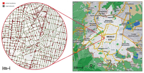
Figure 1 shows the boundary of the urban area of Mexico City (right side), as well as one street map location zoom level (left side) that allow us to perceive in detail the complexity of the city’s street network and the large numbers of criminal incidence. The streets of sample region conform a complex network of streets and avenues ranging from highways with up to 8 lanes to narrow streets that only allow pedestrian traffic. The street maps of Mexico City define a series of line segments and vertices at the intersections and consists of 229,224 vertices and 277,194 segments or edges.

Figure 1. Street network and boundary of Mexico city.

Due to the nature of the criminal activity, these occur either at points along those streets or at homes that can be assigned to a point on a threshold buffer zone for the street or avenue, which justifies the spatial analysis based on spatial point processes projected on the street network coordinate system.

However, since in point processes analysis the object of interest is the intensity function, defined as the average of events per unit area, the sub-denounce rate would only affect the magnitude, but not its shape, so descriptive inferences are valid. Based on the above discussion, the results obtained in Section 4 can be considered as scaled version of the intensity function obtained if all crimes were reported and prosecuted.

The data used in this work correspond to homicide, violent robbery and rape, reported in Mexico city for which an investigation file was opened. This implies that the events analysed are only the events that were denounced or for which the attorney’s office of Mexico City considered there were enough elements for a prosecution. It is then expected that the incidence in real terms to be greater than the one reported here. Crimes in these categories have a strong effect on society, and as a result, the government imposed a new protocol in police action since January 2018. This significant step ahead, taken in the fight against criminality, allows police officers to geo-reference any criminal incidence reported and assisted by them. As a result, a database that includes the street map, the spatial and temporal coordinates of the crimes and other relevant information is created.

Thereby, the databases are stored in the public domain of the Attorney General of Mexico City. All the denounced crimes with an investigation file between January 2018 and December 2019 are free to download after an authorization request. In this database, the total number of crimes considered for this study and prosecuted for 2018 is 53,890, while for 2019, the total crimes prosecuted is 44,344. The variables included in our study are: the geographical position in which the crime occurred, type of crime and year of occurrence.

Based on the above data, we propose to identify some pattern of crime incidence and spatial association between crime types from past case summaries and provide support to police department to identify different crime patterns and even to predict criminal activities. The results could be used in intelligent crime analysis and guide the decision-makers to increase the number of law enforcement in some areas where the prediction shows a high risk of crimes.

3. Spatial and statistical methods

Statistical data analysis comprised the use of exploratory and inferential techniques to gain insight about the spatial variation of crime incidence in the study area. Exploratory techniques include plots of the different variables from database and maps with counts of the number of crimes by street segments are used to gain insight about the presence of clustering of events and spatial variability patterns of different crime types considered in this work.

The patterns observed in such plots are tested through the computation of test statistics for clustering and uniformity using the free software R (version 4.1.2), (R Core Team, 2021) and following libraries: spatstat, sp, spdep, maptools, splacs, sp, raster, spatial, ggplot2, rgdal and RColorBrewer. We also explore spatial interactions of different crime types using spatial point process methods.

3.1. Spatial Point Processes

Spatial point process analysis is based on the assumption of the existence of a random mechanism from which a point configuration $X$ is chosen from a probability space. The probabilistic context thus allows to speak of things such as probability that the number of crimes in a given area $B$ is less than a fixed number $k,P[N_X(B)<k]$ or about the average number of crimes in that neighbourhood, $E[N_X(B)]$. In mathematical terms, $B$ is an arbitrary set inside a study area $W$, also known as the spatial window (in our case the urban area boundary of Mexico City). $N(B)$ denotes the number of points or events inside a set of measure $B$. Depending on the geometric space used, this set may be street segment of longitude equal to $B$ linear units or a circle of radius $r$ with area equal to $B$. Usually, the main objective is the estimation of the intensity function, defined as:

(1) $\lambda (s)=\underset{|ds|\to 0}{lim}\left\{\frac{E[N(ds)]}{(ds)}\right\}$(1)

where $s$ is a point inside $W$ and $ds$ is an infinitesimal circle centred in $s$.

The intensity function may be interpreted as a rate of the number of events (crimes) per street unit length. A quick estimator of the intensity function is the density estimator:

(2) $\lambda (s)=\frac{1}{nh}\sum _{i=1}^{n}K\left(\frac{s-s_i}{h}\right)$(2)

where $K$ is a kernel function, $n$ is the number of events in $W$ and $h$ is a parameter known as the band width that controls the amount of smoothing in the estimator of $\lambda (s)$. Thus, the intensity function can be considered as an indicator of the risk to be a crime victim in a given location $s$.

Another useful quantity for analysis of point patterns is Ripley’s $K$-function (Ripley, 1976, 1977):

(3) $\lambda K(r)=E[N(X\cap b(u,r))],$(3)

where $r$, denotes the distance between points in the pattern under analysis.

The $K$-function measures the average number of points inside a disc of radius $r$ centred in a point event u. If points in the pattern X are scattered completely at random inside $W$, then $K(r)=\pi r^2$. Departures from this value indicate non-random spread which may be clustered (above) or repulsive (below). When two or more point patterns are analysed, it is also useful to compute the $K$-cross function, $K_{ij}(r)$, defined as the expected number of type-$j$ points within a distance shorter than $r$ from an arbitrary type-$i$ point, standardized by the density of the point pattern $X_j$.

(4) $K_{ij}(r)=\frac{E\left[{\sum }_{j}I(||x^{(i)}-x^{(j)}||)<r\right]}{{\lambda }_j},$(4)

when points of $X_i$ do not interact with points of $X_j$, $K_{ij}(r)=\pi r^2$, and this implies that the two patterns are independent.

We computed the $K$ and the $K$-cross functions to the data for rape, homicide and violent robbery to test whether there is clustering, repulsion and interaction among the different crime types. The sample versions for the $K$-function is given by:

(5) $K_{ij}(r)=\sum _{i=1}^n\sum _{j=1}^m\frac{{\omega }_{ij}I(d_{ij}\le r)}{\lambda (s_i)\lambda (s_j)},$(5)

where ${\omega }_{ij}$ is an edge correction factor (Diggle, 2003) and $\lambda (s)$ is the intensity function evaluated at the data points. An analogous expression exists for the $K$-cross function.

3.2. Spatial point processes in street networks

The modelling process described in the previous section considers the point processes that are defined at every point inside the study area $W$. However, crimes usually occur in the city streets or inside buildings aligned along a network of streets in the urban area. Modelling crime data using a network approach requires some modifications of the theoretical context, mainly the topology in terms of distances. The clustering analysis and correlation in a network, for example, requires a measure of distance along paths in the network. A common practice is to measure Euclidean distance between events defined as the length of the shortest path between two points in the city. However, this may be inappropriate while analysing crime data on a linear network of city streets (Okabe and Sugihara 2012 [49]).

A linear network may be defined as the union $L={\cup }_{i=1}^N{l}_i$ of many line segments in the plane, all of them of the form $l_i=[u_i,v_i]=\{w:w=t_{ui}+(1-t)v_i,\text{break}0\le t\le 1\}$, where $u_i$, $v_i\in {\mathbb{R}}^2$ are the endpoints of $l_i$. We may assume that for $i\ne j$, the intersection of $l_i$ and $l_j$ is either empty or is one of the endpoints of $l_i$ or $l_j$.

A path between locations u and u $\prime$ in $L$ is a sequence $v_0,v_1,\dots ,v_m,v_{m+1}$ of the points in the network, with $v_0=u$ and $v_{m+1}=u{ }^{\mathrm{\prime }}$, so that $[v_i,v_{i+1}]$ is a subset of $L$ for each $i=0,\dots ,m$. The length of this path is

(6) $L=\sum _{i=0}^m\parallel v_i-v_{i+1}\parallel ,$(6)

where $\parallel \cdot \parallel$ denotes Euclidean distance.

The shortest-path distance $\delta SP(u,u{ }^{\mathrm{\prime }})$ between $u$ and $u{ }^{\mathrm{\prime }}$ is the minimum of the lengths of all paths between $u$ and $u{ }^{\mathrm{\prime }}$. If there are no such paths, then $\delta SP(u,u{ }^{\mathrm{\prime }})=\mathrm{\infty }$, which implies the network is not connected.

3.3. Estimates of intensity and independence diagnostics

There are several quick ways to get a non-parametric estimator of the intensity. A quick estimator of the intensity function is the density estimator. Traditional kernel estimators for two-dimensional data sets are not adequate for point patterns on a linear network as they put mass on points that by definition should have a null value for the intensity function. Also, kernel estimators based on the shortest network path between two points on the linear network are inadequate as they are severely biased (Ang, Baddeley, and Nair, 2020).

Instead, in this work, we use the kernel estimator implemented by Baddeley, Rubak, and Turner (2016), known as the equal split continuous kernel. This kernel is based on divisions of the street network in subsets with nodes having only first-order neighbours, second-order neighbours and so on. Such divisions ensure unbiasedness at the expense of computing cost.

The description of the mathematical details of this kernel estimator is beyond the scope of this work, but the interested reader is referred to Okabe, Satoh, and Sugihara (2009). The general form for a kernel estimator on a linear network is

(7) $\hat{\lambda }(s)=\sum _{i=1}^n\kappa \left(s,s_i\right)$(7)

where $\kappa$ is a kernel smoother, and unlike the kernel for two-dimensional data, $\kappa (\cdot ,\cdot )$ is a function of two points. For crime data on a linear network, the intensity function can be considered proportional to the risk of being a crime victim at a given location $s$.

A useful quantity for testing departures from homogeneity in point pattern analysis is Ripley’s $K$-function (Ripley, 1976, 1977). The $K$-function $K(r)$ is estimated by computing the number of points separated by an Euclidean distance $r$ standardized by the area of the study region $A$ divided by the square of the number of points in the observed pattern. The use of the Euclidean distance-based $K$-function on a linear network data induces false clustering detection at short distances and uniformity at large distances due to the network geometry. Adequate unbiased results are obtained using the geometrically corrected version proposed by Ang, Baddeley, and Nair (2012). For any network distance $r$ inside the network, the estimator has the form:

(8) ${\hat{K}}^L(r)=\frac{l}{n(n-1)}\sum _{i=1}^n\sum _{j\ne i}1\frac{1\{d_L(x_i,x_j\le r\}}{m(x_i,d_L(x_i,x_j))}$(8)

where $m(s,v)$ is a weighting factor equal to the number of points in the network that lie to exactly $v$ distance from location $s$. This weighting factor compensates for the network geometry and for a completely random point pattern on any network $L$ (Ang, Baddeley, and Nair, 2012) the correlated $K$-function is $K(r)=r$. Departures from this line are indicative of either clustering or repulsion between the events on the network.

We compute the $K$ and the $K$-cross functions to the data for rape, homicide and violent robbery to test whether there is clustering, repulsion and interaction among the different crime types. The sample version for the $K$-function is given by

(9) $K_{ij}(r)=\frac{1}{|L|}\sum _{x_l\in {\mathbf{X}}_i}\sum _{x_k\in {\mathbf{X}}_j}\frac{1\{d_L(x_i,x_j\le r\}}{{\hat{\lambda }}_i(x_l){\hat{\lambda }}_j(x_k)m(x_l,d_L(x_l,x_k))}$(9)

where ${\hat{\lambda }}_i$ and ${\hat{\lambda }}_j$ are estimator for the intensity function of crimes of type $i$ and $j$, respectively.

When $\lambda (s)=\lambda$ is constant, point events occur at a uniform rate in $B$ and we call this Complete Spatial Randomness (CSR) in $B$. Departures from CSR may be in the form of clustering or as repulsion among point events. Detection of such departures can be done using second-order properties of point patterns.

Tests of CSR are executed using the $K$-function whilst tests of point pattern independence for the three crime types are constructed using the cross $K$-function. Envelopes for all tests were constructed from simulations of Homogeneous Poisson Point Patterns.

Departures of the empirical $K$- or $K$-cross functions above the $\pi r^2$ line are indicative of clustering and non-independence among the crime types, respectively (Moller and Waagepetersen, 2004; Baddeley and Turner, 2005).

4. Results and discussion

Exploratory data analysis provides information about marginal correlations and possible non-spatial grouping of observations in the database. Such groups may indicate the presence of subpopulation and geographic zonation of crime occurrences in Mexico City.

The total number of occurrences for the three types of crime considered in this study is found to be nearly identical in 2018 and 2019, with only minor differences due to the random nature of crime occurrences (Table 1). The monthly incidence for each crime type shows some variations from 2018 to 2019 as follows: monthly averages from 2018 to 2019 decrease by 18.59% for violent robbery, the rape increase by 3.25%, while the homicide crime increased by one case. The overall incidence crimes for the three crime types in terms of number of events per month show a decrease of 17.71% from 2018 to 2019 in the number of investigation folders.

Table 1. Numbers of crimes reported in Mexico city for two years.

Type of crime	2018		2019
	Incidence	Inc./month	Incidence	Inc./month
Homicide	1301	108.42	1302	108.50
Violent robbery	51,544	4295.33	41,963	3496.92
Rape	1045	87.08	1079	89.92
Total	53,890	4490.83	44,344	3695.33

However, it is difficult to tell if the decrease is due to a higher number of police interventions or due to a decrease in the number of denounces. Only homicides are prosecuted without denouncement, so in this case, the increase in the number of crimes is linked to an increase in the number of events.

4.1. Spatial distribution of crime incidence

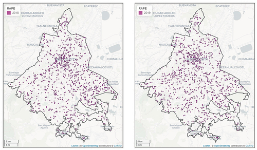
Figure 2 depicts the spatial patterns of incidents of reported rape offences with investigation files for the years 2018 (left) and 2019 (right). For this crime, the pattern of occurrences is very similar in both years. There seem to be small clusters of rape events in the ‘Historic Center’ and surrounding areas. For the rest of the city, the pattern seems to be completely random, as some small clusters are expected given the high number of events in the study area. Note the existence of aligned points in some areas of the city, which suggests the existence of streets or avenues where this type of crimes are being committed repeatedly. The absence of events in the southern part of the city is due to the fact that it is a rural area, where the population density is comparatively low compared to the rest of the urban area.

Figure 2. Reported rapes in Mexico city for 2018 (left) and 2019 (right).

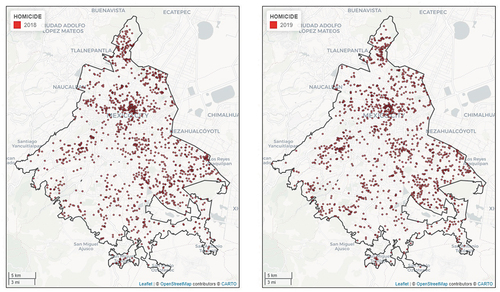
Figure 3 shows the location of the homicides that occurred in Mexico City during the years 2018 (left) and 2019 (right). The maps depict that the incidence of homicides follows the same pattern for 2018 and 2019, although the number of events has grown in 2019 and thus the size of homicide clusters has increased. The maps show the existence of areas with high incidence of homicides in the zone known as ‘Historic Center’, which comprises the oldest part of the city as well as other high murder incidence zones in the north most part of the city, in the south-west and in the south-east parts of the city. Those areas have been described as areas where drug selling gangs operate and most of the homicides are the results of fights and revenge acts among criminal groups.

Figure 3. Homicides in Mexico city.

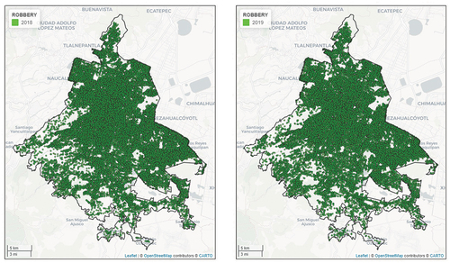
In Figure 4 we present the incidence of violent robberies in the urban area. On the left side, we report locations of violent robberies for the study year 2018, while the right side figure displays the same crime type but for the following year, 2019. As we can deduce, violent robberies are evenly spread in most part of Mexico City. The number of incidences was higher for 2018, but the spatial pattern does not show any considerable change. Basically, there is no place where a crime of this type shows lower incidence and this, in part, explains why about 37% of the population over 25 years has been the victim of a robbery at least once in their life. We can easily observe the different scale intensity due to the high number of violent robberies occurred in the same area.

Figure 4. Violent robberies in Mexico city.

The figures below this section plot the intensity functions (Kernel) for crimes studied in this article along with the spatial coordinates of points where these crimes took place. To maintain the consistency of the article, we keep the colours as in the previous figures with which we have represented for each crime type and year. The colour scale and legend used in the study are as follows: magenta for rape, red for homicide and green for violent robberies.

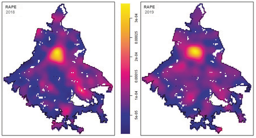
Figure 5 shows a non-parametric estimate of the intensity function (Kernel) for rape offences, considering that the specific process that generated them is defined in the Euclidean plane. The colour scale is in term of number of sexual offences per square kilometre. The estimated intensity function shows the presence of a high incidence of sexual attacks, mainly in the north of the ‘Historic Center’ (‘Barrios de La Lagunilla’, ‘Tepito’ and ‘Colonia Guerrero’) and in the ‘La Merced’ area, south-east of the ‘Zocalo’. Another peak of importance occurs in the eastern part of the City, apparently in the municipalities of ‘Iztapalapa’ and ‘Iztacalco’. The presence of three clusters aligned in a south-west direction with respect to the clusters described in the Historic Downtown area of the city is striking. These clusters occur in the area of ‘Chapultepec’, first, second and third section.

Figure 5. Intensity function for rape offences.

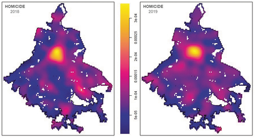
The estimate of the non-parametric intensity (Kernel) function for the homicides is shown in Figure 6. Clusters can be seen in various areas of the city, which have been considered violent neighbourhoods for several years, including the area known as ‘Tepito’, north of the ‘Historic Center’, as well as in several neighbourhoods in the municipalities of ‘Iztapalapa’ and ‘Iztacalco’ in the east, and ‘Gustavo A. Madero’ in the northern part of the city. It is not clear whether those conglomerates are associated with the high presence of drug trafficking activities and poverty in those areas, so formal statistical models for this crime type are needed. The peaks in the estimates of the intensity function make clear that intentional homicides do not occur at random in the urban area of Mexico City.

Figure 6. Kernel density estimation for homicides 2018 (left) and 2019 (right).

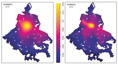
The intensity function estimate for violent robberies in Figure 7 shows that although occurrence of this type of crime is spread all over the urban area, there are wide areas where the density of robberies is very high. Those high-density zones are located in parts of the city with high economic activity (restaurants, convenience stores, banks, offices, etc.) as well as zones with industries and poor neighbourhoods. The pattern of this crime type is preserved from 2018 to 2019, despite the fact that for the last year the numbers of occurrence are reduced. This suggests that people who perpetrate this crime type have a pattern that does not change over time and that could be associated to social and economic factors that remain constant in the urban area during the study period.

Figure 7. Intensity function for violent robberies.

4.2. Spatial association between crime types

The possible spatial association between the three different crime types considered in this work was assessed using the $K$-cross function. This function measures, for a given crime type $A$ and distant $r$, the number of events of another crime type $B$ inside a circle of radius $r$ centred at an event of type $A$. If crimes of type $A$ and $B$ occur independent of each other, the $K$-cross function should follow the parabola $\pi r^2$.

In Figure 8, we plot in solid line the empirical K-cross function between crimes for 2018 with distance less than 600 metres, as well as the Monte Carlo 95% confidence for the null hypothesis of spatial independence. The dotted lines correspond to the edge corrected theoretical values for $K$-cross. The top row of the figure above displays from left to right the $K$-cross function between rape and homicides, homicides and robberies as well between robberies and rape, which occurred in 2018. Except for the rape-homicide association in 2018, the plots show strong departures from the spatial independence hypothesis, with all the empirical values above the confidence band. This implies that given that a rape has occurred at some location, one should expect a higher occurrence of homicides in a neighbourhood of radius $r$ compared to the number of homicides occurring by chance.

Figure 8. $K$-cross association function between different type of crimes and years.

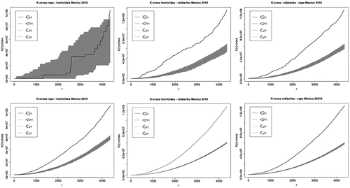
Similar conclusions can be drawn from the $K$-cross function between violent robberies and rape for the two years considered in this analysis, shown in the bottom line of the same figure. Additionally, given that a rape event has occurred at a given location, one should expect a higher occurrence of violent robberies in a neighbourhood of radius $r$. In all cases, the cluster association is shown; the black line of empirical model is always over the envelopes. Only in the first case, rape–homicides in 2018 is lined inside the envelopes. In this figure, the cluster relation for all cases is clear and it appears in full range of r. In conclusion, it can be stated that all the cross association between crime types follow same behaviour except between rape and homicide in 2018.

4.3. Application on the street network

The majority of crimes in Mexico City occur in the urban area. Moreover, the police or agents of the public prosecutor’s office associate each event to a point on a road when geo-referencing the events. As a result, the analysis of the city’s criminal incidence can be performed by considering the events as realizations of point processes defined in a street network.

The database used in this project includes the street map of the urban area of the city. Thus, through an analysis and processing of the basic information, we are able to associate the spatial coordinates of the crime events on the street map for Mexico City, projected on the same coordinate system. The street network for Mexico City is defined by a large number of line segments and the intersection nodes of the same. Although it is not possible to appreciate patterns on this map due to the large number of points, the coincidence of points and roads can be seen in areas with low crime incidence.

The process to obtain non-parametric estimates for the intensity over the network for crimes requires the computation of distances between events. Unlike the Euclidean analysis of the previous section where distance is measured as the shortest path between two points, in a linear network, distance is measured as the shortest path along the streets.

The total number of three observed types of crime in the database was 98,234. In the first step of this network-based analysis, we proceed to calculate the network distance between each incident and the others, which is 98,233. Once these distances have been computed, the second step was to calculate the kernel estimates for the intensity function along the street network.

The graphs below display only the kernel intensity function of registered crime occurrence in 2018 and 2019 over street network, but without the spatial coordinates of incidence points. As in the previous intensity function graphs, we maintain the same scales in both maps 2018 and 2019, respectively.

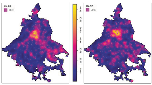
In Figure 9, we depict the density maps corresponding to rape offences over the street network for 2018 (left) and 2019 (right). According to these maps, in 2018, this kind of crime is concentrated in the central and eastern region of the urban area.

Figure 9. Network intensity function for rapes in Mexico city.

For 2019, sexual attacks were concentrated around the same high-density zone of 2018, but spread south and north-east sides of it. It is noteworthy that some peaks have been identified in the western boundaries of the city and others in the south-east in 2019. Nevertheless, the maps show that the geographic pattern for this crime has changed. In both years, the figure suggests the presence of some degree of clustering.

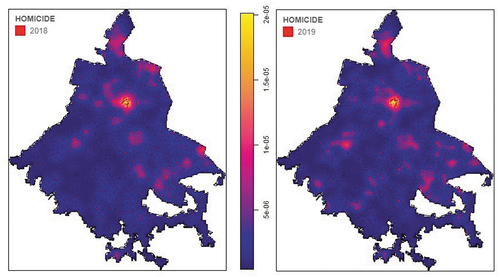
Figure 10 shows the intensity maps for intentional homicides for the two years considered in the analysis. Homicides in 2018 showed a high-intensity zone in the area around the ‘Historic Center’. This area contains several buildings inhabited by poor families and is the area where two of the most conflictive neighbourhoods (‘Tepito’ and ‘Colonia Morelos’) are located. Other areas of high homicide incidence are located in the north, north-east, south-east and southern parts of the city.

Figure 10. Network intensity function for homicides 2018 (left) and 2019 (right).

The map for 2019 shows the same high-intensity spot around the city centre. The other high-density spots seem to have increased in intensity. Homicides in Mexico city may occur anywhere, but the previous maps highlight the presence of zones where this kind of crime has higher incidence as compared to other areas of the city. It is not clear why this high incidence is observed in some zones, but most of them coincide with poor neighbourhoods and areas where drug traffic activities have been reported.

Thus, the kernel estimate of the intensity function only has small peaks that could be analysed separately defining a small region of interest in such a way that only includes the cluster of interest in the map.

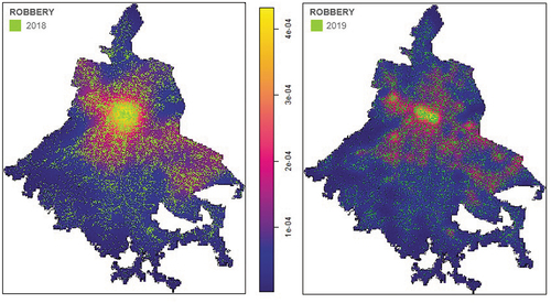
Figure 11 represents the intensity function over streets network of violent robberies that befell in 2018 (left) and 2019 (right). The pattern is similar to the rape offences, but on a lower intensity scale. It seems that violent robberies are met close or around the high-density zone of rape activity described in Figure 9.

Figure 11. Violent robberies intensity function over network.

For dataset of 2018, the streets network of Mexico City downtown is completely covered by the highest intensity of violent robberies. The intensity is highly concentrated in the ‘Historic Center’, as this is the area with a high concentration of stores, office and commercial activity and the number of potential victims is higher than in other parts of the city. While for 2019 the higher intensity increases in the same area, the pattern of violent robberies shows the intensity function has spread over a wider region of the city, mainly in the north-west.

We remarked a significant scaling down of violent robberies in downtown city. Note that the values of the scale for the estimated intensity function for 2019 are about three-quarters of the values for 2018. The significant decrease of intensity crimes cluster in the city centre could be explained by the police actions in this area.

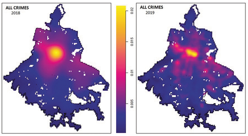
Figure 12 shows the kernel estimate of the intensity function over street network computed using the locations of all the crime types for the two years. This map depicts the locations of the city with the highest levels of criminality, independent of the type of crime. The map shows that criminal incidents tend to occur around a high-intensity zone that runs east to west along the urban area. This zone covers parts of Mexico City that have a large history of criminal activity and where social factors contribute to the high incidence of crimes. The map also shows that crime activity spreads north and south of the high-intensity zone, mainly to areas where crimes like violent robbery are profitable for criminals.

Figure 12. All crimes kernel intensity function in 2018 (left) and 2019 (right).

The data analysed in this work showed that crime occur in clusters in the study area, with higher incidence of homicide in the old part of the city. The overall spatial pattern (the three crime types together) of crime occurrences in Mexico City is similar for 2018 and 2019, despite the lower crime incidence in the final study year. The number of crimes decreased in 2019 as compared to the number for 2018. The maps for both years highlight the same areas of high crime incidence. It is not clear if such reduction was the result of new public safety strategies of the new administration in the government, or if such reduction in crime incidence was associated with a reduction in the number of investigation folders.

5. Conclusions

Criminal incidence in Mexico City is high, and the population’s perception of insecurity is that criminal activities may occur practically anywhere in the urban area. Therefore, crime in Mexico City is a deep concern for the working population and for the government. Except for homicides that are prosecuted ex-officium, it is believed that a high proportion of other crimes and offences are not denounced either because of a lack of trust in the justice system or because of the fear of the burden that following a denounce implies in Mexico. The amount of unreported crimes, on the other hand, makes it difficult to evaluate more reliable quantities, such as the relative risk for each crime type, because these quantities require knowledge of the total number of crimes committed in the city.

A person who is the victim of a crime in Mexico City does not go to the authorities to make a denounce. Thus, only a fraction of those denounces passes to the stage of ‘investigation file’, either because the victim decides not to keep the legal process or because there are not enough proofs against the criminals, so the data analysed here are only a small fraction of the real number of crimes.

Nevertheless, we assumed that the observed spatial point pattern for the three crime types is a randomly thinned version of the true pattern. Thinning of point processes preserves the spatial properties of the original point process (Karr, 1986); thus, our results are still useful for potential users, such as law enforcement agencies, researchers and general public.

The advantage of the analysis of crime incidence using spatial point patterns is that it permits to obtain good estimates of the actual pattern of crime incidence, despite the low number of denounces. Such estimates are a surrogate of the true crime incidence in the street network, follow closely the pattern of the risk of becoming a victim of a given crime type. Note that the estimates obtained in this work do not aim at explaining the causes of crime incidence in Mexico City, but only to provide a method to obtain spatial incidence maps that can be used by authorities and the general public.

Spatial point processes are a powerful and useful tool for the analysis of criminality in geographic areas. This tool is also useful to detect hot spots and with appropriate modelling, it can be used to predict future trends in crime incidence. Although modelling requires advanced training in statistics, analysis such as the one we have presented in this work can be done using standard statistical and geo-spatial tools.

The use of point pattern analysis techniques allows detecting in a non-subjective way the areas of higher crime incidence. There are differences in the results computed when kernel estimation of the intensity function is obtained using Euclidean distance and network distance. Those differences are explained by stronger smoothing induced by kernel based on Euclidean distance as this approach assigns density to locations out of the street network.

The spatial analysis of crime incidence we have done on a linear network allows us to identify street segments where the incidence is higher than in neighbouring street segments. This information is potentially useful for authorities as high incidence in some streets may be indicative of the existence of crime gangs operating in those particular streets.

The $K$-cross analysis of the three crime types has shown that they are independent of each other. It indicates that the intensity of a given crime type does not affect the incidence rate of the other two. This is an important result, as it suggests that different risk variables may influence the three categories of crime studied.

Rape offences occur with similar intensity in Mexico City in both years, with the higher intensity in the ‘Historic Center’ zone (‘La Lagunilla’, ‘Tepito’ and ‘Colonia Morelos’ neighbourhoods) and a high number of small clusters scattered all over the city’s urban area. This area, known as ‘Historic Center’, is an area with a high density of commerce and offices that attracts a high number of potential crime victims. This high incidence is also promoted by the high density of non-formal commerce in the street that helps criminals to hide and escape by blending in the crowd (Adel, Salheen, and Mahmoud, 2016). The numerous old buildings in this area known as ‘vecindades’ also provide refuge for crime perpetrators, who most of the time are protected by their neighbours and relatives who block police action. Rapes have been associated to familiarity between the victim and the perpetrator, and that is a risk factor (Boggs, 1965). This may explain, in part, why the spatial incidence of this crime type is clustered on poor areas of the city and the ‘Historic Center’. Rape offences occur in almost all the urban area, but some areas have higher incidence. Most of these clusters are located in the South East part of the city, in the municipalities of ‘Iztapalapa’ and ‘Tlahuac’.

Homicides are also concentrated in the area of the ‘Historic Center’, but several other clusters were detected in territories of the municipalities of ‘Alvaro Obregón’ in the West, ‘Gustavo A. Madero’ in the North and in the South East, in the ‘Iztapalapa’ and ‘Tlahuac’ municipalities. This pattern is similar during 2018 and 2019. As we saw, a higher occurrence of homicides could appear in the clusters associated with rapes. These clusters were associated with poor neighbourhood zones and traffic dealer activities.

Violent robberies have a similar spatial pattern in both years, but the decrease in the number of this crime type from 2018 to 2019 results in the apparent presence of some degree of clustering during 2019. Robberies occur in all the urban areas, but some areas have higher incidence, such us ‘Historic Center’. The connectivity that the street network of the city provides gives escape routes to robbers. Because such connectivity exists in all the urban areas, violent robberies may occur anywhere in the city. Another reason for high robbery incidence is because many cases of murder and rape have been reported together with the theft of the victim’s goods. The $K$-cross association between homicide–robberies and robbery–rape also explains why so many thefts are recorded in Mexico City.

Our analysis has shown that the three crime types considered in this study are not independent pairwise and the spatial distribution is in a clustered pattern, concentrated in the area known as ‘Historic Center’. Also, that individual crime types have a distinct spatial distribution and rape and homicide are spatially associated, although they do not necessarily occur simultaneously. A possible explanation is that crimes are more frequent in areas with a high density of commercial and administrative activity where the density of possible victims is higher.

Therefore, the maps obtained in this study can be used to design strategies for crime prevention and combat. It is clear that although the government of Mexico City has claimed that high numbers of crime incidences are non-significant, the non-parametric estimates obtained on the street network clearly show the existence of areas in the city where the chances of becoming a victim of a crime are higher than in others.

Despite minor changes in the spatial pattern of crime incidence in Mexico City, the overall number of crimes between 2018 and 2019 has not changed significantly. The areas with a high crime incidence have remained unchanged, implying that the current local authorities’ efforts to combat crime require strategic improvement. According to our findings, the attempts have worked properly in the case of violent robberies.

Using external information for social and economic variables, point pattern analysis can be used to screen out which factors influence crime incidence and if the effect of those variables shows spatial variation. The inclusion of external variables on point process analysis and inference has been described by Baddeley, Rubak, and Turner (2016) and Diggle (2003), among others.

Further research is required to detect social, economic and urban architecture factors that might explain the clustering of crimes, mainly rape and homicides in some parts of Mexico City’s urban area. This analysis can be done using spatial point processes on linear networks at street spatial resolution, provided adequate data exist.

Disclosure statement

No potential conflict of interest was reported by the authors.

Additional information

Funding

This work was supported by the Carlos Díaz-Avalos was supported by PAPIIT-DGAPA project number IG100221 [IG100221].

References

- Adams, W., C. Herrmann, and M. Felson. 2015. “Crime, Transportation and Malignant Mixes.” In Safety and Security in Transit Environments: An Interdisciplinary Perspective, edited by V. Ceccato and A. Newton, 181–195. Basingstoke, Hampshire: Palgrave McMillan.
- Adel, H., M. Salheen, and R. A. Mahmoud. 2016. “Crime in Relation to Urban Design. Case Study: The Greater Cairo Region.” Ain Shams Engineering Journal 7 (3): 925–938. doi:10.1016/j.asej.2015.08.009.
- Andersen, M. 2006. “A Spatial Analysis of Crime in Vancouver, British Columbia: A Synthesis of Social Disorganization and Routine Activity Theory.” The Canadian Geographer 50 (4): 487–502. doi:10.1111/j.1541-0064.2006.00159.x.
- Andresen, M. A., and T. Hodgkinson. 2018. “Predicting Property Crime Risk: An Application of Risk Terrain Modeling in Vancouver, Canada.” European Journal on Criminal Policy and Research 24 (4): 373–392. doi:10.1007/s10610-018-9386-1.
- Andresen, M. A., Linning, N. Malleson, and S. J. Linning. 2017. “Crime at Places and Spatial Concentrations: Exploring the Spatial Stability of Property Crime in Vancouver BC, 2003–2013.” Journal of Quantitative Criminology 33 (2): 1–21. doi:10.1007/s10940-016-9295-8.
- Ang, Q. W., A. Baddeley, and G. Nair. 2012. “Geometrically Corrected Second Order Analysis of Events on a Linear Network, with Applications to Ecology and Criminology.” Scandinavian Journal of Statistics 39 (4): 591–617. doi:10.1111/j.1467-9469.2011.00752.x.
- Baddeley, A. 2006. Case Studies in Spatial Point Process Modeling. Springer-Verlag New York, Springer. https://doi.org/10.1007/0-387-31144-0
- Baddeley, A. 2010. Multivariate and Marked Point Processes. in P Guttorp (ed.), Handbook of Spatial Statistics. Handbooks of Modern Statistical Methods, Chapman & Hall/CRC Press, Boca Raton, USA, pp 371–402.
- Baddeley, A., J. Møller, and R. Waagepetersen. 2000. “Non and semi-parametric Estimation of Interaction in Inhomogeneous Point Patterns.” Statistica Neerlandica 54 (3): 329–350. doi:10.1111/1467-9574.00144.
- Baddeley, A., G. Nair, S. Rakshit, G. McSwiggan, and T. M. Davies. 2020. Analysing Point Patterns on Networks – A Review. Spatial Statistics. 100435. doi:10.1016/j.spasta.2020.100435.
- Baddeley, A., E. Rubak, and R. Turner. 2016. Spatial Point Patterns. Methodology and Applications with R. N. Y: Chapman and Hall.
- Baddeley, A., and R. Turner. 2005. “Spatstat: An R Package for Analyzing Spatial Point Patterns.” Journal of Statistical Software ch 12 (6): 195–217. doi:10.18637/jss.v012.i06.
- Boggs, S. L. 1965. “Urban Crime Patterns.” American Sociological Review 30 (6): 899–908. doi:10.2307/2090968.
- Bowers, K. J., and S. D. Johnson. 2003. “Measuring the Geographical Displacement and Diffusion of Benefit Effects of Crime Prevention Activity.” Journal of Quantitative Criminology 19 (3): 275–301. doi:10.1023/A:1024909009240.
- Braga, A. A., A. V. Papachristos, and D. M. Hureau. 2014. “The Effects of Hot Spots Policing on Crime: An Updated Systematic Review and meta-analysis.” Justice Quarterly 31 (4): 633–663. doi:10.1080/07418825.2012.673632.
- Brillinger, D. R., H. K. Preisler, and J. W. Benoit. 2003. “Risk Assessment: A Forest Fire Example.” Lecture Notes-Monograph Series 177–196.
- Butt, U. M., S. Letchmunan, F. H. Hassan, M. Ali, A. Baqir, and H. H. R. Sherazi. 2020. “Spatio-Temporal Crime HotSpot Detection and Prediction: A Systematic Literature Review.” IEEE Access 8: 166553–166574. doi:10.1109/ACCESS.2020.3022808.
- Caplan, J. M., L. W. Kennedy, E. L. Piza, and J. D. Barnum. 2020. “Using Vulnerability and Exposure to Improve Robbery Prediction and Target Area Selection.” Applied Spatial Analysis and Policy 13 (1): 113–136. doi:10.1007/s12061-019-09294-7.
- Chainey, S., and J. Ratcliffe. 2005. GIS and Crime Mapping. New York: Wiley.
- Connealy, N. T., and E. L. Piza. 2019. “Risk Factor and high-risk Place Variations across Different Robbery Targets in Denver Colorado.” Journal of Criminal Justice 60: 47–56. doi:10.1016/j.jcrimjus.2018.11.003.
- Daley, D. J., and D. Vere-Jones. 2003. An Introduction to the Theory of Point Processes. Vol. I. 2nd ed ed. Springer, New York: Elementary Theory and Methods.
- Daley, D. J., and D. Vere-Jones. 2008. “An Introduction to the Theory of Point Processes.” 2nd ed. Volume II: General Theory and Structure. 157-210. New York: Springer.
- Díaz-Avalos, C., P. Juan, and L. Serra-Saurina. 2016. “Modeling Fire Size of Wildfires in Castellon (Spain), Using Spatiotemporal Marked Point Processes.” Forest Ecology and Management 381: 360–369. doi:10.1016/j.foreco.2016.09.013.
- Diggle, P. 1979. “On Parameter Estimation and goodness-of-fit Testing for Spatial Point Patterns.” Biometrics 35 (1): 87–101. doi:10.2307/2529938.
- Diggle, P. J. 2003. Statistical Analysis of Spatial Point Patterns. 2nd Edition ed. London: Arnold.
- Dixon, P. M., A. H. El-Shaarawi, and W. Piegorsch. 2012. “Ripley’s K Function.” Encyclopedia of Environmetrics 3.
- Drawve, G., S. C. Moak, and E. R. Berthelot. 2016. “Predictability of Gun Crimes: A Comparison of Hot Spot and Risk Terrain Modelling Techniques.” Policing and Society 26 (3): 312–331. doi:10.1080/10439463.2014.942851.
- Gelfand, A. E., P. Diggle, P. Guttorp, and M. Fuentes. 2010. Handbook of Spatial Statistics. CRC press.
- González Andrade, S. 2014. “Criminality and Regional Economic Growth in Mexico.” Frontera Norte 26 (51): 75–111. 2594-0260.
- Gonzalez, J. A., F. J. Rodriguez-Cortes, O. Cronie, and J. Mateu. 2016. “Spatio-temporal Point Process Statistics: A Review.” Spatial Statistics 18: 505–544. doi:10.1016/j.spasta.2016.10.002.
- Grubesic, T. H., and W. A. Pridemore. 2011. “Alcohol Outlets and Clusters of Violence.” International Journal of Health Geographics 10 (1): 30. Article 30. doi:10.1186/1476-072X-10-30.
- INEGI 2020. “Census of Population and Housing Units.” Webpage: http://www.inegi.org.mx/programas/ccpv/2020
- Jiang, C., L. Liu, X. Qin, S. Zhou, and K. Liu. 2021. “Discovering Spatial-Temporal Indication of Crime Association (STICA).” ISPRS International Journal of Geo-Information 10 (2): 67. MDPI AG. Retrieved from. doi:10.3390/ijgi10020067.
- Jiménez, R. A. 2003. “La cifra negra de la delincuencia en México: Sistema de encuestas sobre victimización.” In Proyectos legislativos y otros temas penales. Segundas jornadas sobre justicia penal, México, Instituto de Investigaciones Jurídicas, edited by S. García Ramírez Y and L. A. Vargas Casillas. Mexic.
- Johnson, S. D., R. T. Guerette, and K. J. Bowers. 2014. “Crime Displacement: What We Know, What We Don’t Know, and What It Means for Crime Reduction.” Journal of Experimental Criminology 10 (4): 549–571. doi:10.1007/s11292-014-9209-4.
- Juan, P., J. Mateu, and M. Saez. 2012. “Pinpointing spatio-temporal Interactions in Wildfire Patterns.” Stochastic Environmental Research and Risk Assessment 26 (8): 1131–1150. doi:10.1007/s00477-012-0568-y.
- Karr, A. F. 1986. Point Processes and Their Statistical Inference. New York and Basel: Marcel Dekker.
- Leong, K., and A. Sung. 2015. “A Review of spatio-temporal Pattern Analysis Approaches on Crime Analysis.” Int. e-J. Crim. Sci 9: 1.
- Levine, N. 2015. CrimeStat: A Spatial Statistics Program for the Analysis of Crime Incident Locations (V 4.02). Washington DC: Levine, Houston, and National Institute of Justice.
- Mohler, G. O. 2014. “Marked Point Process Hotspot Maps for Homicide and Gun Crime Prediction in Chicago.” International Journal of Forecasting 30 (3): 491–497. doi:10.1016/j.ijforecast.2014.01.004.
- Mohler, G. O., M. B. Short, P. J. Brantingham, F. P. Schoenberg, and G. E. Tita. 2011. “Self-exciting Point Process Modeling of Crime.” Journal of the American Statistical Association 106 (493): 100–108. doi:10.1198/jasa.2011.ap09546.
- Møller, J., and C. Díaz-Avalos. 2010. “Structured spatio-temporal shot-noise Cox Point Process Models, with a View to Modelling Forest Fires.” Scandinavian Journal of Statistics 37 (1): 2–25. doi:10.1111/j.1467-9469.2009.00670.x.
- Moller, J., and R. P. Waagepetersen. 2004. Statistical Inference and Simulation for Spatial Point Processes. New York: CRC Press.
- Newton, A., and M. Felson. 2015. “Crime Patterns in Time and Space: The Dynamics of Crime Opportunities in Urban Areas.” Crime Science 4 (1): 11. doi:10.1186/s40163-015-0025-6.
- Newton, A., and A. Hirschfield. 2009. “Measuring Violence in and around Licensed Premises: The Need for a Better Evidence Base.” Crime Prevention and Community Safety. An International Journal 11 (3): 171–188. doi:10.1057/cpcs.2009.12.
- Ogata, Y. 2011. “Significant Improvements of the space-time ETAS Model for Forecasting of Accurate Baseline Seismicity.” Earth, Planets and Space 63 (3): 217–229. doi:10.5047/eps.2010.09.001.
- Ogata, Y., and M. Tanemura. 1981. “Estimation of Interaction Potentials of Spatial Point Patterns through the Maximum Likelihood Procedure.” Annals of the Institute of Statistical Mathematics 33 (2): 315–338.
- Okabe, A., T. Satoh, and K. Sugihara. 2009. “A Kernel Density Estimation Method for Networks, Its Computational Method and A GIS-Based Tool.” International Journal of Geographical Information Science 23 (1): 7–32. doi:10.1080/13658810802475491.
- Okabe, A., and K. Sugihara. 2012. Spatial Analysis along Networks: Statistical and Computational Methods. New York: John Wiley & Sons.
- Opitz, T., F. Bonneu, and E. Gabriel. 2020. “Point-process Based Bayesian Modeling of space–time Structures of Forest Fire Occurrences in Mediterranean France.” Spatial Statistics 40: 100429. doi:10.1016/j.spasta.2020.100429.
- Pansters, W., and B. H. Castíllo. 2007. “Violencia e inseguridad en la ciudad de México: Entre la fragmentación y la politización”. Foro Internacional. XLVII:577–615. 0185-013X. URL. https://www.redalyc.org/articulo.oa?id=59911150005
- Quick, M., L. Guangquan, Ian Brunton-Smith, and I. Brunton-Smith. 2018. “Crime-general and crime-specific Spatial Patterns: A Multivariate Spatial Analysis of Four Crime Types at the small-area Scale.” Journal of Criminal Justice 58: 22–32. doi:10.1016/j.jcrimjus.2018.06.003.
- R Core Team. 2021. R: A Language and Environment for Statistical Computing. Vienna, Austria: R Foundation for Statistical Computing. https://www.R-project.org/
- Reinhart, A. 2018. “Point Process Modeling with Spatiotemporal Covariates for Predicting Crime. Carnegie Mellon University.” Thesis. doi:10.1184/R1/7178903.v1.
- Reinhart, A., and J. Greenhouse. 2018. “Self-exciting Point Processes with Spatial Covariates: Modelling the Dynamics of Crime.” Journal of the Royal Statistical Society 67 (5): 1305–1329. Series C (Applied Statistics).
- Ripley, B. D. 1976. “The second-order Analysis of Stationary Point Processes.” Journal of Applied Probability. ch 13. 256–266.
- Ripley, B. D. 1977. “Modelling Spatial Patterns.” Journal of the Royal Statistical Society, Series B 39: 172–212.
- Tao, R., and J. C. Thill. 2019. “Flow Cross K-function: A Bivariate Flow Analytical Method.” International Journal of Geographical Information Science 33 (10): 2055–2071. doi:10.1080/13658816.2019.1608362.
- Van Lieshout, M. N. M., and A. Baddeley. 1999. “Indices of Dependence between Types in Multivariate Point Patterns.” Scandinavian Journal of Statistics 26 (4): 511–532. doi:10.1111/1467-9469.00165.
- Vilalta, C., and R. Muggah. 2016. “What Explains Criminal Violence in Mexico City? A Test of Two Theories of Crime.” Stability: International Journal of Security and Development 5 (1): 1–22. doi:10.5334/sta.433.
- Waagepetersen, R., Y. Guan, A. Jalilian, and J. Mateu. 2016. “Analysis of Multispecies Point Patterns by Using Multivariate log-Gaussian Cox Processes.” Journal of the Royal Statistical Society 65 (1): 77–96. Series C (Applied Statistics).
- Wang, Z. Temporal-Spatial Hot Spot Analysis on Crime Cases Based on Scan Statistics Methodologies in Shanghai. Ph.D. Thesis, East China Normal University, Shanghai, China, 2013.
- Wang, L., G. Lee, and I. Williams. 2019. “The Spatial and Social Patterning of Property and Violent Crime in Toronto Neighbourhoods.” A spatial-quantitative Approach 8. doi:10.3390/ijgi8010051.
- Wang, Z., L. Liu, H. Zhou, and M. Lan. 2019. “Crime Geographical Displacement: Testing Its Potential Contribution to Crime Prediction.” ISPRS International Journal of Geo-Information 8 (9): 383. doi:10.3390/ijgi8090383.
- Weisburd, D., W. Bernasco, and G. J. N. Bruinsma. 2009. “Units of Analysis in Geographic Criminology: Historical Development,critical Issues, and Open Questions.” In Putting Crime in Its Place: Units of Analysis in Geographic Criminology, edited by D. Weisburd, W. Bernasco, and G. J. N. Bruinsma. New York: Springer.