Application of GIS and fuzzy sets to small-scale site suitability assessment for extensive brackish water aquaculture

ABSTRACT

The rapid expansion of extensive brackish water aquaculture (BA) in Indonesia has created an urgent need to develop effective and reliable methods to evaluate and select sites suitable for aquaculture development. The lack of supporting spatial data at appropriate scales has limited the application of GIS-based multi-criteria evaluation methods (MCEs) in Indonesia. This study presents alternative fuzzy-based Geographic Information System (GIS) methods to evaluate and select sites suitable for extensive brackish water aquaculture. This study successfully produced fuzzy set maps from a water availability sub-model, a land conversion sub-model and a green belt buffer zone sub-model. With grades of membership, the fuzzy set maps provide smooth class boundary representation, which creates more options for decision-making than a map classified with crisp logic. Combining these sub-models produced an overall site suitability map at the scale of 1:50,000 for the study region. This final suitability map effectively excluded more than 95% of the unsuitable area for BA. This broad-scale site suitability assessment approach is a helpful planning tool to promote Indonesia’s sustainable development of extensive brackish water aquaculture. It identifies possible conflicts in land uses and considers conservation issues early in the planning process. The output can be used to scope research areas for more detailed investigations in countries where BA is a vital livelihood.

KEYWORDS:

• Site assessment
• aquaculture
• fuzzy set
• GIS

1. Introduction

Aquaculture is economically and socially important to people in many developing countries, including Indonesia. It contributes to national food security, income, employment generation and foreign exchange earnings. In recent years, aquaculture has also been considered a means to reduce pressure on marine natural resources through its role as an alternative source of income for coastal fishery communities (Ateweberhan et al. 2018). Indonesia has great potential for aquaculture as the country comprises 17,504 islands and has a coastline of around 108,000 kilometres accounting for 14% of the world’s coastline (MMAF 2019). Aquaculture in Indonesia is practiced in marine, brackish and freshwater with various species, production systems and methods. There are an estimated 2,964,331 hectares (ha) with the potential for brackish water aquaculture, but only 650,509 (21.9%) ha were in operation in 2018, with an annual production of 1.6 million metric tonnes (MMAF 2019). The traditional low-density earthen coastal aquaculture, also called an extensive system, remains dominant in Indonesia because it provides food security for smallholder farmers. The more intensive farms are unsustainable; they require significant inputs of chemicals and face high on-farm risks from disease, self-pollution and other impacts from adjoining farms (Hanafi and Ahmad 1996; Kusumastanto, Jolly, and Bailey 1998; Macusi et al. 2022; Rubel et al. 2019).

The lack of proper site selection criteria and land capability schemes has been identified as one of the primary reasons for the failure of most extensive brackish water aquaculture in Southeast Asia, particularly in Indonesia (Anand et al. 2021; Poernomo 1992; White, Phillips, and Beveridge 2013). The signs of poor site selection are evident with many existing ponds built in unsuitable locations, including coastal areas associated with acid sulphate soils, areas above the mean highest tide level, buffer zone conservation areas and locations previously used for productive agriculture systems (e.g. rice field) (Bagarinao and Primavera 2005; Karstens and Lukas 2014; Tarunamulia and Sammut 2022). This haphazard land development of aquaculture fails to achieve adequate productivity and seriously threatens nearby ecosystems and neighbouring land uses. One of the most urgent tasks is to provide spatial information support tools and mechanisms to help reduce the rate of pond expansion in unsuitable locations, especially the development of pond areas that convert mangrove conservation areas.

Previous studies demonstrated the advantages and potential applications of Geographical Information Systems (GIS) and remote sensing to improve the quality of mapping methods and related outputs for aquaculture planning and management (Falconer et al. 2017, 2020; Giap, Yi, and Yakupitiyage 2005; Gimpel et al. 2018; González-Rivas and Tapia-Silva 2023; Jayanthi et al. 2006, 2018; Salam, Khatun, and Ali 2005; Silva et al. 2011; Wanchana and Sayan 2018; Wang et al. 2022). In general, GIS provides spatial decision support for site assessment (Falconer et al. 2017), sustainable management and monitoring aquaculture land-use changes (Diep et al. 2019; Longdill, Healy, and Black 2008), and to assess and predict environmental impacts (Jayanthi et al. 2018; Nagamani and Suresh 2019; Panchatcharam and Anand 2017; Pérez et al. 2003; Radiarta, Saitoh, and Miyazono 2008). Most past studies appreciated the application of GIS techniques to aquaculture site selection processes due to the ability to integrate multiple variables or factors during analysis (Bandira et al. 2021; Giap, Yi, and Yakupitiyage 2005; Rajitha, Mukherjee, and Vinu Chandran 2007; Salam, Khatun, and Ali 2005). Interestingly, although most studies list several variables utilized in their study, the final classification is often dictated by limited thematic maps such as maps of mudflats, land use and landform classification as a starting point (Giap, Yi, and Yakupitiyage 2005; Karthik et al. 2005; Rajitha, Mukherjee, and Vinu Chandran 2007). Other variables were used only to score or weight the pre-defined classes. Recent studies have tried to combine multiple thematic maps to produce a final land suitability map (Ghobadi, Nasri, and Ahmadipari 2021; Jayanthi et al. 2020; Nayak et al. 2018; Nguyen et al. 2022); however, the process and results may be criticized for weighting and combining variables that should not be equal such as water quality versus infrastructure. The score assignment of the multiple layers was usually performed by Saaty’s Analytical Hierarchy Process (AHP) method requiring subjective expert judgement (Nguyen et al. 2022). In such a situation, where qualitative data and human expertise are integrated into the modelling, the fuzzy set method (Zadeh 1999) plays a key role in modelling the fuzziness of the human cognitive processes such that suitability classes do not have sharp or crisp boundaries but degrees of membership between classes (Bórquez-Lopez et al. 2018; Carbajal-Hernández et al. 2012).

There are some existing technical or practical issues in GIS-based spatial analysis, such as the availability of supporting geospatial data and accuracy assessment (Huang, Cao, and Silva 2017; Silva et al. 2011; Wong and Lee 2005). The geographical data (spatial and tabular data) used in the GIS analysis come from various sources, ages, levels of detail and position accuracy (Huang, Cao, and Silva 2017; Kapetsky, McGregor, and Nanne 1987; Thapa and Bossler 1992). Consequently, there is uncertainty regarding the accuracy of the results and applications. In most developing countries, it is unlikely to find coastal areas within a specific administrative boundary with complete geospatial datasets for all key environmental variables. Because of that limitation, it is necessary to develop a method that accounts for incomplete geospatial datasets without diminishing the objectiveness and accuracy of the analysis. Accordingly, the selection of key variables provides a solution for the initial planning site assessment and compensates for the unavailability of geospatial data.

This study aims to apply fuzzy set techniques in the GIS environment to improve small-scale site suitability assessment of brackish water aquaculture. The selection of key environmental factors is intended to improve time and cost-efficiency and to promote practicality in the analysis. Integrating a fuzzy set-based GIS approach to deal with BA environmental factors may improve spatial decision tools.

2. Materials and methods

2.1. The study site

This study used spatial datasets from the coastal areas of Barru District, South Sulawesi, Indonesia (Figure 1). The existing brackish water ponds, which are predominantly extensive farms, cover an area of about 16 km². Extensive ponds are generally less than 2 ha and are based on low shrimp stocking densities and minimal farm inputs (Hanafi and Ahmad 1996; Kusumastanto, Jolly, and Bailey 1998). They also depend on tidal exchange to supply and remove water; consequently, extensive farms are restricted to the coastal lowlands. The study site is located between latitude 4° 12’ 23” and 4° 29’ 50” S and stretches between 119° 35’ 32” and 119° 39’ 08” E longitudes. The topography in Barru District is generally mountainous and hilly areas, and is mainly located 100–500 m above sea level. Aquaculture is concentrated on the coastal plain. The geology of the Barru district is composed chiefly of Miocene volcanic sediments interbedded with marine sediments, limestone and alluvial sediments (mainly from marine deposits). The soils of the district include inceptisols (Dystrudepts and Eutrudepts) and Ultisols (Hapludults) (raw data: CSAR 2006). Rainfall in the area is classed as type C following the scheme of rainfall types by Schmidt and Fergunson (Whitten, Henderson, and Mustafa 2002), where a 7-month humid period occurs from October to March, and the dry season occurs from April to September. The average rainfall is 2,937 mm and the air temperature ranges from 28.5°C to 32°C (BMKG 2018).

Figure 1. Study area in Barru District, South Sulawesi Province, Indonesia.

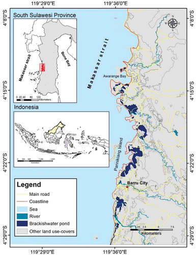
The Government of Indonesia has selected this region as one of the central development locations for aquaculture. The local government is encouraging diversification of land use. With the expectation of high economic return, a large intertidal area has been converted into fish ponds. In the last two decades, the development of brackish water aquaculture, hereafter abbreviated as BA, has led to the conversion of agricultural lands (rice field or mixed garden) close to the coastal zone; these areas were previously forested with mangroves. However, many ponds are unproductive or abandoned because they were developed in problematic areas (Tarunamulia 2008). Unfortunately, these abandoned ponds cannot be easily converted back to other land uses such as rice fields in the short term as they are now saline and topsoil has been stripped away.

2.2. Data sets and software

This study utilized readily available spatial data at the map scale of 1:50,000, consisting of digital elevation data, land cover-use maps and locally observed tide data. Digital elevation data for the study were generated from the combination of local land surveys using a Nikon® Digital Theodolite NE-102, topographic maps and bathymetric maps (BIG 1999). Land cover-use maps were acquired from the Indonesian National Agency for Geospatial Information (known in Indonesia under the acronym BIG). Fifteen days of tide measurements using a tide staff were made at Awerange Bay and Pannikiang Island.

These local tide data were then compared to the national tide prediction published by the Hydro-oceanographic office of Indonesia (Dishidros-AL 2008) at the same time and location for quality assurance purposes. Most spatial data (vector) and raster data were analysed using GIS software, i.e. ArcGIS® version 10.0 (ESRI 2010). Fuzzy logic operations were performed mainly with ArcGIS® 10.0, but pre-evaluation of suitable membership functions and grades was done in Matlab® (MathWorks 2013). These combined analytical tools were used to create a suitability map for each sub-model and the final suitability map from the resulting sub-models.

2.3. Model development and analysis

In this study, fuzzy set techniques were employed for their ability to deal with imprecise and uncertain data associated with natural variation of environmental factors or variables such as topography and soil characteristics in the landscape (Braimoh, Vlek, and Stein 2004; Burrough, McDonnell, and Lloyd 2015; Metternicht 2003). This uncertainty is due to the natural variation of an environmental variable which is a very common issue in environmental modelling, mapping, evaluation and prediction work (Burrough, McDonnell, and Lloyd 2015; Malins and Metternicht 2006). One or more environmental variables were generated as data input for a thematic map. Lu et al. (2012) defined each input of the thematic map as a ‘factor’ used to assess habitat suitability for wild herb conservation and management. This definition of ‘factor’ is used hereafter in this paper.

The fuzzy classification process involved selecting appropriate membership functions and parameters; these were used to determine membership values for the selected spatial data sets, to establish weights for the membership values and to combine weighted membership values (Burrough, McDonnell, and Lloyd 2015). This study used fuzzy membership functions to transform the input raster of chosen or key factors into a 0–1 scale, indicating the degree of membership or fuzzy set. The fuzzy set indicates the gradual membership of each environmental factor under consideration to the suitability levels for extensive BA. A full grade of membership implies a full member of the suitable class, and a grade of 0 indicates a non-member or not-suitable class for BA.

Using the aforementioned primary datasets and analytical steps, three sub-models were then generated as factors for the small-scale suitability analysis, including water availability, buffer zone and land conversion. Besides considering the availability of the coastal spatial dataset, the three sub-models were chosen for their ability to delineate suitable and unsuitable areas and to cover physical land suitability issues and constraints (i.e. potential conflicts with adjacent land uses and priority areas for mangrove conservation) in an extensive brackish water aquaculture system. The output is mainly designed for scoping potential areas (pre-selection process) for extensive brackish water aquaculture at a national or regional level. Therefore, a more detailed analysis with more complex factors such as soil and water quality, pond engineering suitability and socio-economics analysis can be undertaken within the identified potential area. Figure 2 summarizes the general steps followed to develop the three sub-models and the final suitability models.

Figure 2. Methodological flow diagram of the fuzzy set site suitability assessment approach: this flow chart shows the main methodological pathways, based on the sub-models and related available data sets, to develop the final land suitability map.

As can be seen from Figure 2, a combination of digital elevation data of coastal areas and tide data generated the water availability sub-model. The tide data were used to determine tide-important surfaces, also called tide reference datums, such as the mean high-water spring tides (MHWS), mean high-water neap tides (MHWN) and mean tide level (MTL) for the vertical referencing purpose. The tide reference datums were calculated from principal tidal constituents using the harmonic method of tidal analysis (Boon 2004; Bose et al. 1991). The principal tidal constituents comprise the main diurnal (K1 and O1) and semidiurnal (M2, N2 and S2). A tidal constituent is characterized by a fixed tidal period but with spatially varying amplitude and phase (Boon 2004; Bose et al. 1991). In this model, all elevation data were referenced to a locally defined MTL as equivalent to the local mean sea level (MSL). The maximum reach of the high tide (the boundary between intertidal and supra-tidal) was determined according to the maximum MHWS value. Thus, a suitable area is generally defined as low-lying coastal areas that are tidally inundated or potentially inundated with less excavation or pumping. Locations that do not meet these technical requirements are considered to be unsuitable.

The fuzzy set of water availability considered the variation in MHWS values and the practicability of low-cost methods to increase water availability or tidal reach. With this sub-model, the sigmoid membership function was used to define the membership values of the fuzzy set. A membership value equal to 1 in coastal areas indicates optimum access to tidal water supply, whilst membership values close or equal to 0 represent areas with less or no access. Theoretically, coastal areas with an elevation higher than 3 m above MSL are in the category of unsuitable areas (low to no availability of seawater) due to the high investment required for land preparation and pumping (Kapetsky, McGregor, and Nanne 1987). Accordingly, these areas should have a fuzzy membership grade of 0. Therefore, this study assigned gradual fuzzy membership values to areas lying between 1.5 and 3 m from MSL to represent a class of potential areas. Despite the high availability of seawater, the sub-tidal or sea region is unsuitable for most land-based aquaculture due to drainage problems, so this region has a membership value of 0. The same applies to coastal areas near big rivers that likely have water quality problems, such as low salinity, turbidity and high sedimentation rates during the wet season. Using the ArcMap calculator, a sigmoid fuzzy membership function was employed to create the fuzzy water availability set (equation 1).

(1) $\mathrm{F}\mathrm{W}\mathrm{A}=\frac{1}{1+e^{a\left(x-c\right)}}=\hspace{0.17em}1\hspace{0.17em}/\left(1\hspace{0.17em}+\mathrm{E}\mathrm{x}\mathrm{p}\left(\left(3\right)\hspace{0.17em}\ast \hspace{0.17em}\left({ }^{\prime \prime }{\mathrm{x}}^{\prime \prime }\hspace{0.17em}-\hspace{0.17em}1.5\right)\right)\right)$(1)

where:

FWA = Fuzzy set water availability

a = parameter governing the shape of the function

c = cross-over point (grade membership = 0.5)

x = elevation data

The second sub-model is the fuzzy set of land conversion. The suitability of an existing land use-cover to be converted to BA reflects the amount of time and investment required for its conversion (Giap, Yi, and Yakupitiyage 2005). In this case, a highly suitable class of land use-cover of the land describes the situation in which minimum time and money are needed to sustainably and profitably develop the aquaculture system on it. On the contrary, the ‘not-suitable’ area indicates a maximum requirement. Therefore, the same type of land use-cover can have different weights concerning its location depending on proximity to the coastline. For example, the land-use type of coconut plantation, located in the intertidal zone, is classified as a suitable location for extensive or semi-intensive BA, but not suitable if located in the supra-tidal zone. The fuzzy set for land use-cover was created by overlaying the fuzzy set of water availability and binary-weighted land use-cover using the suitability rates in Table 1. Before overlaying, the land use-cover suitability values were first divided by the maximum suitability rate = 3, transforming the suitability values into a 0–1 scale. In this land use-cover model, sea and river regions are considered restricted areas due to drainage problems and conservation issues.

Table 1. Land-use cover types and their land suitability rates for extensive and semi-intensive BA development under the small-scale approach.

Different types of land-use cover based on their degree of suitability	Remarks	Suitability rating for the conversion
Highly suitable Existing ponds Coconut plantations Grassland/coastal swamp	The land-use cover types still receive enough water during mean highest tide level (submerged during mean highest spring tide.) Time-efficient and low construction cost.	3
Moderately suitable Saltfarm Grazing land Rice field Mixed-garden	The land-use cover types of this category are located mainly above mean highest tide level so that additional cost and extra time are necessary for reconstruction to provide adequate water availability. Although this land has been assigned for specific land use, the productivity is relatively low due to the influence of saline (salt) water.	2
Marginally suitable Agriculture land: dry land or irrigated land and mixed-garden	Technically, these land usages can still be converted to extensive or semi-intensive land-based aquaculture; however, the process requires high investment (time and cost). In addition, the productivity of the current land uses is relatively high, and converting them into other land uses (brackish water ponds) might affect the productivity of adjoining land uses.	1
Not suitable Primary mangrove Settlements/residential areas) River areas (small or big) Rain forest Other land-use covers Public facility: funeral, landing base for fishing boats, etc.	These existing land uses and covers are better maintained or protected considering their extent of productivity and their conservation function.	Restricted

Source: Modified from Poernomo (1992) and Giap et al. (2005).

This table demonstrates how different factors can influence the final rating for suitability for conversion.

The buffer zone model, which is the last sub-model, was generated following the definition of the coastal buffer zone in the Regulation of the Ministry of Marine Affairs and Fisheries, Indonesia, Reg. No 21/PERMEN-KP/2018 concerning technical guidelines for determining a coastal buffer zone. According to the ministry regulation, coastal areas within 100 m, measured from the coastline landward, must be conserved for a coastal green belt. Moreover, The Ministry of Public Works and Housing of The Republic of Indonesia regulates a distance of 50 m measured perpendicular to both sides of a small river (river basin area <500 km²) to be conserved for a riparian buffer zone (Reg. No. 28/PRT/M/2015). Since the fuzzy land use model has taken the water availability model, only two models were considered in the final analysis. Because coastal and riparian areas within the buffer zone model were assigned to restricted areas, the buffer zone line must be clearly drawn to encourage the implementation of relevant regulations and facilitate monitoring. The buffer zone model was then added to the fuzzy land-use model to produce the final fuzzy land suitability map.

A binary-weighted analysis was performed to compare the fuzzy set analyses. The binary-weighted method used the same input thematic maps and criteria as in fuzzy set analysis except for the water availability model. With the binary-weighted approach, the distance to sea criterion was used to construct the water availability model, by which land located less than 1 km from the sea is categorized as highly suitable; on the contrary, land greater than 3 km from the sea is categorized as unsuitable (Giap, Yi, and Yakupitiyage 2005). The final suitability was analysed following the weighted overlay method as in equation (2) (Bonham-Carter, 1994). With the binary-weighted method, the map classes occurring on each input map (thematic map) were assigned different scores, and the maps also received weight scores. The weights or scores (on a scale of 1–3) were given based on the level of importance of a particular factor that influences BA, where 3 represents the greatest meaning, and 1 has the least meaning. Constraints such as conservation area or waterbody (sea or river) were scored as 0 to exclude them from suitability analysis. The weighted overlay analysis was performed in the ArcGIS model builder.

(2) $\mathrm{S}\mathrm{u}\mathrm{i}\mathrm{t}\mathrm{a}\mathrm{b}\mathrm{i}\mathrm{l}\mathrm{i}\mathrm{t}\mathrm{y}=\frac{{\sum }_i^n{S}_{ij}{W}_i}{{\sum }_i^{n}Wi}$(2)

where W_i is the weight for the ith input map, and S_ij is the score for the jth class of the ith input map. The final suitability classes are presented as highly suitable, moderately suitable, marginally suitable and not suitable.

3. Results

3.1. Water availability model

It is estimated that land with elevation ≥25 m accounts for about 78% of the total landscape in Barru District (BIG 1999). Furthermore, a detailed field survey indicates that 17,467 ha occurs within a distance of 3.5 km landward from the coastline, and about 3,800 ha or 21% of the coastal area has a ground elevation equal to or less than 3 m. More than 80% of these low-lying tidal flats are currently used for extensive BA. This is due to the proximity to the sea which allows tidal energy and a short length of canals to provide a low-cost water supply for the aquaculture system.

As summarized in Table 2, there is clear variability in tide amplitudes for major tidal constituents from one place to another within the study area. This variation in amplitudes does not influence tide type over the study area which is classed as mixed type with diurnal dominance (Formzhal; ‘F’ = 1.62 to 2.24) (Boon 2004; Bose et al. 1991). However, variation in amplitude values of the major tidal constituents results in different MHWS values ranging from 0.90 to 1.21 m (1.05 ± 0.15 m). These varied MHWS values indicate that coastal areas with optimal accessibility to tidewater supply are between 0 and 1.5 m above local MSL.

Table 2. Comparison of primary tidal constituents and their resulting amplitudes for three different locations within the study site. The primary tidal constituents are key for the water availability model given that extensive systems largely rely on tides to provide and remove water from the ponds.

Tidal constituent	Amplitude (m)
	Pannikiang island	Awerange bay	Biringkassi island^a
M2 (main lunar semidiurnal)	0.19	0.09	0.13
S2 (main solar semidiurnal)	0.07	0.17	0.17
N2 (larger lunar elliptic semidiurnal)	0.06	0.04	0.05
K1 (lunar–solar declination diurnal)	0.43	0.29	0.32
O1 (lunar declination diurnal)	0.17	0.15	0.20
MHWS	1.21	0.9	1.04

*= (Dishidros-AL 2008).

The primary tidal constituents are key for the water availability model given that extensive systems largely rely on tides to provide and remove water from the ponds.

^aDishidros (2008).

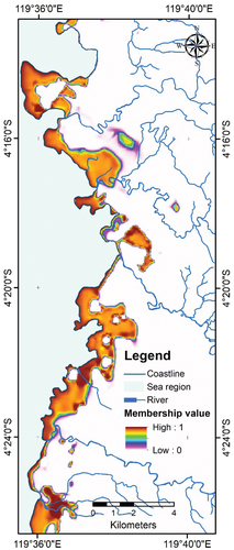
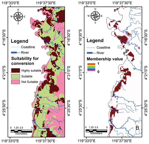
Figure 3 shows the fuzzy membership of coastal areas in terms of water availability for extensive BA. The total area representing the maximum grade of fuzzy memberships (0.8– to 1.0) covers about 15% (2745.7 ha) of the total 17,467.8 ha of the coastal area. This sub-model estimates that the tide could reach a maximum distance of 2.5 km landward, relying only on natural variations of land slope or elevation within the region. This model also suggests that some areas represented by a membership value near zero (in purple colour) are potentially expanded further landward, particularly in areas adjacent to existing rivers or tidal creeks.

Figure 3. Fuzzy set representation of water availability. The fuzzy set shows the dominance of high membership values along the coastal fringe where BA is concentrated.

3.2. Land conversion model

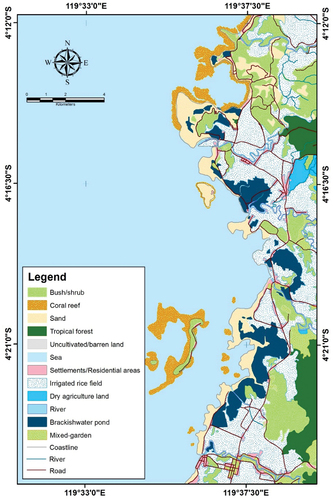
At the scale of 1:50,000 for land-use cover base maps, the land use can only be divided into 10 major classes (Figure 4). Forestry (both protected and limited-production tropical forest) is a major land use in Barru covering about 47% of the total available land. This is followed by mixed-gardens and rice fields which account for 15% and 11% of land use, respectively. The dominant land-uses or covers within 3.5 km from the coastline are irrigated rice fields, shrub-land, brackish water fish/shrimp ponds, sand dunes and settlements which account for 40%, 28%, 9%, 8%, 6% and 4% of the total area 17,467 ha, respectively.

Figure 4. Land-use/-cover map of Barru District. The map shows that extensive areas of rice still remain despite the rapid conversion of this land use to BA within the region. Unsurprisingly, and undeveloped sandy zone remains.

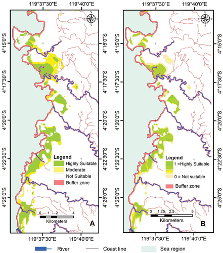
Maps in Figure 5 show the suitability ratings of existing land-use cover to be converted to BA. Using the land-use cover suitability rate from the aforementioned Table 1, the suitability classes for extensive brackish water aquaculture systems in this study area can be classified as highly suitable, moderately suitable and not suitable (Figure 5A). A highly suitable class of land-use cover comprises existing brackish water ponds, irrigated rice fields, shrubland, dry agricultural land and mixed-gardening, which are located in the intertidal zone. Not-suitable areas include sand dunes, settlements, rain-fed rice fields and tropical rainforests. The fuzzy land conversion model provides rank differences of the land-use cover types and the degree to which land-use cover located near existing brackish water ponds could be converted to brackish water ponds (Figure 5B).

Figure 5. Suitability for land conversion model comparing the binary-weighted land conversion model (A) to the fuzzy land conversion model (B).

3.3. Buffer zone model

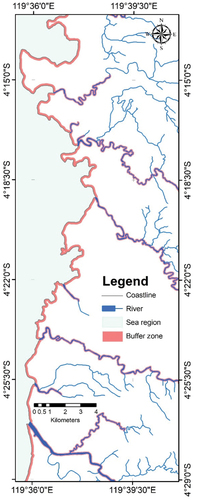
The buffer zone model for a combined coastal green belt and riparian buffer zone is illustrated in Figure 6. This buffer zone is a typical protected areas that are very likely influenced by the rapid development of extensive BA. This buffer zone consists primarily of mangrove and riparian areas. This buffer zone not only limits BA activities but also other land uses. If the buffer zone model is overlain with the land use-cover map, it is clear that some of the buffer zone areas have been utilized as settlements, brackish water ponds and irrigated rice fields.

Figure 6. Green-belt buffer zone model combining coastal and riparian buffer zone: because of a lack of site selection and compliance with development policies and laws, some of the buffer zone is already impacted by BA.

3.4. Final land suitability

Figure 7 presents the final suitability maps comparing the result of the binary-weighted overlay and fuzzy membership values partitioning method. Land suitability classes in the binary approach suitability map comprise not suitable, moderately suitable and highly suitable (Figure 7A). With the fuzzy set approach, the membership value indicates the degree of suitability for BA at a given location concerning given land characteristics (Figure 7B). The first interesting thing to note from those figures is that the total area identified for highly and moderately suitable classes is lower with the fuzzy set approach than with the binary-weighted approach. The significant difference can be seen from the total area for the moderately suitable area, which covers 914 ha for the binary approach and only 311 ha for the fuzzy set approach. The difference of 600 ha is currently used for irrigated rice fields having elevation more than 3 m above mean sea level. If the coastal area is clipped within 3.5 km from the coastline, the estimated total area assigned to the not-suitable class is 13,032 ha for the binary approach, which is lower than the lowest fuzzy membership values of the fuzzy set approach (13676 ha). The difference in estimation results, especially in the moderately suitable class, was mainly due to how the water availability criteria are defined. The fuzzy set approach considers land elevation and local tides, while the binary-weighted approach only uses the relative distance from seawater sources or coastlines.

Figure 7. Final land suitability map: (A) weighted overlay output; (B) fuzzy set representation. Clearly, there are differences in the land identified as suitable between the two approaches, with the fuzzy set representation showing less area as highly or moderately suitable.

4. Discussion

Water availability provides a straightforward estimation of the areas potentially suitable for extensive BA. This sub-model estimated that the available coastal area for BA is no more than 3% of the regency’s total area. This alarmingly small area is already under pressure from BA development. The efficacy of using water availability as a factor in this study corroborates the study conducted by McLeod et al. (2002), who found that the distance to water or water availability constraint is the most effective method to identify unsuitable areas for land-based coastal aquaculture. An extensive brackish water aquaculture system depends on low technology and minor inputs, and the water supply is influenced primarily by the local tidal range and land elevation (Anyawu et al. 2007; Chowdhury et al. 2000; Howerton 2001; Lekang 2007). This is the main reason why most existing ponds are concentrated primarily in the middle and southern parts of the district, where the coastal relief is gentle. With an average tidal range of less than 1.5 m, the available intertidal area seems more suitable for milkfish than shrimp culture (Requintina, Mmochi, and Msuya 2008). The integration of fuzzy set in the sub-model of water availability helped to improve the approximation of the uncertainty regarding the local variation of tidal ranges and possible technology inputs such as employing limited pumping and extending canal networks. Thus, the graded membership values indicated a naturally available water source and possible local ways of increasing the availability. At locations with gradation values, obtaining additional spatial information, such as the status of existing land uses, is still necessary to enrich the information for effective spatial decision-making.

The second sub-model of land conversion provides types of existing land-use cover at the landward boundary that have been or could be potentially converted to brackish water ponds. Unlike the old approach of using a binary classification scheme for the land-use types, which provides limited information on different land-use cover categories or ranks (Ghobadi, Nasri, and Ahmadipari 2021; Hossain and Das 2012); this developed fuzzy-based approach enables further differentiation of qualities of the same category. For example, it is possible to differentiate brackish water ponds located in different tidal zones (intertidal and supra-tidal) or shrubs located either in mangroves areas in the intertidal zone or live in association with rain forest in the supra-tidal zone. Because the gradual degree of memberships of land-use cover at boundary areas combines the weights of land-use cover and the fuzzy membership of water availability, it can also indicate possible saltwater intrusion in the existing land-use cover. Past studies reported that the failure of vegetable and rice crops had been attributed to shrimp farming due to seawater intrusion and salt contamination of the coastal groundwater systems (Azad, Jensen, and Lin 2009; Teng 2008). In addition, Pattanaik and Narendra Prasad (2011) and Debnath (2021) identified social conflicts, consisting of disputes over land use rights, unequal wealth distribution and reduced quality of freshwater as significant impacts from aquaculture development on existing land uses.

Using the fuzzy set technique in the land conversion sub-model adds predictive capacity to the resulting map. This is more noticeable at locations with overlapping boundaries of two or more land uses, as indicated by partial membership values. The predictive ability includes the prediction of the magnitude and direction of the land conversion, for instance, from rice fields to shrimp ponds and vice versa, or other land-use types. Thus, it is very helpful as preliminary information to help predict potential conflicts over land use rights or allocations. For aquaculture decision-makers in particular, this type of spatial representation can be useful information for selecting the most suitable aquaculture system, such as extensive, semi-intensive or intensive. As an example, land located in the supra-tidal zone is, by definition, unsuitable for extensive aquaculture due to natural tidewater exchange limitations, but it could be suitable for intensive aquaculture if the cost of pumping is still feasible. This sub-model can also be used to identify the degree of surrounding ecosystems that could be impacted by the magnitude and direction expansion of BA.

Even without the government rule for green-belt protection, the pond development must not be allowed to expand to mangrove areas for suitability reasons. Many studies have also shown that mangroves are not a good site for BA due to high percentage of organic matter, a high level of soil acidity and drainage difficulties of low-lying land, and disease risks (Ahmad, Tjaronge, and Suryati 2003; Boyd, Davis, and McNevin 2022; Islam and Wahab 2005; Primavera 1998; Sonnenholzner and Boyd 2007). Several studies reported that shrimp or fish farmers seem unaware or recalcitrant because they keep extending their farming area within the mangrove buffer zone (Ashton 2008; De Lacerda et al. 2021; Elwin et al. 2019). This is likely due to the absence of adequate spatial information on the conservation zone to regulate the conversion activity and a lack of enforcement of legal instruments meant to manage development. The last ‘green belt’ or buffer zone sub-model could be a useful model to support the implementation of national, regional and international policies and strategies for protecting mangrove environments. Attempts at protecting mangrove ecosystems for the sustainability of aquaculture have also been particularly encouraged in Part I of the code of practice for responsible shrimp farming published by Global Aquaculture Alliance (Boyd 1999), in that BA should not be developed within mangrove ecosystems. Environmental managers could utilize this map to monitor proposed or ongoing activities, including aquaculture in the buffer zone. This spatial information on conservation can be used to immediately implement appropriate legislation to effectively manage aquaculture activities located near the mangrove buffer zone areas, for both extensive and intensive systems. This is in line with the concept of ecologically friendly aquaculture practices as discussed in the FAO Code of Conduct for Responsible Fisheries (Nordquist, Nandan, and Kraska 2012) and the concept of ‘ecological well-being’ in the second objective of the FAO’s EAA (Aguilar-Manjarrez, Kapetsky, and Soto 2010).

The final land suitability maps further confirm the difference and thus the clear advantage of using the fuzzy set approach instead of a binary weighted approach. The major difference can be seen from the exact assessment method of suitability level demonstrated with binary logic. This binary approach has the advantage for quick and easy interpretation, but at the same time, it can also be a risky process because of the potential to over or underestimate. Whereas the fuzzy set approach provides continuum location values of membership to the suitability class, and, therefore provides an advantage for identifying variations even within the same suitability class. This enables a flexible opportunity for the decision-making process for aquaculture development. Fuzzy membership of locations to land suitability categories allows us to identify the presence of one or more key limiting supporting variables at a specific location. Given this, the limiting factor should be carefully considered if the effort is made to develop a potential area. In practice, understanding the presence and nature of the limiting factors is meaningful, particularly in the category of ‘potentially’ or ‘less suitable’ because it will assist decision-makers or aquaculture stakeholders in making decisions about proper land management. For example, farmers could employ technologies to manage the limiting factors to help shift the status of being a ‘potentially suitable’ class to being a ‘suitable class’. Additionally, limiting factors in the class of potential areas might be in reality so difficult to manage that the planning decision is to recommend a land use other than aquaculture. The land conversion model in the particular locations might not be suitable for extensive brackish water systems but potentially suitable for other aquaculture systems such as those classified as semi-intensive or intensive.

As described in the sub-model of land conversion, the fuzzy set approach is useful due to its predictive ability to identify potential areas for development. This capability is crucial to anticipate potential conflicts with other land uses, especially for BA development. Looking at the result of the fuzzy set for moderately suitable class in the supra-tidal area, area expansion is possible, especially where there are rivers or extended canals. In this case, the productivity status of existing land uses such as agriculture, e.g. mixed-garden rice fields, adjacent to existing BA ponds determines the decision-making process for conversion. However, it is also important to note that the total area for the suitable class assigned to coastal areas near the coastline (often mangrove areas) seems to be overestimated with the fuzzy set approach. This could be due to the relatively high grade of membership values assigned to this location’s fuzzy set of water and land-use cover sub-models. The same phenomenon was also experienced by Malins and Metternicht (2006) who found the underperformance of fuzzy landscape analysis GIS (FLAG) for salinity mapping which they believe is due to the choice of either the fuzzy membership function or the fuzzy operator used to integrate map layers.

Like other products of land suitability mapping at the same geographical scale, these suitability levels are only relevant to the ‘pre-selection process’ and for dealing with complex spatial datasets to support aquaculture planning purposes at a national or regional level (McLeod, Pantus, and Preston 2002). Within a ‘suitable area’ defined in this map, the suitability likely varies with the increase in map ratio or a larger-scale map, and as more environmental variables such as soil and water quality are included in the analysis. Therefore, the suitability levels as presented in the final map of suitability, are not an exact assessment or final suitability information; hence, it is not necessarily presented in a sharply defined class boundary but by a natural continuum membership.

5. Conclusion and recommendation

Overall, the fuzzy-based GIS approach proposed in this study provides adequate information for national aquaculture planning purposes. Although employing limited key environmental variables, it effectively covers physical land suitability issues and constraints in extensive brackish water aquaculture systems, which is one of the central goals of small-scale site assessment. It provides technical flexibility for the GIS analyst to handle a poor data environment without diminishing the quality of the map outputs. In terms of the methodological perspective, integrating fuzzy set techniques in this approach improves the assessment, presentation and information quality of the natural characteristics of the environmental data. Classification outputs presented on a continuous scale by a means membership function are more informative than the hard partition approach. This is most noticeably important in the boundary areas between two different classes for each environmental variable under study. The fuzzy set techniques, however, might be criticized for not providing definite suitability classes. However, for national or provincial aquaculture decisional makers, this could be the best-generalized approach for obscure information that is sensitive to a correct decision.

This approach is expected to be a quick site assessment tool, compensating for the absence of a quick spatial assessment method and an alternative that overcomes the complexity of the multi-criteria assessment method. It should also be noted that this proposed practical and conceptual spatial analyses framework is not limited to the proposed key environmental variables only; there is potential to apply it to other environmental variables such as soil characteristics at the same cartographic or map scale whenever the data are available. Moreover, the output broad-scale suitability map should not be forced to over-explain technical aspects or farm level of BA aquaculture management. Therefore, a finer scale approach is necessary to improve detail as well as accuracy.

Acknowledgements

The authors wish to thank the Australian Centre for International Agricultural Research (ACIAR) for funding projects associated with this paper. We also thank the Research Institute for Coastal Aquaculture and Fisheries Extension (RICAFE), Indonesia and School of Biological, Earth and Environmental Sciences, The University of New South Wales (UNSW) for access to various resources and facilities during spatial data collection and analysis.

Disclosure statement

The authors declare that they have no known competing financial interests or personal relationships that could have appeared to influence the work reported in this paper.

References

- Aguilar-Manjarrez, J., J. Kapetsky, and D. Soto, 2010. “The Potential of Spatial Planning Tools to Support the Ecosystem Approach to Aquaculture.” FAO Fisheries and Aquaculture Technical Paper. 176.
- Ahmad, T., M. Tjaronge, and E. Suryati. 2003. “Performances of Tiger Shrimp Culture in Environmentally Friendly Ponds.” Indonesian Journal of Agricultural Science 4 (2): 48–55. https://doi.org/10.21082/ijas.v4n2.2003.p48-55.
- Anand, A., P. Krishnan, A. S. Suryavanshi, S. B. Choudhury, G. Kantharajan, C. Srinivasa Rao, C. Manjulatha, and D. E. Babu. 2021. “Identification of Suitable Aquaculture Sites Using Large-Scale Land Use and Land Cover Maps Factoring the Prevailing Regulatory Frameworks: A Case Study from India.” Journal of the Indian Society of Remote Sensing 49 (4): 725–745. https://doi.org/10.1007/s12524-020-01211-7.
- Anyawu, P. E., U. U. Gabriel, O. A. Akinrotimi, D. O. Bekibele, and D. N. Onunkwo. 2007. “Brackish Water Aquaculture: A Veritable Tool for the Empowerment of Niger Delta Communities.” Scientific Research and Essays 2:295–301.
- Ashton, E. C. 2008. “The Impact of Shrimp Farming on Mangrove Ecosystems.” CAB Reviews: Perspectives in Agriculture, Veterinary Science, Nutrition & Natural Resources 3 (January 2010). https://doi.org/10.1079/PAVSNNR20083003.
- Ateweberhan, M., J. Hudson, A. Rougier, N. S. Jiddawi, F. Msuya, S. M. Stead, and A. Harris. 2018. “Community Based Aquaculture in the Western Indian Ocean: Challenges and Opportunities for Developing Sustainable Coastal Livelihoods.” Ecology and Society 23 (4): 17. https://doi.org/10.5751/ES-10411-230417.
- Azad, A. K., K. R. Jensen, and C. K. Lin. 2009. “Coastal Aquaculture Development in Bangladesh: Unsustainable and Sustainable Experiences.” Environmental Management 44 (4): 800–809. https://doi.org/10.1007/s00267-009-9356-y.
- Bagarinao, T., and J. Primavera 2005. “Code of Practice for Sustainable Use of Mangrove Ecosystems for Aquaculture in Southeast Asia.” Ecosystems. https://core.ac.uk/download/pdf/10863435.pdf.
- Bandira, P. N. A., M. A. Mahamud, N. Samat, M. L. Tan, and N. W. Chan. 2021. “Gis-Based Multi-Criteria Evaluation for Potential Inland Aquaculture Site Selection in the George Town Conurbation, Malaysia.” Land 10 (11). https://doi.org/10.3390/land10111174.
- BIG. 1999. Topographic Maps of Barru District, Scale of 1 to 50,000. Cibinong-Bogor, Indonesia: National Coordination for Survey and Mapping.
- BMKG. 2018. “Weather and Climate of Barru District [WWW Document].” Meteorological Climatol Geophysics Agency. Accessed January 12, 2018. https://www.bmkg.go.id/?lang=EN.
- Bonham-Carter, G. F. 1994.“Geographic Information Systems for Geoscientists.“ In Computers & Geosciences, edited by D. F. Merriam, 1st ed., Vol. 1. Elsevier. https://doi.org/10.1016/C2013-0-03864-9.
- Boon, J. D. 2004. Secrets of the Tide: Tide and Tidal Current Analysis and Predictions, Storm Surges and Sea Level Trends, Secrets of the Tide: Tide and Tidal Current Analysis and Predictions, Storm Surges and Sea Level Trends. Chichester, U.K: Horwood Publishing. https://doi.org/10.1016/C2013-0-18114-7.
- Bórquez-Lopez, R. A., R. Casillas-Hernandez, J. A. Lopez-Elias, R. H. Barraza-Guardado, and L. R. Martinez-Cordova. 2018. “Improving Feeding Strategies for Shrimp Farming Using Fuzzy Logic, Based on Water Quality Parameters.” Aquacultural Engineering 81 (August 2017): 38–45. https://doi.org/10.1016/j.aquaeng.2018.01.002.
- Bose, A. N., S. N. Ghosh, C. T. Yang, and A. Mitra. 1991. Coastal Aquaculture Engineering, Choice Reviews Online. New York: Edward Arnold. https://doi.org/10.5860/choice.29-3915.
- Boyd, C. E. 1999. Codes of Practice for Responsible Shrimp Farming. Global Aquaculture Alliance. https://www.amazon.com/Codes-practice-responsible-shrimp-farming/dp/096700960X.
- Boyd, C. E., R. P. Davis, and A. A. McNevin. 2022. “Perspectives on the Mangrove Conundrum, Land Use, and Benefits of Yield Intensification in Farmed Shrimp Production: A Review.” Journal of the World Aquaculture Society 53 (1): 8–46. https://doi.org/10.1111/jwas.12841.
- Braimoh, A. K., P. L. G. Vlek, and A. Stein. 2004. “Land Evaluation for Maize Based on Fuzzy Set and Interpolation.” Environmental Management 33 (2): 226–238. https://doi.org/10.1007/s00267-003-0171-6.
- Burrough, P. A., R. A. McDonnell, and C. D. Lloyd. 2015. Principles of Geographical Information Systems. 3rd ed. Oxford, United Kingdom: Oxford University Press.
- Carbajal-Hernández, J. J., L. P. Sánchez-Fernández, J. A. Carrasco-Ochoa, and J. F. Martínez-Trinidad. 2012. “Immediate Water Quality Assessment in Shrimp Culture Using Fuzzy Inference Systems.” Expert Systems with Applications 39 (12): 10571–10582. https://doi.org/10.1016/j.eswa.2012.02.141.
- Chowdhury, M. A. K., R. B. Shivappa, J. Hambrey, A. Resources, and M. Program 2000. “Concept of Environmental Capacity, and Its Application to Planning and Management of Coastal Aquaculture.” Aquaculture, August 2014. https://doi.org/10.13140/2.1.4178.8801.
- CSAR. 2006. Soil Map and Agro-Ecology. Bogor, Indonesia: Central for Soil and Agroclimate Research.
- Debnath, R. 2021. “Conflicts Over Water and Land Use in Coastal Aquaculture Vis-à-Vis Fisheries Conflicts Over Water and Land Use in Coastal Aquaculture Vis-à-Vis Fisheries.” NESFA Journal of Fisheries and Aquaculture 1 (1): 12–14.
- De Lacerda, L. D., R. D. Ward, M. D. P. Godoy, A. J. D. A. Meireles, R. Borges, and A. C. Ferreira. 2021. “20-Years Cumulative Impact from Shrimp Farming on Mangroves of Northeast Brazil.” Frontiers in Forests and Global Change 4 (April). https://doi.org/10.3389/ffgc.2021.653096.
- Diep, N. T. H., T. Korsem, N. T. Can, W. Phonphan, and V. Q. Minh. 2019. “Determination of Aquaculture Distribution by Using Remote Sensing Technology in Thanh Phu District, Ben Tre Province, Vietnam.” Vietnam Journal of Science, Technology and Engineering 61 (2): 35–41. https://doi.org/10.31276/vjste.61(2).35-41.
- Dishidros-AL. 2008. Tide Tables: Indonesian Archipelago. Jakarta Utara, Indonesia: Indonesia Hydro-Oceanographic Office.
- Elwin, A., J. J. Bukoski, V. Jintana, E. J. Z. Robinson, and J. M. Clark. 2019. “Preservation and Recovery of Mangrove Ecosystem Carbon Stocks in Abandoned Shrimp Ponds.” Scientific Reports 9 (1): 1–10. https://doi.org/10.1038/s41598-019-54893-6.
- ESRI. 2010. “ArcGis 10.0, from Environmental Systems Research Institute (ESRI) [WWW Document].” http://www.esri.com.
- Falconer, L., A. L. Middelboe, H. Kaas, L. G. Ross, and T. C. Telfer. 2020. “Use of Geographic Information Systems for Aquaculture and Recommendations for Development of Spatial Tools.” Reviews in Aquaculture 12 (2): 664–677. https://doi.org/10.1111/raq.12345.
- Falconer, L., T. Telfer, K. L. Pham, and L. Ross 2017. “GIS Technologies for Sustainable Aquaculture.” In Comprehensive Geographic Information Systems, (Vol. 3). Elsevier. https://doi.org/10.1016/B978-0-12-409548-9.10459-2.
- Ghobadi, M., M. Nasri, and M. Ahmadipari. 2021. “Land Suitability Assessment (LSA) for Aquaculture Site Selection via an Integrated GIS-DANP Multi-Criteria Method; a Case Study of Lorestan Province, Iran.” Aquaculture 530 (July 2020): 735776. https://doi.org/10.1016/j.aquaculture.2020.735776.
- Giap, D. H., Y. Yi, and A. Yakupitiyage. 2005. “GIS for Land Evaluation for Shrimp Farming in Haiphong of Vietnam.” Ocean & Coastal Management 48 (1): 51–63. https://doi.org/10.1016/j.ocecoaman.2004.11.003.
- Gimpel, A., V. Stelzenmüller, S. Töpsch, I. Galparsoro, M. Gubbins, D. Miller, A. Murillas, et al. 2018. “A GIS-Based Tool for an Integrated Assessment of Spatial Planning Trade-Offs with Aquaculture.” Science of the Total Environment 627:1644–1655. https://doi.org/10.1016/j.scitotenv.2018.01.133.
- González-Rivas, D. A., and F. O. Tapia-Silva. 2023. “Estimating the Shrimp Farm’s Production and Their Future Growth Prediction by Remote Sensing: Case Study Gulf of California.” Frontiers in Marine Science 10 (February): 1–8. https://doi.org/10.3389/fmars.2023.1130125.
- Hanafi, A., and T. Ahmad. 1996. “Shrimp Culture in Indonesia. Key Sustainability and Research Issues.” Paper Present ACIAR WorkEducation Hat Yai 69–74.
- Hossain, M. S., and N. G. Das. 2012. “Ecosystem Modeling in GIS-Based Multi-Criteria Evaluation for Aquaculture Development at Noakhali Coast, Bangladesh.” International Geoinformatics Research and Development Journal Ecosystem 3 (4): 1–23.
- Howerton, R. 2001. “Best Management Practices for Hawaiian Aquaculture.” In Center for tropical and subtropical aquaculture, Waimanalo, Hawaii, USA (Vol. 148) Center for Tropical and Subtropical Aquaculture.
- Huang, B., K. Cao, and E. A. Silva 2017. “Comprehensive Geographic Information Systems.” In Comprehensive Geographic Information Systems (Vol. 3, Issue August).
- Islam, M. S., and M. A. Wahab. 2005. “A Review on the Present Status and Management of Mangrove Wetland Habitat Resources in Bangladesh with Emphasis on Mangrove Fisheries and Aquaculture.” Hydrobiologia 542 (1): 165–190. https://doi.org/10.1007/s10750-004-0756-y.
- Jayanthi, M., M. Duraisamy, S. Thirumurthy, M. Samynathan, S. Kabiraj, K. Manimaran, and M. Muralidhar. 2020. “Ecosystem Characteristics and Environmental Regulations Based Geospatial Planning for Sustainable Aquaculture Development.” Land Degradation and Development 31 (16): 2430–2445. https://doi.org/10.1002/ldr.3615.
- Jayanthi, M., P. Nila Rekha, N. Kavitha, and P. Ravichandran. 2006. “Assessment of Impact of Aquaculture on Kolleru Lake (India) Using Remote Sensing and Geographical Information System.” Aquaculture Research 37 (16): 1617–1626. https://doi.org/10.1111/j.1365-2109.2006.01602.x.
- Jayanthi, M., S. Thirumurthy, M. Muralidhar, and P. Ravichandran. 2018. “Impact of Shrimp Aquaculture Development on Important Ecosystems in India.” Global Environmental Change 52 (March): 10–21. https://doi.org/10.1016/j.gloenvcha.2018.05.005.
- Kapetsky, J. M., L. McGregor, and E. H. Nanne. 1987. “A Geographical Information System and Satellite Remote Sensing to Plan for Aquaculture Development: A FAO - UNEP/GRID Cooperative Study in Costa Rica.” FAO Fisheries Technology Paper.
- Karstens, S., and M. C. Lukas. 2014. “Contested Aquaculture Development in the Protected Mangrove Forests of the Kapuas Estuary, West Kalimantan.” Geoöko 35 (January 2014): 78–121.
- Karthik, M., J. Suri, N. Saharan, and R. S. Biradar. 2005. “Brackish Water Aquaculture Site Selection in Palghar Taluk, Thane District of Maharashtra, India, Using the Techniques of Remote Sensing and Geographical Information System.” Aquacultural Engineering 32 (2): 285–302. https://doi.org/10.1016/j.aquaeng.2004.05.009.
- Kusumastanto, T., C. M. Jolly, and C. Bailey. 1998. “A Multiperiod Programming Evaluation of Brackishwater Shrimp Aquaculture Development in Indonesia 1989/1990–1998/1999.” Aquaculture 159 (3–4): 317–331. https://doi.org/10.1016/S0044-8486(97)00191-9.
- Lekang, O. I. 2007. “Aquaculture Engineering.” In Aquaculture Engineering. https://doi.org/10.1002/9780470995945
- Longdill, P. C., T. R. Healy, and K. P. Black. 2008. “An Integrated GIS Approach for Sustainable Aquaculture Management Area Site Selection.” Ocean and Coastal Management 51 (8–9): 612–624. https://doi.org/10.1016/j.ocecoaman.2008.06.010.
- Lu, C. Y., W. Gu, A. H. Dai, and H. Y. Wei. 2012. “Assessing Habitat Suitability Based on Geographic Information System (GIS) and Fuzzy: A Case Study of Schisandra sphenanthera Rehd. Et Wils. in Qinling Mountains, China.” Ecological Modelling 242:105–115. https://doi.org/10.1016/j.ecolmodel.2012.06.002.
- Macusi, E. D., D. E. P. Estor, E. Q. Borazon, M. B. Clapano, and M. D. Santos. 2022. “Environmental and Socioeconomic Impacts of Shrimp Farming in the Philippines: A Critical Analysis Using PRISMA.” Sustainability (Switzerland) 14 (5): 1–19. https://doi.org/10.3390/su14052977.
- Malins, D., and G. Metternicht. 2006. “Assessing the Spatial Extent of Dryland Salinity Through Fuzzy Modeling.” Ecological Modelling 193 (3–4): 387–411. https://doi.org/10.1016/j.ecolmodel.2005.08.044.
- MathWorks. 2013. MATLAB and Simulink Product Families. MathWorks, Inc. https://www.mathworks.com/products/new_products/release2019a.html.
- McLeod, I., F. Pantus, and N. Preston. 2002. “The Use of a Geographical Information System for Land-Based Aquaculture Planning.” Aquaculture Research 33 (4): 241–250. https://doi.org/10.1046/j.1355-557x.2001.00667.x.
- Metternicht, G. I. 2003. “Categorical Fuzziness: A Comparison Between Crisp and Fuzzy Class Boundary Modelling for Mapping Salt-Affected Soils Using Landsat TM Data and a Classification Based on Anion Ratios.” Ecological Modelling 168 (3): 371–389. https://doi.org/10.1016/S0304-3800(03)00147-9.
- MMAF. 2019. Annual Report Ministry of Marine Affairs and Fisheries, Indonesia - 2018. Jakarta.
- Nagamani, K., and Y. Suresh. 2019. “Evaluation of Coastal Aquaculture Ponds Using Remote Sensing and GIS.” Indian Journal of Geo-Marine Sciences 48 (8): 1205–1209. https://doi.org/10.13140/RG.2.2.27400.98565.
- Nayak, A. K., P. Kumar, D. Pant, and R. K. Mohanty. 2018. “Land Suitability Modelling for Enhancing Fishery Resource Development in Central Himalayas (India) Using GIS and Multi-Criteria Evaluation Approach.” Aquacultural Engineering 83:120–129. https://doi.org/10.1016/j.aquaeng.2018.10.003.
- Nguyen, H. T., T. T. Hoang, L. V. Van, I. Prakash, and T. T. Tran. 2022. “An Integrated Approach of GIS-AHP-MCE Methods for the Selection of Suitable Sites for the Shrimp Farming and Mangrove Development - a Case Study of the Coastal Area of Vietnam.” Sains Tanah 19 (1): 99–110. https://doi.org/10.20961/stjssa.v19i1.58211.
- Nordquist, M. H., S. N. Nandan, and J. Kraska. 2012. Code of Conduct for Responsible Fisheries, UNCLOS 1982 Commentary. Rome: Food and Agriculture Organization of the United Nations. https://doi.org/10.1163/9789004215627.
- Panchatcharam, K., and M. Anand. 2017. “Impact of Aquaculture Industries on Geomorphology Around Buckingham Canal, Kancheepuram District, Tamil Nadu, India Using Remote Sensing and GIS Techniques.” International Journal of Scientific Research in Science & Technology 3 (8): 142–147.
- Pattanaik, C., and S. Narendra Prasad. 2011. “Assessment of Aquaculture Impact on Mangroves of Mahanadi Delta (Orissa), East Coast of India Using Remote Sensing and GIS.” Ocean & Coastal Management 54 (11): 789–795. https://doi.org/10.1016/j.ocecoaman.2011.07.013.
- Pérez, O. M., L. G. Ross, T. C. Telfer, and L. M. Del Campo Barquin. 2003. “Water Quality Requirements for Marine Fish Cage Site Selection in Tenerife (Canary Islands): Predictive Modelling and Analysis Using GIS.” Aquaculture 224 (1–4): 51–68. https://doi.org/10.1016/S0044-8486(02)00274-0.
- Poernomo, A. 1992. Key Environmental Factors in Intensive Shrimp Ponds. A. Bittner edited by. Jakarta, Indonesia: Yayasan Obor Indonesia.
- Primavera, J. H. 1998. “Tropical Shrimp Farming and Its Sustainability.” In Tropical Mariculture, edited by S. D. Silva, 257–289. London: Academic Press. https://doi.org/10.1016/b978-012210845-7/50008-8.
- Radiarta, I. N., S. I. Saitoh, and A. Miyazono. 2008. “GIS-Based Multi-Criteria Evaluation Models for Identifying Suitable Sites for Japanese Scallop (Mizuhopecten Yessoensis) Aquaculture in Funka Bay, Southwestern Hokkaido, Japan.” Aquaculture 284 (1–4): 127–135. https://doi.org/10.1016/j.aquaculture.2008.07.048.
- Rajitha, K., C. K. Mukherjee, and R. Vinu Chandran. 2007. “Applications of Remote Sensing and GIS for Sustainable Management of Shrimp Culture in India.” Aquacultural Engineering 36 (1): 1–17. https://doi.org/10.1016/j.aquaeng.2006.05.003.
- Requintina, E. D., A. J. Mmochi, and F. E. Msuya 2008. “A Guide to Milkfish Culture in the Western Indian Ocean Region.” http://www.crc.uri.edu.
- Rubel, H., W. Woods, D. Pérez, A. Meyer, Z. Felde, S. Zielcke, C. Lidy, and C. Lanfer 2019. A Strategic Approach to Sustainable Shrimp Production in Indonesia the Case for Improved Economics and Sustainability. 53.
- Salam, M. A., N. A. Khatun, and M. M. Ali. 2005. “Carp Farming Potential in Barhatta Upazilla, Bangladesh: A GIS Methodological Perspective.” Aquaculture 245 (1–4): 75–87. https://doi.org/10.1016/j.aquaculture.2004.10.030.
- Silva, C., J. G. Ferreira, S. B. Bricker, T. A. DelValls, M. L. Martín-Díaz, and E. Yáñez. 2011. “Site Selection for Shellfish Aquaculture by Means of GIS and Farm-Scale Models, with an Emphasis on Data-Poor Environments.” Aquaculture 318 (3–4): 444–457. https://doi.org/10.1016/j.aquaculture.2011.05.033.
- Sonnenholzner, S., and C. E. Boyd. 2007. “Vertical Gradients of Organic Matter Concentration and Respiration Rate in Pond Bottom Soils.” Journal of the World Aquaculture Society 31 (3): 376–380. https://doi.org/10.1111/j.1749-7345.2000.tb00887.x.
- Tarunamulia, 2008. Application of Fuzzy Logic, GIS, and Remote Sensing to the Assessment of Environmental Factors for Extensive Brackishwater Aquaculture in Indonesia. MSc-Thesis Sch. Biological Earth Environmental Science Faculty Science. University of New South Wales (UNSW).
- Tarunamulia, and J. Sammut. 2022. “An Evaluation of the Engineering Suitability of Extensive Brackishwater Ponds in Barru, South Sulawesi Province, Indonesia.” Aquaculture and Fisheries 8 (6): 644–653. https://doi.org/10.1016/j.aaf.2022.06.004.
- Teng, S.-K. 2008. Risk Analysis of the Soil Salinization Due to Low-Salinity Shrimp Farming in Central Plain of Thailand. Reports and Studies-Joint Group of Experts on the scientific aspects of Marine Environmental Protection (UN/GESAMP). Food and Agriculture Organisation of the United Nations, Rome
- Thapa, K., and J. Bossler. 1992. “Accuracy of Spatial Data Used in Geographic Information Systems.” Photogrammetric Engineering & Remote Sensing 58 (6): 835–841.
- Wanchana, W., and S. Sayan. 2018. “Application of GIS and Remote Sensing for Advancing Sustainable Fisheries Management in Southeast Asia.” Fish for the People 16 (1): 21–28. http://repository.seafdec.org/handle/20.500.12066/1357.
- Wang, J., X. Yang, Z. Wang, D. Ge, and J. Kang. 2022. “Monitoring Marine Aquaculture and Implications for Marine Spatial Planning—An Example from Shandong Province, China.” Remote Sensing 14 (3). https://doi.org/10.3390/rs14030732.
- White, P., M. Phillips, and M. Beveridge. 2013. “Review of Environmental Impact, Site Selection and Carrying Capacity Estimation for Small-scale Aquaculture in Asia. In Site Selection and Carrying Capacities for Inland and Coastal Aquaculture.” http://ftp.fao.org/fi/Cdrom/P21/root/15.pdf.
- Whitten, T., G. S. Henderson, and M. Mustafa. 2002. The Ecology of Sulawesi, 754. Singapore: Periplus Editions (HK) Ltd.
- Wong, D. W.-S., and J. Lee. 2005. Statistical Analysis of Geographic Information with ArcView GIS and ArcGis. New Jersey: John Wiley & Sons, Inc.
- Zadeh, L. 1999. “Fuzzy Sets as a Basis for a Theory of Possibility.” Fuzzy Sets and Systems 100 (1): 9–34. https://doi.org/10.1016/S0165-0114(99)80004-9.