Land cover changes and comparison of current landscape metrics in a region of the Central Andes affected by population migration

ABSTRACT

The Andes region has a rich history of environmental and human interactions that has shaped the landscape for millennia. Our study quantified the land cover changes in the districts of Huanta and Luricocha after the human population abandoned the region due to the armed conflict with Peruvian authorities (1980 – 1990) and their progressive return (1990 – 2020). We analysed satellite images of various resolutions, including Landsat-5 for the years 1986, 1990, 2000 and 2010; Landsat-8 for the year 2020, Sentinel-2 for the years 2017 and 2020; PeruSat-1 for the years 2017 and 2020, to assess the temporal change of land cover and landscape metrics. The classification was based on the pixel approach for Landsat images and Sentinel-2 with an average accuracy of 88.29% and 92.13% respectively, and an object-based (GEOBIA) approach for Perusat-1 images, with an average accuracy of 87.75%.

The dominant coverages are high Andean grasslands, scrublands and croplands. According to the obtained data, high Andean grasslands and scrublands have decreased, which is associated with an increase in population over time. Likewise, there has been an increase in the area of lagoons and the expansion of nearby wetlands due to the construction of dams, driven by an increase in demand for water for human consumption and agriculture. However, areas with degraded soils, rocky outcrops, and forest plantations have expanded. The results suggest that abandoned agricultural lands did not recover quickly enough and more research and action is needed for restoration of the high-mountain ecosystem.

Landscape metrics such as Edge Density (ED), Euclidean Distance to Nearest Neighbor (ENN) and Aggregation Index (AI) were calculated for different land cover (LC/LU) to characterize composition and structure, showing their variation at different spatial resolutions. This indicates that increasing spatial resolution makes it possible to better define the landscape characteristics.

KEYWORDS:

• Social conflicts
• land cover
• support vector machine
• GEOBIA
• multi-resolution

1. Introduction

The Tropical Andes region boasts of an extraordinary level of biodiversity (Mittermeier et al. 2011), including a high number of endemic species and high levels of beta diversity (Anthelme et al. 2014; Hutter, Lambert, and Wiens 2017; Särkinen et al. 2011). Over the course of centuries, the intricate relationships between the Andean biodiversity and the indigenous cultures that inhabited the region have given rise to human-modified landscapes across various climatic zones. The shift from hunting and gathering to agro-pastoral practices resulted in patterns of land occupation that impacted the abundance, composition, and distribution of native species (Brush 1982; Young 2009).

However, population discontent due to insatiable demand for goods and the consequences of climate change has become a conflictive factor (Berhe and Males 2022). Also, the presence of social conflicts near subsistence lands can lead to population displacement (Yin et al. 2019). This type of events is dynamic over time and in different geographical areas (Bautista-Cespedes et al. 2021), particularly affecting farmers and pastoralists in rural areas, who are often involved in looting, theft, and killings (Higazi 2022). These events represent an underlying driver of landscape change resulting from forced migration (Enaruvbe et al. 2019) and the abandonment of agricultural production areas (Baumann and Kuemmerle 2016; Buchner et al. 2022). Armed conflicts have a significantly negative impact on biodiversity preservation, manifested in habitat destruction by fires and land removal by explosives (Gaynor et al. 2016).

Nevertheless, under certain circumstances, the displacement of human populations can lead to temporary recovery of forest cover and other resources, such as soil areas for agriculture and animal grazing, thus alleviating anthropogenic pressures on ecosystems and natural resources (Burgess, Miguel, and Stanton 2015; McNeely 2003). Likewise, forests within conflict-affected areas show notable resilience during these events (Murillo-Sandoval et al. 2020), but the time required for natural resource recovery to reach a favourable response remains unclear (Grima and Singh 2019). However, upon the return of the population, quick changes in land use occur [19]. These changes are reflected in the intensive use of natural resources, such as increased deforestation rates and rapid fragmentation of forest patches, which are related to conflict reduction (Murillo-Sandoval, Clerici, and Correa-Ayram 2022a).

Thus, the Andes are of medium to high conservation priority (Brooks et al. 2006), due to their vulnerability to rapid anthropogenic disturbances (Malhi et al. 2020; Murillo-Sandoval, Clerici, and Correa-Ayram 2022b). Land use changes in the region can have significant impacts on biodiversity, climate, and local biogeochemical cycles (Tilman, Isbell, and Cowles 2014), and the trend of forest cover loss is reducing the ecosystem services they provide (Kanianska 2016).

The Peruvian highlands experienced significant displacement of the rural population during the 1980s and 1990s due to armed conflict with the Peruvian government (SEPIA 2002), with the department of Ayacucho being the hardest hit region (Ball et al. 2003). The limited knowledge of this area from a biogeographic perspective, in part due to the conflict, presents an opportunity to study the response of ecosystems to human impacts. The Huanta province, for instance, saw its population decline from 37,741 in 1981 to 25,801 by 1993 (https://www.inei.gob.pe). Here, the land is primarily in the hands of peasant communities who rely heavily on agriculture and livestock (Figueroa 1984; Oelschlegel 2003). Thus, Huanta province presents a unique chance to analyse the changes in land cover before, during, and after a social conflict in fragile environments such as the Tropical Andes.

Therefore, the aim of this study is to examine the changes in land cover and their relationship with forced migration caused by sociopolitical conflict and subsequent population return. The study also aims to analyse the current landscape patterns using metrics applied to land cover maps obtained from satellite imagery. Our analysis encompasses a period of relative peace, followed by a period of forced migration, and finally, the progressive return of the population to their communal lands. To achieve this, we analysed satellite images of various resolutions, including Landsat-5 for the years 1986, 1990, 2000 and 2010; Landsat-8 for the year 2020, Sentinel-2 for the years 2017 and 2020; PeruSat-1 for the years 2017 and 2020.

2. Materials and methods

2.1. Study area

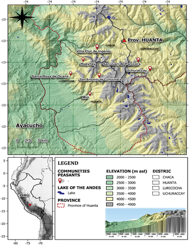
The focus of our analysis is on the Huanta and Luricocha districts in the Province of Huanta, Department of Ayacucho, located in the Central Andes region of Peru between the Apurímac (east) and Mantaro (west) rivers (Figure 1). To evaluate the impact of forced migration due to sociopolitical conflict and subsequent return of the population, we selected seven rural communities for our landscape metrics analysis: (1) Huayllay (3638–4539 m asl); (2) Mio (2738–3786 m asl); (3) San Antonio de Culluchaca (2998–4838 m asl); (4) San Juan de Parccora (3683–4723 m asl); (5) Santa Rosa de Ocana (2594–4349 m asl); (6) Uchuraccay (3708–4908 m asl); and (7) Villa Flor de Ingenio (3451–4490 m asl); in these communities, human migration was more intense during the conflict, which motivates the selection of these areas to conduct the multi-temporal evaluation of land cover. The climate of the Huanta town, as shown by the climogram from the National Service of Meteorology and Hydrology (Figure 1, Appendix; https://www.senamhi.gob.pe), is a Cwb-Temperate climate according to the Köppen classification, characterized by dry winters and mild summers, typical of elevated areas in the Tropical Andes. At present, the biota is distributed across elevational belts, composed of three main ecological zones: the quechua (2300–3500 m asl), the suni (3200–3900 m asl), and the puna, located just below the snowline, which are roughly correlated with the 6°C isotherms of mean annual temperature (Holdridge 1966; Ministerio del Ambiente 2019; Pulgar Vidal 1941; von Humboldt and Bonpland 1805).

Figure 1. Location of study area.

In the studied area, there are ten different land cover types, which are listed in Table 1 and illustrated in Figure 2.

Figure 2. The different land covers identified in the present study. (a) lake; (b) high Andean grassland; (c) forest plantation; (d) wetlands; (e) rocky outcrop; (f) scrubland; (g) bare soil; (h) high Andean scrubland; (i) Croplands; and (j) scrubland of Dodonaea viscosa jacq.

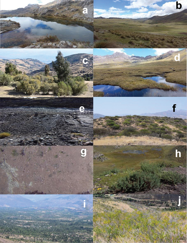
Table 1. List of land cover.

Land cover	Altitude (m asl)	Characteristics
Lakes (A)	3964–4343	Located in small plains surrounded by wetlands and high Andean grasslands, the shores can freeze during the cold seasons.
High Andean grasslands (B)	3500–4650	Or the puna found on almost flat to steep terrains and dominated by high Andean Poaceae, such as Stipa ichu, Calamagrostis sp., Pycnophyllum sp., and Festuca sp., among others (Ministerio del Ambiente 2019).
Forest plantations (C)	3585–3870	Mixed with thickets and high Andean grasslands, grow in rugged terrains, involving species such as Pinus radiata and Eucalyptus globulus.
High Andean Wetlands (D)	3800–4350	Fed by rain and underground waters, with slight contractions during the dry seasons, are located in the bottoms of valleys and near the lagoons, dominated by evergreen hydrophilic herbaceous cushion vegetation, including Distichia muscoides, Plantago rigida, and Werneria caespitosa, among others (Maldonado Fonkén 2014).
Rocky outcrops (E)	4531–4912	Steep slopes previously covered by glaciers at the top of the mountains and covered by scarce to no vegetation (Ministerio del Ambiente 2019).
Scrublands (F)	2214–3800	Located on the border of the high Andean grasslands, are dominated by succulent plants such as Opuntia subulata and Agave americana, as well as shrubs like Mutisia acuminata, Ophryosporus peruvianus, Baccharis tricuneata, and Senna versicolor. Small trees such as Acacia macracantha, Schinus molle, Escallonia resinosa, and Parkinsonia aculeata are also found within this vegetation type (De la Cruz-Arango et al. 2020).
Bare soil (G)	2259–4154	Desert areas eroded by natural or anthropic events.
High Andean scrublands (H)	4000–4500	Forming small communities in contact with the High Andean grasslands and rocky outcrops, are dominated by Parastrephia., Lupinus, Hesperomeles, Locaria., and Senecio, among others (Ministerio del Ambiente 2019).
Croplands (I)	2259–3775 m asl	Mostly of Solanum tuberosum, Zea mays, Pouteria lucuma, Inga edulis, Persea americana, Caesalpinia spinose, among others.
Scrublands of Dodonaea viscosa (J)	3396–3775 m asl	Homogeneous communities of evergreen character and rapid growth, in soils with rugged relief, eroded and disturbed by anthropic action (De la Cruz-Arango et al. 2020).

2.2. Preprocessing

In this study, we selected satellite images of the study areas based on two criteria to ensure the validity and accuracy of our results. Firstly, we chose images with minimal or no cloud cover to minimize the impact of cloudiness on our interpretation of the images. Secondly, we selected images that captured the differentiability of the phenological phases of the plants, specifically during the dry season between May and August (Exavier and Zeilhofer 2021). Through the implementation of these criteria, we ensured that the satellite images used in our study were of high quality and provided a clear representation of the study areas.

2.2.1. Image co-registration

We first performed a manual co-registration of PeruSat-1 images with Sentinel-2 images acquired on close dates for comparison (Table 1). To accomplish this, we used the QGIS software (Usha, Anitha, and Lakshmanan 2012) to georeference the images and employed a polynomial transformation based on control points identifiable in both images. This process allowed us to compare the PeruSat-1 images with the Sentinel-2 images to ensure the validity and accuracy of our results.

Additionally, for multitemporal evaluation, co-registration is a crucial step. To decrease positional errors caused by factors such as sensor focus or rugged terrain, we performed a local co-registration on selected Landsat 5–8 images using the AROSICS library (Scheffler et al. 2017). This process allowed us to accurately compare the different Landsat images over time and to obtain a more precise understanding of the changes that have occurred in the study areas. Overall, the co-registration of satellite images was an important step in ensuring the validity and accuracy of the results obtained in this study.

2.2.2. Radiometric correction

To transform digital levels into actual radiation measured by the sensor and then surface reflectance, we used calibration parameters, which consist of a multiplicative term (gain) and an additive term, specific to the sensor and band through of Dark Objects Subtraction (DOS1) method (Chavez 1996). To apply this algorithm, we used the Semi-Automatic Classification Plugin for QGIS and for Sentinel images (Congedo 2021; Klingseisen, Metternicht, and Paulus 2008) and the RSToolBox for Landsat images (Leutner, Horning, and Schwalb-Willmann 2019). Additionally, we standardized the PeruSat-1 images of surface reflectance with the RSToolBox.

To normalize the co-registered Landsat images, we used the Iteratively Reweighted Multivariate Alteration Detection algorithm (Canty 2019), available through Python notebooks as executable Docker images. This normalization is crucial for detecting changes when comparing images taken under different lighting conditions and at different times.

To enhance the multitemporal classification, we included the elevation and slope variables derived from the Aster GDEM digital elevation model with a 30 m spatial resolution. We filled any missing values with the Fill Sinks function in Saga-GIS (Conrad et al. 2015; H. Wang et al. 2021) to incorporate the effect of topography on the land surface and improve the accuracy of the multitemporal classification. The inclusion of elevation and slope variables, as well as the completion of missing values significantly improved the accuracy of the multitemporal classification results.

2.2.3. Selection of training data for classification and accuracy assessment

During the dry season of July to August in 2020, we surveyed and georeferenced 2605 training and validation sites of representative areas for land cover using a Garmin 67S GPS during field activities (Table 2, Appendix). To increase the photo-interpretation training points, we uploaded the resulting database to the QGIS software (QGIS Development Team 2021) and used high-resolution images to ensure adequate representation and distribution of each type of land cover. Subsequently, we allocated 75% of the baseline data for algorithm training and 25% for the external validation of the accuracy of the results.

Table 2. List of the multispectral images used in the present study.

Source	imagery date	Spectral bands	Spatial resolution	Web address	Reference
PeruSat-1	2017/06/17 2020/08/18 2020/08/18 2020/06/29	Blue: 0.45–0.52 µm Green: 0.53–0.60 µm Red: 0.62–0.69 µm NIR: 0.76–0.89 µm Panchromatic: 0.45–0.75 µm	2.8 m in multispectral 0.7 m in pansharpening	https://www.gob.pe/conida	(CONIDA. Manual Para El Uso de La Plataforma de Atencion al Usuario y Cliente de La CONIDA 2020)
Sentinel-2	2017/05/18 2020/07/01	Blue: 490 nm. Green: 560 nm Red: 665 nm NIR: 842 nm	10 m in multispectral	https://scihub.copernicus.eu/	(COPERNICUS Copernicus Open Access Hub. ESA. 2014)
Landsat-5	1986/01/31 1990/08/06 2000/06/30 2010/07/12	Blue: 450–520 nm Green: 520–600 nm Red: 630–690 nm NIR: 760–900 nm	30 m in multispectral	https://www.usgs.gov/core-science-systems/nli/landsat/	(U. S. Geological Survey Landsat 8: U.S. Geological Survey Fact Sheet 2013-3060 2013)
Landsat-8	2020/08/08

2.3. Classification

We utilized the free software gdal (Rouault et al. 2022) and the Scikit Learn libraries in Python (Pedregosa et al. 2011) for pixel classification and traditional image analysis based on GEOBIA objects. For moderate-resolution images (Landsat 5 and 8) and high-resolution images (Sentinel-2), we employed a pixel-based approach and augmented our training points with new ones obtained from photo-interpretation of freely available high-resolution images.

In contrast, for the very high-resolution PeruSat-1 images, we employed the GEOBIA framework for image segmentation, using spectral features and the open-source library RSGISLib, along with the Operational Large-Scale Segmentation of Imagery Based on Iterative Elimination algorithm (Chen et al. 2018; Shepherd, Bunting, and Dymond 2019). This function uses k-means clustering to group pixels into uniquely labelled geographic regions, reducing the number of regions through an iterative elimination process until reaching a minimum size that corresponds to the smallest unit of the derived mapping products. The final segmentation was achieved by relabelling the recorded regions through sequential numbering.

The algorithm required the specification of two parameters: (1) the initial number of cluster centres (300), and (2) the minimum mapping unit for the elimination process (nine pixels, or 4.41 square meters). The first parameter represents the number of seeds or initial groups in the characteristic space (k), to get an appropriate value of the parameter (k) we iteratively evaluate a list of values (k = 50 to 500, at intervals of 50), while the latter defines the size of the segments.

We assessed the quality of the segmentation through visual evaluation, then vectorized and labelled the segmented images based on the training points. Finally, we calculated the average values of all bands for each segment to perform the classification.

2.3.1. Tuning the machine learning model hyperparameters

We trained a machine learning model for land cover classification using Grid Search, a method that evaluates all combinations of hyperparameters given in the configuration grid (Yang and Shami 2020). We used the Support Vector Machine (SVM) algorithm, a powerful machine learning tool for processing satellite images, that is particularly effective for datasets with small training samples (P. Wang, Fan, and Wang 2021). We adjusted the hyperparameters using a 10-fold cross-validation scheme for each image, evaluating the precision metric with 25% of the original reference dataset obtained during field activities. After selecting the optimized hyperparameters, we applied the best model to the entire image to complete the prediction.

2.3.2. Transition analysis in multitemporal coverage

We generated a Sankey diagram of the land use and land cover (LULC) maps based on Landsat data using the OpenLand package (Exavier and Zeilhofer 2021). The diagram was created by cross-tabulating the classified raster layers, extracting interval levels, category levels, and transition levels. This allowed us to examine and identify the transitions between coverages over time within the evaluated period (Aldwaik and Pontius 2012). The accuracy assessment of these maps was assessed using a stratified random design with the strata defined by the map classes, a sample of 237 points were distributed proportionally to the coverage area and an error matrix was constructed, estimating the error-adjusted land change area with confidence interval and normalized area (Olofsson et al. 2013).

2.3.3. Relationship between land cover and population

We conducted linear regression analysis to evaluate the association between the size of the population and the extent of different land covers. This analysis was based on the number of inhabitants obtained from the national censuses of Peru conducted by the INEI in 1981, 1993, 2007, and 2017 at the district level, which were obtained from the REDATAM database. The aim of the analysis was to determine if the association was positive or negative and to evaluate the significance of the estimated parameters.

2.3.4. Landscape metrics

We utilized the patch matrix model, a useful tool for analysing the interaction between spatial patterns and ecological processes in both natural and anthropogenically modified landscapes (Lausch et al. 2015). When the grain sizes of data differ, re-sampling the finer data to match the coarser grain is often necessary. This is achieved by assigning the category of the smaller cells to the single larger cell, as described in reference (Turner and Gardner 2015a). To align with Landsat spatial resolution, we resampled the highest resolution classified images of land cover (Sentinel) we applied the majority aggregation approach with the R terra package using the aggregate function (Hijmans 2022).

For each community and land cover type from satellite sensors, we calculated the Aggregation index (AI), Edge density area (ED), Mean of Euclidean nearest-neighbour distance (ENN), Contagion, and Shannon Diversity Index using the landscapemetrics library in R (Hesselbarth et al. 2019). These metrics were calculated using an 8 × 8 cell neighbourhood at both the class and landscape levels, respectively.

3. Results and discussion

3.1. The classification process

Our study reliably quantified the coverages in the study area. The average accuracy metric of land cover maps classified with a per-pixel approach using coarse and medium resolution imagery was 88.29% for Landsat multitemporal images, followed by 92.13% for Sentinel images. This accuracy was achieved through the use of training data that incorporated pure pixel samples to provide the necessary information to characterize the classes, in agreement with Foody & Mathur (Foody and Mathur 2006), who obtained an accuracy of 92%.

The use of very high-resolution from PeruSat-1 images (0.7 m) facilitated the identification of smaller coverages, such as fragmented scrublands, small forest plantations, wetlands, and water bodies, through the application of object-based segmentation and image analysis techniques (GEOBIA). This approach resulted in an average accuracy of 87.75% (Table 1, Appendix), which was slightly lower than the pixel-based approach but in line with previous studies reporting accuracies ranging from 83% to 89.64% (Fu et al. 2017). The lower accuracy of 87.75% compared to the 92.13% mean obtained with lower resolution images (10 m) may be due to the smaller number of objects selected as training areas for classification. To address this, Coca-Castro et al (Coca-Castro et al. 2021). increased the number of training points for classification by segmenting 100 objects per evaluation zone.

Our results also support previous studies that the SVM algorithm for classification is appropriate and improves accuracy percentages when using medium to fine resolution images and broad land cover classes (Duro, Franklin, and Dubé 2012). Both object-based and pixel-based classification methods show high and reliable accuracy, with the latter being more accurate in classifying coverages, although more computationally demanding.

We found that the medium resolution pixels did not effectively identify smaller coverages in the study area such as fragmented scrublands, forest plantations, wetlands, and water bodies. Our results suggest that the support vector machine algorithm improved the accuracy in classifying land cover when applied to medium to fine resolution images and broad land cover classes. Both object-based and pixel-based classification methods demonstrated high and reliable accuracy. The pixel-based method was found to be more accurate in classifying coverages, although it requires more computational resources.

3.2. Land cover dynamics

Our analysis revealed that high Andean grasslands and scrub were the predominant land covers in the study area, as shown in Figures 3 and 4. However, these coverages changed over time, but most of the regressions between different land covers and human population size are non-significant correlations (Table 3), although there are visual trends and high coefficient of determination values, generated due to the small amount of data over time. However, it can be an indicator of the dynamics that exist in these Andean zones between ecosystems and society (Figure 2, Appendix). Both high Andean grasslands and scrublands showed a slight decrease over time, attributed to the expansion of cultivated land, due to the return of the population to abandoned lands.

Figure 3. Multitemporal-LandSat verification of land cover types in district the Huanta and Luricocha, province the Huanta, Ayacucho Department, Central Andes of Peru.

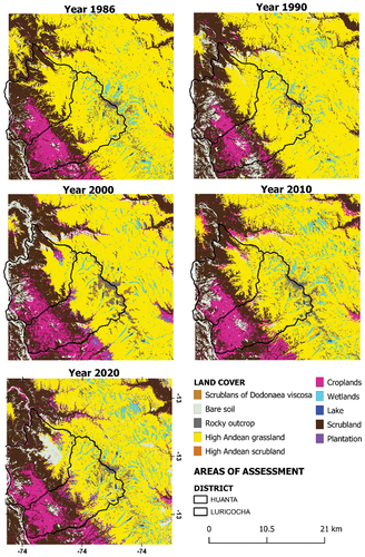
Figure 4. Transition of the land covers in the multitemporal-Landsat images. (ro) rocky outcrop; (we) wetlands; (La) Lake; (HaSL) high Andean scrubland; (FP) forest plantations; (SLD) scrublands of Dodonea viscosa; (Bsl) bare soil; (cr) croplands; (sc) scrublands; and (gr) high Andean grassland.

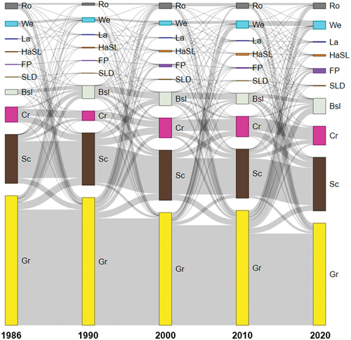
Table 3. Estimated values of the linear regression parameters with their level of significance and coefficient of determination.

Land cover	Huanta			Luricocha
	Parameter	P-value	R2	Parameter	P-value	R2
Croplands	a = 504.038	*	0.99	a	ns	0.63
	b = 0.071	**		b	ns
Forest plantations	a	ns	0.18	a	ns	0.39
	b	ns		b	ns
High Andean grassland	a = 10760.11	*	0.46	a	ns	0.29
	b	ns		b	ns
High Andean scrubland	a	ns	0.02	a	ns	0.12
	b	ns		b	ns
Lake	a	ns	0.33	a	ns	0.62
	b	ns		b	ns
Bare soil	a	ns	0.32	a	ns	0.37
	b	ns		b	ns
Rocky outcrop	a = −457.19	.	0.98	a	ns	0.98
	b = 0.035	**		b = 0.015	**
Scrublands	a = 4597.18	**	0.76	a	ns	0.003
	b	ns		b	ns
Scrublands of Dodonea viscosa	a	ns	0.36	a	ns	0.46
	b	ns		b	ns
Wetlands	a	ns	0.43	a	ns	0.62
	b	ns		b	ns

Notes: a = intercep, b = slope.

Statistical significance : ’ *** ’: p < 0.001; ’ ** ’: p < 0.01; ’ * ’: p < 0.05; ’. ’ : p < 0.1.

ns: not significant.

Prior to this return, it is possible that the vegetation in these areas will recover slightly due to the reduction of human activities. Therefore, the resumption of agricultural and livestock activities results in the transformation of the landscape to adapt it to human needs and consequently influences the decrease of grasslands and scrublands, as illustrated in Figure 4. Research on high Andean grasslands indicates that more than two years are needed for recovery (Mosquera et al. 2022), and fires have the most significant impact on this type of vegetation cover (Bush et al. 2022). However, high Andean grasslands are susceptible to disturbances and can recover quickly depending on the frequency of fires and other human activities (Zomer, Ramsay, and Bernhardt‐Römermann 2021) as observed in Figure 4.

The availability of more labour, favourable conditions for agriculture, and high yields made cultivated land the third most widespread land cover, which increased from the year 2000 and replaced other covers, as the local population progressively returned to the area (Vacquié et al. 2016; Zhang, Li, and Song 2014). Of course, it is reasonable to expect that this interaction between the human population and the surrounding landscape had significant impacts on the ecosystems, causing environmental degradation, threats to ecological diversity, and wildlife (Chabuz et al. 2019; Mansour, Al-Belushi, and Al-Awadhi 2020).

Furthermore, a similar trend is observed in the cases of rocky outcrops, bare soil and forest plantations, coinciding with previous reports that, in the Andes, forest plantations, the overgrazing load and agriculture are spreading and replacing natural environments (Tovar, Seijmonsbergen, and Duivenvoorden 2013), being related to anthropogenic factors and their impact on the dynamics of landscape change (Chabuz et al. 2019). These changes occurred mainly in areas of natural vegetation that may be explained by the magnitudes and directions of interaction of socioeconomic agents and the surrounding environment (Kefalas et al. 2019).

On the other hand, the observed expansion of bare soil increases the risks of soil erosion, potentially worsened by climatic change (Correa et al. 2016), a pattern that has been commonly reported elsewhere in mountainous regions and requires implementation to apply soil conservation technologies (Harden 2001). We found no clear pattern regarding the temporal variation of the area covered by the high Andean wetlands. Effectively, wetlands were almost constant throughout the assessed period, except in 1990 and 2000, probably due to the droughts reported before 2010 (http://www.climatologylab.org) and that there were increases in their coverage in later years, possibly due to the construction of dikes that increased the volume of water in lakes (Figure 4).

However, our results do not agree with the significant and drastic loss of natural environments due to croplands reported in other parts of the Northern Peruvian Andes between 1987 and 2007, that reported a decrease in natural environments of 42.7% (Tovar, Seijmonsbergen, and Duivenvoorden 2013).

Finally, our results contradict our expectations of detecting a vegetation regeneration prompted by the abandonment of the agricultural areas due to the sociopolitical conflicts or the farmers’ shift towards other economically more beneficial activities. Relatively short regeneration timespans of six to ten years were reported for the wetter Northern Andes but only regarding their phytophysiognomy (Sarmiento et al. 2003), that is, insufficient to reach the species richness observed under more pristine conditions. Thus, vegetation regeneration in the dryer conditions of the Central Andes may require longer periods of time. Worse still, the vegetation found in very remote pristine ecosystem relicts of the Peruvian Andes, dominated by newly-described plant species currently extinct in the remnant areas (Sylvester et al. 2017), suggests that regeneration would never reach the maximum possible species richness, unless reintroduction actions are taken.

3.3. Landscape metrics

From the coverage classifications, landscape metrics were extracted based on maps (Figures 3, 5 and 6), we evaluated current patterns based on cover types and describe their structure in a disturbed Andean area, and extracted the Aggregation Index (AI), Edge density area (ED), Mean of Euclidean Nearest-Neighbor distance (ENN); these are indicators to evaluate the configuration of the landscape.

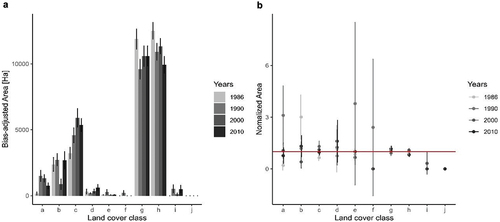
Figure 5. (a) Error-adjusted estimated areas of change and associated 95% confidence intervals for land cover. (b) Error-adjusted normalized areas and confidence intervals scaled by land cover. Rocky outcrops (a), croplands (b), Wetland (c), Lake (d), high andean scrublands (e), scrublands (f), high andean grasslands (g), forest plantations (h), scrublands of dodonaea viscosa (i), bare soil (j).

The maps showed that High Andean grassland, wetlands, scrublands, bare soil, rocky outcrop and forest plantations are the dominant coverages for the study areas; on the other hand, bodies of water (lake), croplands and scrublands of Dodonaea viscosa Jacq. are the most restricted class, all of them at higher altitudes, with reduced areas and too far away from one another.

Figure 5a, shows the area estimated from the error matrix constructed for the years 1986, 1990, 2000 and 2010. The land cover of rocky outcrop, croplands, wetlands, high Andean grassland and forest plantations has greater extension, while lake, high Andean scrubland, scrublands and Dodonea viscosa scrublands have a small area, and the bare soils estimate is zero due to the temporal variation in its spatial distribution.

Therefore, in Figure 5b we reported the relative mapped area of land cover (i.e. the error-adjusted area estimates are divided by the mapped area of each land cover), where

a scaled value of 1.0 (red line) indicates the original mapped area. Therefore, if the confidence intervals (scaled by map area) include the value of 1.0, the mapped area of land cover falls within the confidence interval estimated from the error-adjusted area of land cover, suggesting no significant difference. This is the case for rocky outcrop, croplands, wetlands, lake, high Andean grassland and forest plantations; while the high Andean scrubland, scrublands, Dodonea viscosa scrublands land cover is outside the 95% confidence interval, based on the adjusted area estimate indicating that the difference between the mapped area and the error-adjusted area was substantial. Finally, it was not possible to estimate the confidence interval for the bare soil, due to the dynamics for fires caused by inhabitants dedicated to livestock.

The coverage patterns tend to unify (rocky outcrop and bare soil), with few fragmented areas such as wetlands, high Andean grassland, lake, forest plantation; croplands are more aggregated and the latter three are related to anthropogenic activities. (Figures 2 and 3, Appendix); landscapes that sustain anthropic activities such as croplands lend themselves to being homogeneous areas separated by clear boundaries (Lausch et al. 2015).

There is also a clear difference when obtaining the Aggregation index (AI) from different image resolutions; showing that the landscape is heterogeneous and there are no major differences between each studied community (Figure 6 and 7, Appendix).

The ED for High Andean grassland indicates high values in each community and interact with wetlands, bare soil, rocky outcrop and scrublands, showing that they are dense landscapes, are interrelated and dominate the landscape.

The most fragmented coverages, such as croplands, High Andean scrubland, forest plantations are dispersed and not connected.

Areas with lakes are the weakest in terms of ED, insufficient from an ecological point of view (Figure 4, Appendix). But there are differences in evaluating ED, based on values derived from images with varying resolutions, so it is important to create updated land cover maps using higher-resolution imagery (Sertel et al. 2018).

With regard to the ENN, the results indicate that lakes are the most isolated, which is a distinctive feature of the high Andean zones.

For croplands, this coverage is hardly detectable in higher altitude zones, owing to the gradual process of human settlement in sloped areas, in accordance with Huang et al., (2022) (Huang et al. 2022) who mention that intensive land use changes only occur in flat areas and the transition of land cover changes and landscape patterns in mountainous areas are different from those in low altitude areas.

This study shows that the landscape pattern in the high Andean zones shows unique characteristics where there are still areas with natural environments to be preserved, being High Andean scrubland y wetlands.

Also, High Andean grassland is the coverage with the greatest spatial distribution, which is why it has lowest degree of isolation. On the other hand, the analysis reveals that land cover forest plantation and High Andean scrubland are isolated and show greater dispersion (Figure 3) and (Figure 6 and 7, Appendix).

As grain size increases (i.e. resolution decreases), cover types that are rare on the landscape typically become less well represented or may even disappear (Turner and Gardner 2015b), which directly influences the calculation of the Shannon biodiversity index, being more noticeable in Landsat shown in the Table 4.

Table 4. Landscape metrics.

COMUNNITY	PERUSAT	SENTINEL	LANDSAT
OCCANA
Aggregation index	97.5	81.8	88.7
Contagion	68.7	50.8	72.1
Shannon Diversity Index	1.16	1.36	0.782
UCHURACCAY
Aggregation index	98	88.5	88.9
Contagion	71.9	66.9	72.2
Shannon Diversity Index	1.05	0.943	0.818
MIO
Aggregation index	92.5	65.4	65.8
Contagion	49	31.7	35.8
Shannon Diversity Index	1.75	1.71	1.47
VILLA FLOR DE INGENIO
Índice de agregación	97.3	83.2	87.9
Contagion	71.3	55.4	76.7
Shannon Diversity Index	1.05	1.14	0.632
CUYUCHACA
Aggregation index	98.1	91.1	87.4
Contagion	69.8	71.8	72.4
Shannon Diversity Index	1.27	0.872	0.803
HUAYLLAY
Aggregation index	98	77.8	82.3
Contagion	66.1	47	64.1
Shannon Diversity Index	1.2	1.33	1.04
PARCCORA
Aggregation index	96.6	84.8	85.5
Contagion	65	58.7	71.1
Shannon Diversity Index	1.28	1.16	0.832

3.3. Final remarks

In general, changes generated by anthropic factors to natural areas result in small and isolated vegetation patches, affecting the services provided by the environments (Kanianska 2016). This situation is of particular concern in the Central Andes, where habitat alteration affects water supply (Tovar, Seijmonsbergen, and Duivenvoorden 2013). Thus, although Huanta and surroundings has been referred to as a medium conservation priority (Supplementary material from Brooks et al. 2006) (Madrigal-Martínez and Miralles i García 2019), the habitat transformations observed and previously found by Madrigal-Martínez and Miralles i García [84] to be deeper and more extended compared to those of the remnant Central Andean highlands, strongly appeals for a bigger concern regarding this underexplored enclave within a world’s biodiversity hotspot.

4. Conclusions

For 34 years, grassland and scrubland cover has had a steeper decline compared to other covers. Recently, forest plantations have increased at the expense of natural areas. In addition, conflicting historical events that occurred between 1986 and 2000, caused the temporary migration of the population, which resulted in a slight increase in the coverage of grasslands and scrublands after being altered mainly by agricultural and livestock activities. Moreover, the gradual return of the population to their lands affected areas that were beginning to recover. Thus, we may say that the high Andean ecosystems have a slow process of regeneration. This observation would serve as a starting point for future studies on the conservation and restoration of high Andean ecosystems.

High resolution images allow for the detection of small surface land covers and provide more accurate estimates of the actual area, directly influencing the values of the extracted metrics. In contrast, medium resolution images exhibit greater similarity among the values.

Author contributions

1. Marco Arizapana Almonacid: conceptualization, software, fieldwork, writing-original draft preparation, writing-review and editing, supervision, project administration and funding acquisition.

2. Victor Henry Pariona Antonio: methodology, software, validation, data analysis, fieldwork, writing-original draft preparation and writing-review and editing.

3. Italo Castañeda-Tinco: conceptualization, methodology, software, validation, data analysis, fieldwork, writing-original draft preparation and writing-review and editing.

4. Julio Cesar Ascención Mendoza: methodology, software, validation, data analysis, fieldwork, writing-original draft preparation and writing-review and editing.

5. Edgar Gutiérrez Gómez: methodology,writing-original draft preparation and writing-review and editing.

6. Paolo Ramoni-Perazzi: validation, writing-original draft preparation, writing-review and editing and supervision.

Acknowledgements

To the National Commission for Aerospace Research and Development (CONIDA) for facilitating access to the earth observation images captured by the Peruvian satellite PeruSAT-1 and to the company Robotic Air Systems for the collaborative work with the research group, training and for providing the high performance industrial RPAS system for the high Andean zones.

Disclosure statement

The authors does not have conflict of interest; all authors have read and agreed to the published version of the manuscript.

Supplementary material

Supplemental data for this article can be accessed online at https://doi.org/10.1080/19475683.2024.2304203.

Additional information

Funding

This work was supported by the mining canon (002-2019-P.CO-UNAH/FOCAM).

Notes on contributors

Marco Aurelio Arizapana-Almonacid

Marco Arizapana Almonacid (M.A.A.A.) Graduated in Animal Husbandry and Forestry Engineering from Universidad Nacional del Centro del Perú, Master in Forest Resources from Universidade de São Paulo – Brazil. PhD in Forest Ecology – Universidade Federal de Lavras – Brazil. Experience in Mountain Forest Ecology and Plant Anatomy. Currently professor of Ecology and Dasometry at Universidad Nacional Autónoma de Huanta.

Victor Henry Pariona-Antonio

Victor Pariona (V.H.P.A.) Researcher at the Remote Sensing and Mountain Ecology Research Center, Universidad Autónoma de Huanta, Ayacucho; Graduate in Forestry and Environmental Sciences from Universidad Nacional del Centro del Perú.

Italo Castañeda-Tinco

Italo Castañeda-Tinco Researcher at the Remote Sensing and Mountain Ecology Research Center, Universidad Autónoma de Huanta, Ayacucho; Graduate in Forestry and Environmental Sciences from Universidad Nacional del Centro del Perú.

Julio Cesar Ascención Mendoza

Julio Cesar Ascención Mendoza (J.C.A.M.) Researcher at the Remote Sensing and Mountain Ecology Research Center, Universidad Autónoma de Huanta, Ayacucho; Graduate in Forestry and Environmental Sciences from Universidad Nacional del Centro del Perú.

Edgar Gutiérrez Gómez

Edgar Gutiérrez Gómez (E.G.G.) Doctor in Education Sciences, National University of Education Post-doctorate in Education, National University of Education. Master in University Teaching, National University of San Cristobal de Huamanga. Bachelor in Education Sciences, Universidad Nacional de San Cristóbal de Huamanga.

Paolo Ramoni-Perazzi

Paolo Ramoni-Perazzi (P.R.P) Researcher at the Remote Sensing and Mountain Ecology Research Center, Universidad Autónoma de Huanta, Ayacucho. Also attached to the Applied Zoology Laboratory and the Simulation and Modeling Center of the Universidad de Los Andes, Mérida, Venezuela. B.Sc. in Biology (Universidad de Los Andes, Facultad de Ciencias, Venezuela), M.Sc. in Systematics (Instituto de Ecología AC, México).

References

- COPERNICUS Copernicus Open Access Hub. ESA. 2014.
- Aldwaik, S. Z., and R. G. Pontius. 2012. “Intensity Analysis to Unify Measurements of Size and Stationarity of Land Changes by Interval, Category, and Transition.” Landscape and Urban Planning 106:103–114. https://doi.org/10.1016/j.landurbplan.2012.02.010.
- Anthelme, F., D. Jacobsen, P. Macek, R. I. Meneses, P. Moret, S. Beck, and O. Dangles. 2014. “Biodiversity Patterns and Continental Insularity in the Tropical High Andes.” Arctic Antarctic and Alpine Research 46 (4): 811–828. https://doi.org/10.1657/1938-4246-46.4.811.
- Ball, P.; J. Asher; D. Sulmont; D. Manrique How Many Peruvians Have Died? An Estimate of the Total Number of Victims Killed or Disappeared in the Armed Internal Conflict Between 1980 and 2000; AAAS. Report to the Peruvian Truth and Reconciliation Commission (CVR); American Association for the Advancement of Science: Washington, DC, 2003;
- Baumann, M., and T. Kuemmerle. 2016. “The Impacts of Warfare and Armed Conflict on Land Systems.” Journal of Land Use Science 11 (6): 672–688. https://doi.org/10.1080/1747423X.2016.1241317.
- Bautista-Cespedes, O. V., L. Willemen, A. Castro-Nunez, and T. A. Groen. 2021. “The Effects of Armed Conflict on Forest Cover Changes Across Temporal and Spatial Scales in the Colombian Amazon.” Regional Environmental Change 21 (3). https://doi.org/10.1007/s10113-021-01770-6.
- Berhe, A. A., and J. Males. 2022. “On the Relationship of Armed Conflicts with Climate Change.” PLOS Climate 1 (6): e0000038. https://doi.org/10.1371/journal.pclm.0000038.
- Brooks, T. M., R. A. Mittermeier, G. A. B. Fonseca da, J. Gerlach, M. Hoffmann, J. F. Lamoreux, C. G. Mittermeier, J. D. Pilgrim, and A. S. L. Rodrigues. 2006. “Global Biodiversity Conservation Priorities.” Science 313 (5783): 58–61. https://doi.org/10.1126/science.1127609.
- Brush, S. B. 1982. “The Natural and Human Environment of the Central Andes.” Mountain Research and Development 2:19–38. https://doi.org/10.2307/3672931.
- Buchner, J., V. Butsic, H. Yin, T. Kuemmerle, M. Baumann, N. Zazanashvili, J. Stapp, and V. C. Radeloff. 2022. “Localized versus Wide-Ranging Effects of the Post-Soviet Wars in the Caucasus on Agricultural Abandonment.” Global Environmental Change 76:102580. https://doi.org/10.1016/j.gloenvcha.2022.102580.
- Burgess, R., E. Miguel, and C. Stanton. 2015. “War and Deforestation in Sierra Leone.” Environmental Research Letters 10 (9): 095014. https://doi.org/10.1088/1748-9326/10/9/095014.
- Bush, M. B., A. Rozas-Davila, M. Raczka, M. Nascimento, B. Valencia, R. K. Sales, C. N. H. McMichael, and W. D. Gosling. 2022. “A Palaeoecological Perspective on the Transformation of the Tropical Andes by Early Human Activity.” Philosophical Transactions of the Royal Society B: Biological Sciences 377 (1849): 20200497. https://doi.org/10.1098/rstb.2020.0497.
- Canty, M. J. 2019. Image Analysis, Classification, and Change Detection in Remote Sensing: With Algorithms for Python. 4th ed. Boca Raton: CRC Press.
- Chabuz, W., M. Kulik, W. Sawicka-Zugaj, P. Żółkiewski, M. Warda, M. Pluta, A. Lipiec, A. Bochniak, and J. Zdulski. 2019. “Impact of the Type of Use of Permanent Grasslands Areas in Mountainous Regions on the Floristic Diversity of Habitats and Animal Welfare.” Global Ecology and Conservation 19:e00629. https://doi.org/10.1016/j.gecco.2019.e00629.
- Chavez, P. 1996. “Image-Based Atmospheric Corrections - Revisited and Improved.” Photogrammetric Engineering and Remote Sensing 62 (9): 1025–1036. https://static1.1.sqspcdn.com/static/f/891472/15133582/1321370214637/Chavez_P.S._1996.pdf.
- Chen, G., Q. Weng, G. J. Hay, and Y. He. 2018. “Geographic Object-Based Image Analysis (GEOBIA): Emerging Trends and Future Opportunities.” GIScience & Remote Sensing 55:159–182. https://doi.org/10.1080/15481603.2018.1426092.
- Coca-Castro, A., M. A. Zaraza-Aguilera, Y. T. Benavides-Miranda, Y. M. Montilla-Montilla, H. B. Posada-Fandiño, A. L. Avendaño- Gómez, H. A. Hernández-Hamon, S. C. Garzón-Martínez, and C. A. Franco-Prieto. 2021. “Evaluación de Algoritmos de Clasificación En La Plataforma Google Earth Engine Para La Identificación y Detección de Cambios de Construcciones Rurales y Periurbanas a Partir de Imágenes de Alta Resolución.” Revista de Teledetección 58 (58): 71– 88. https://doi.org/10.4995/raet.2021.15026.
- Congedo, L. 2021. “Semi-Automatic Classification Plugin: A Python Tool for the Download and Processing of Remote Sensing Images in QGIS.” The Journal of Open Source Software 6:3172. https://doi.org/10.21105/joss.03172.
- CONIDA. 2020. “Manual Para El Uso de La Plataforma de Atencion al Usuario yCliente de La CONIDA.” https://www.gob.pe/institucion/conida/informes-publicaciones/1254760-manual-para-el-uso-de-la-plataforma-de-atencion-al-usuario-y-cliente-de-la-conida.
- Conrad, O., B. Bechtel, M. Bock, H. Dietrich, E. Fischer, L. Gerlitz, J. Wehberg, V. Wichmann, and J. Böhner. 2015. “System for Automated Geoscientific Analyses (SAGA) V. 2.1.4.” Geoscientific Model Development 8:1991–2007. https://doi.org/10.5194/gmd-8-1991-2015.
- Correa, S. W., C. R. Mello, S. C. Chou, N. Curi, and L. D. Norton. 2016. “Soil Erosion Risk Associated with Climate Change at Mantaro River Basin, Peruvian Andes.” Catena 147:110–124. https://doi.org/10.1016/j.catena.2016.07.003.
- De la Cruz-Arango, J., J. Gómez-Carrión, M. Chanco-Estela, E. P. Carrillo-Fuentes, and L. Aucasime-Medina. 2020. “Flora y vegetación de la provincia de Huamanga (Ayacucho-Perú).” Journal of the Selva Andina Biosphere 8 (1): 3–18. https://doi.org/10.36610/j.jsab.2020.080100003.
- Duro, D. C., S. E. Franklin, and M. G. Dubé. 2012. “A Comparison of Pixel-Based and Object-Based Image Analysis with Selected Machine Learning Algorithms for the Classification of Agricultural Landscapes Using SPOT-5 HRG Imagery.” Remote Sensing of Environment 118:259–272. https://doi.org/10.1016/j.rse.2011.11.020.
- Enaruvbe, G. O., K. M. Keculah, G. O. Atedhor, and A. O. Osewole. 2019. “Armed Conflict and Mining Induced Land-Use Transition in Northern Nimba County, Liberia.” Global Ecology and Conservation 17:e00597. https://doi.org/10.1016/j.gecco.2019.e00597.
- Exavier, R., and P. Zeilhofer. 2021. “OpenLand: Software for Quantitative Analysis and Visualization of Land Use and Cover Change.” The R Journal 12 (2): 359. https://doi.org/10.32614/RJ-2021-021.
- Figueroa, A. 1984. Capitalist Development and the Peasant Economy in Peru. Cambridge Latin American Studies: Cambridge University Press. https://doi.org/10.1017/CBO9780511759567.
- Foody, G. M., and A. Mathur. 2006. “The Use of Small Training Sets Containing Mixed Pixels for Accurate Hard Image Classification: Training on Mixed Spectral Responses for Classification by a SVM.” Remote Sensing of Environment 103 (2): 179–189. https://doi.org/10.1016/j.rse.2006.04.001.
- Fu, B., Y. Wang, A. Campbell, Y. Li, B. Zhang, S. Yin, Z. Xing, and X. Jin. 2017. “Comparison of Object-Based and Pixel-Based Random Forest Algorithm for Wetland Vegetation Mapping Using High Spatial Resolution GF-1 and SAR Data.” Ecological Indicators 73:105–117. https://doi.org/10.1016/j.ecolind.2016.09.029.
- Gaynor, K. M., K. J. Fiorella, G. H. Gregory, D. J. Kurz, K. L. Seto, L. S. Withey, and J. S. Brashares. 2016. “War and Wildlife: Linking Armed Conflict to Conservation.” Frontiers in Ecology and the Environment 14 (10): 533–542. https://doi.org/10.1002/fee.1433.
- Grima, N., and S. J. Singh. 2019. “How the End of Armed Conflicts Influence Forest Cover and Subsequently Ecosystem Services Provision? An Analysis of Four Case Studies in Biodiversity Hotspots.” Land Use Policy 81 ( August 2018): 267–275. https://doi.org/10.1016/j.landusepol.2018.10.056.
- Harden, C. P. 2001. “Soil Erosion and Sustainable Mountain Development.” Mountain Research and Development 21:77–83. https://doi.org/10.1659/0276-4741(2001)021[0077:SEASMD]2.0.CO;2.
- Hesselbarth, M. H. K., M. Sciaini, K. A. With, K. Wiegand, and J. Nowosad. 2019. “Landscapemetrics: An open-source R tool to calculate landscape metrics.” Ecography 42 (10): 1648–1657. https://doi.org/10.1111/ecog.04617.
- Higazi, A. 2022. “Boko Haram: The Impacts of Insurgency on Pastoralists and Farmers.” Afrique Contemporaine 274 (2): 163–169. https://doi.org/10.3917/afco1.274.0163.
- Hijmans, R. J. 2022. Terra: Spatial Data Analysis. https://cran.r-project.org/package=terra.
- Holdridge, L. R. 1966. Life Zone Ecology. San Jose, Costa Rica: Tropical Science Center. https://reddcr.go.cr/sites/default/files/centro-de-documentacion/holdridge_1966_-_life_zone_ecology.pdf.
- Huang, M., Y. Li, C. Ran, and M. Li. 2022. “Dynamic Changes and Transitions of Agricultural Landscape Patterns in Mountainous Areas: A Case Study from the Hinterland of the Three Gorges Reservoir Area.” Journal of Geographical Sciences 32 (6): 1039–1058. https://doi.org/10.1007/s11442-022-1984-7.
- Hutter, C. R., S. M. Lambert, and J. J. Wiens. 2017. “Rapid Diversification and Time Explain Amphibian Richness at Different Scales in the Tropical Andes, Earth’s Most Biodiverse Hotspot.” The American Naturalist 190:828–843. https://doi.org/10.1086/694319.
- Kanianska, R. 2016. “Agriculture and Its Impact on Land‐Use, Environment, and Ecosystem Services.” In Landscape Ecology, edited by A. Almusaed, 3–26. Rijeka: IntechOpen.
- Kefalas, G., S. Kalogirou, K. Poirazidis, and R. S. Lorilla. 2019. “Landscape Transition in Mediterranean Islands: The Case of Ionian Islands, Greece 1985–2015.” Landscape and Urban Planning 191:103641. https://doi.org/10.1016/j.landurbplan.2019.103641.
- Klingseisen, B., G. Metternicht, and G. Paulus. 2008. “Geomorphometric Landscape Analysis Using a Semi-Automated GIS-Approach.” Environmental Modelling & Software 23:109–121. https://doi.org/10.1016/j.envsoft.2007.05.007.
- Lausch, A., T. Blaschke, D. Haase, F. Herzog, R.-U. Syrbe, L. Tischendorf, and U. Walz. 2015. “Understanding and Quantifying Landscape Structure – a Review on Relevant Process Characteristics, Data Models and Landscape Metrics.” Ecological Modelling 295:31–41. https://doi.org/10.1016/j.ecolmodel.2014.08.018.
- Leutner, B., N. Horning, and J. Schwalb-Willmann. 2019. V. 0.2. Paquete R versión 0.2: RStoolbox: tools for remote sensing data analysis. https://bleutner.github.io/RStoolbox/.
- Madrigal-Martínez, S., and J. L. Miralles i García. 2019. “Land-Change Dynamics and Ecosystem Service Trends across the Central High-Andean Puna.” Scientific Reports 9:9688. https://doi.org/10.1038/s41598-019-46205-9.
- Maldonado Fonkén, M. S. 2014. “An Introduction to the Bofedales of the Peruvian High Andes.” Mires and Peat 15 (5): 1–13. http://mires-and-peat.net/media/map15/map_15_05.pdf.
- Malhi, Y., J. Franklin, N. Seddon, M. Solan, M. G. Turner, C. B. Field, and N. Knowlton. 2020. “Climate Change and Ecosystems: Threats, Opportunities and Solutions.” Philosophical Transactions of the Royal Society B: Biological Sciences 375:20190104. https://doi.org/10.1098/rstb.2019.0104.
- Mansour, S., M. Al-Belushi, and T. Al-Awadhi. 2020. “Monitoring Land Use and Land Cover Changes in the Mountainous Cities of Oman Using GIS and CA-Markov Modelling Techniques.” Land Use Policy 91:104414. https://doi.org/10.1016/j.landusepol.2019.104414.
- McNeely, J. A. 2003. “Conserving Forest Biodiversity in Times of Violent Conflict.” Oryx 37 (2): 142–152. https://doi.org/10.1017/S0030605303000334.
- Ministerio del Ambiente. 2019. MINAM Mapa Nacional de Ecosistemas Del Perú - Memoria Descriptiva. Lima: NEGRAPATA S.A.C.
- Mittermeier, R. A., W. R. Turner, F. W. Larsen, T. M. Brooks, and C. Gascon. 2011. “Global Biodiversity Conservation: The Critical Role of Hotspots.” In Biodiversity Hotspots: Distribution and Protection of Conservation Priority Areas, edited by F. E. Zachos and J. C. Habel, 3–22. Berlin Heidelberg: Berlin, Heidelberg: Springer. ISBN 978-3-642-20992-5.
- Mosquera, G. M., F. Marín, M. Stern, V. Bonnesoeur, B. F. Ochoa-Tocachi, F. Román-Dañobeytia, and P. Crespo. 2022. “Progress in Understanding the Hydrology of High-Elevation Andean Grasslands Under Changing Land Use.” Science of the Total Environment 804:150112. https://doi.org/10.1016/j.scitotenv.2021.150112.
- Murillo-Sandoval, P. J., N. Clerici, and C. Correa-Ayram. 2022a. “Rapid Loss in Landscape Connectivity After the Peace Agreement in the Andes-Amazon Region.” Global Ecology and Conservation 38:e02205. November 2021. https://doi.org/10.1016/j.gecco.2022.e02205.
- Murillo-Sandoval, P. J., N. Clerici, and C. Correa-Ayram. 2022b. “Rapid Loss in Landscape Connectivity After the Peace Agreement in the Andes-Amazon Region.” Global Ecology and Conservation 2022:e02205. https://doi.org/10.1016/j.gecco.2022.e02205.
- Murillo-Sandoval, P. J., K. Van Dexter, J. Van Den Hoek, D. Wrathall, and R. Kennedy. 2020. “The End of Gunpoint Conservation: Forest Disturbance After the Colombian Peace Agreement.” Environmental Research Letters 15 (3): 034033. https://doi.org/10.1088/1748-9326/ab6ae3.
- Oelschlegel, A. 2003. “Informe Final de La Comisión de La Verdad y Reconciliacion En El Perú. Un resumen crítico respecto a los avances de sus recomendaciones.” UNAM - México.https://www.corteidh.or.cr/tablas/r08047-26.pdf.
- Olofsson, P., G. M. Foody, S. V. Stehman, and C. E. Woodcock. 2013. “Making Better Use of Accuracy Data in Land Change Studies: Estimating Accuracy and Area and Quantifying Uncertainty Using Stratified Estimation.” Remote Sensing of Environment 129:122–131. https://doi.org/10.1016/j.rse.2012.10.031.
- Pedregosa, F., G. Varoquaux, A. Gramfort, V. Michel, B. Thirion, O. Grisel, M. Blondel, et al. 2011. “Scikit-Learn: Machine Learning in Python.” Journal of Machine Learning Research 12 (85): 2825–2830.
- Pulgar Vidal, J. 1941. “Las Ocho Regiones Naturales Del Perú.” Museo de Historia Natural ”Javier Prado” Perú: Geografía Del Perú. https://museohn.unmsm.edu.pe/docs/boletines/volumen17.pdf.
- QGIS Development Team. 2021. QGIS Geographic Information System. Borneo: Open Source Geospatial Foundation.
- Rouault, E., F. Warmerdam, K. Schwehr, A. Kiselev, H. Butler, M. Łoskot, T. Szekeres, et al. 2022. “Zenodo.” GDAL 3 (51) https://doi.org/10.5281/ZENODO.5884351.
- Särkinen, T., R. T. Pennington, M. Lavin, M. F. Simon, and C. E. Hughes. 2011. “Evolutionary Islands in the Andes: Persistence and Isolation Explain High Endemism in Andean Dry Tropical Forests.” Journal of Biogeography 39 (5): 884–900. https://doi.org/10.1111/j.1365-2699.2011.02644.x.
- Sarmiento, L., L. Llambí, A. Escalona, and N. Marquez. 2003. “Vegetation Patterns, Regeneration Rates and Divergence in an Old-Field Succession of the High Tropical Andes.” Plant Ecology 166 (1): 145–156. https://doi.org/10.1023/A:1023262724696.
- Scheffler, D., A. Hollstein, H. Diedrich, K. Segl, and P. Hostert. 2017. “AROSICS: An Automated and Robust Open-Source Image Co-Registration Software for Multi-Sensor Satellite Data.” Remote Sensing 9 (7): 676. https://doi.org/10.3390/rs9070676.
- SEPIA, M. 2002. “Nacional sobre desplazamiento Balance Del Proceso de Desplazamiento Por Violencia Política En El Perú (1980-1997).” Amérique Latine Histoire et Mémoire 5:1–14. https://doi.org/10.4000/alhim.647.
- Sertel, E., R. Topaloğlu, B. Şallı, I. Yay Algan, and G. Aksu. 2018. “Comparison of Landscape Metrics for Three Different Level Land Cover/Land Use Maps.” ISPRS International Journal of Geo-Information 7 (10): 408. https://doi.org/10.3390/ijgi7100408.
- Shepherd, J. D., P. Bunting, and J. R. Dymond. 2019. “Operational Large-Scale Segmentation of Imagery Based on Iterative Elimination.” Remote Sensing 11 (6): 658. https://doi.org/10.3390/rs11060658.
- Sylvester, S. P., F. Heitkamp, M. D. P. V. Sylvester, H. F. Jungkunst, H. J. M. Sipman, J. M. Toivonen, C. A. Gonzales Inca, J. C. Ospina, and M. Kessler. 2017. “Relict High-Andean Ecosystems Challenge Our Concepts of Naturalness and Human Impact.” Scientific Reports 7 (1): 3334. https://doi.org/10.1038/s41598-017-03500-7.
- Tilman, D., F. Isbell, and J. M. Cowles. 2014. “Biodiversity and Ecosystem Functioning.” Annual Review of Ecology, Evolution, and Systematics 45:471–493. https://doi.org/10.1146/annurev-ecolsys-120213-091917.
- Tovar, C., A. C. Seijmonsbergen, and J. F. Duivenvoorden. 2013. “Monitoring Land Use and Land Cover Change in Mountain Regions: An Example in the Jalca Grasslands of the Peruvian Andes.” Landscape and Urban Planning 112:40–49. https://doi.org/10.1016/j.landurbplan.2012.12.003.
- Turner, M. G., and R. H. Gardner. 2015a. Landscape Ecology in Theory and Practice. Springer New York. https://doi.org/10.1007/978-1-4939-2794-4.
- Turner, M. G., and R. H. Gardner. 2015b. Landscape Ecology in Theory and Practice: Pattern and Process. Springer New York. https://doi.org/10.1007/978-1-4939-2794-4.
- U. S. Geological Survey Landsat 8: U.S. Geological Survey Fact Sheet 2013-3060 2013.
- Usha, M., K. Anitha, and I. Lakshmanan. 2012. “Landuse Change Detection Through Image Processing and Remote Sensing Approach: A Case Study of Palladam Taluk, Tamil Nadu.” International Journal of Engineering Research and Applications 2 (4): 289–294. https://www.ijera.com/papers/Vol2_issue4/AR24289294.pdf.
- Vacquié, L. A., T. Houet, D. Sheeren, N. de Munnik, V. Roussel, and J. Waddle. 2016. “Adapting Grazing Practices to Limit the Reforestation of Mountainous Summer Pastures: A Process-Based Approach.” Environmental Modelling & Software 84:395–411. https://doi.org/10.1016/j.envsoft.2016.05.006.
- von Humboldt, A.; A. Bonpland Essai Sur La Géographie Des Plantes: Accompagné d’un Tableau Physique Des Régions Équinoxiales, Fondé Sur Des Mesures Exécutées, Depuis Le Dixième Degré de Latitude Boréale Jusqu’au Dixième Degré de Latitude Australe, Pendant Les Années 1799, 1800, 1801, 1802 et 1803; Chez Levrault, Schoell et compagnie, libraires, 1805.
- Wang, P., E. Fan, and P. Wang. 2021. “Comparative Analysis of Image Classification Algorithms Based on Traditional Machine Learning and Deep Learning.” Pattern Recognition Letters 141:61–67. https://doi.org/10.1016/j.patrec.2020.07.042.
- Wang, H., L. Zhang, K. Yin, H. Luo, and J. Li. 2021. “Landslide Identification Using Machine Learning.” Geoscience Frontiers 12:351–364. https://doi.org/10.1016/j.gsf.2020.02.012.
- Yang, L., and A. Shami. 2020. “On Hyperparameter Optimization of Machine Learning Algorithms: Theory and Practice.” Neurocomputing 415:295–316. https://doi.org/10.1016/j.neucom.2020.07.061.
- Yin, H., V. Butsic, J. Buchner, T. Kuemmerle, A. V. Prishchepov, M. Baumann, E. V. Bragina, H. Sayadyan, and V. C. Radeloff. 2019. “Agricultural Abandonment and Re-Cultivation During and After the Chechen Wars in the Northern Caucasus.” Global Environmental Change 55 ( January): 149–159. https://doi.org/10.1016/j.gloenvcha.2019.01.005.
- Young, K. R. 2009. “Andean Land Use and Biodiversity: Humanized Landscapes in a Time of Change.” Annals of the Missouri Botanical Garden Missouri Botanical Garden 96:492–507. https://doi.org/10.3417/2008035.
- Zhang, Y., X. Li, and W. Song. 2014. “Determinants of Cropland Abandonment at the Parcel, Household and Village Levels in Mountain Areas of China: A Multi-Level Analysis.” Land Use Policy 41:186–192. https://doi.org/10.1016/j.landusepol.2014.05.011.
- Zomer, M. A., P. M. Ramsay, and M. Bernhardt‐Römermann. 2021. “Post‐Fire Changes in Plant Growth Form Composition and Diversity in Andean Páramo Grassland.” Applied Vegetation Science 24 (1). https://doi.org/10.1111/avsc.12554.