Rapid monitoring of the spatial distribution of soil organic matter using unmanned aerial vehicle imaging spectroscopy

ABSTRACT

An existing technique for quickly obtaining the spatial distribution data of soil organic matter (SOM) involves combining an unmanned aerial vehicle (UAV) platform and imaging spectroscopy technology; this technique is suitable for precision agricultural management and real-time monitoring. In this study, the average spectral data were first extracted via circular regions of interest (ROIs) of different radii and modelled using the measured SOM to determine the optimal extraction range for the spectral data. Partial least-squares regression (PLSR) and support vector machine (SVM) models were constructed based on the raw spectra, standard normal transform spectra, multiple scattering-corrected spectra, and first-order differential spectra. The difference index, ratio index, and normalized index were calculated and analysed for their correlation with SOM content, and the spectral indices were screened to establish the SOM prediction model. Finally, the accuracy of the model was evaluated, and we selected the optimal model to map the spatial distribution of SOM. The results of our study show that 1) the radius of the ROI significantly affects the model’s accuracy; 2) the accuracy of the nonlinear SVM model is much higher than that of the linear PLSR model; 3) the prediction model based on spectral indices is better than full-band model. This study can serve as a model for the application of UAV imaging spectroscopy technology to field-scale SOM estimations and rapid monitoring, as well as provide technical support for precision agriculture and climate change studies.

KEYWORDS:

• UAV
• imaging spectroscopy
• spectral index
• coastal soil
• soil organic matter

1. Introduction

Soil organic matter (SOM) comprises carbonaceous organic compounds found in the soil. These compounds are an active component of the soil and play a critical role in soil formation, soil fertility, environmental protection, and sustainable agricultural development (Jin et al. 2017). Therefore, there is an urgent need for the high-resolution and high-precision rapid monitoring of the spatial distribution characteristics of SOM at the field scale for precision agricultural management. Traditionally, SOM content is mainly determined by manually sampling the field and using chemical determination methods, which are time-consuming, inefficient, and can only determine the SOM content at the sampling point, making it difficult to carry out large-scale and multi-frequency SOM monitoring. In recent years, based on the response relationship between the soil spectral reflectance and SOM content, visible-near-infrared hyperspectral technology has been widely used in the investigation of SOM content (Angelopoulou et al. 2019), and many researchers have used reflectance spectrometry to develop soil hyperspectral technology as a routine means of quantifying SOM (Cao and Yang 2023; Chen et al. 2021; Pärnpuu et al. 2022; Tang et al. 2021; Xiao et al. 2023; G. H. Zheng et al. 2016). However, reflectance spectrometry can only obtain SOM information from point-like soil samples, meaning that it struggles to meet the need for rapid access to the spatial distribution of SOM in the context of precision agriculture (J. K. Biney et al. 2021).

Unmanned aerial vehicles (UAVs) have the advantages of mobility and flexibility; using their various sensors, they can obtain regional-scale data in a rapid and real-time manner, and they have therefore been widely used in the spatial investigation of land resources in recent years. Numerous researchers have used UAV imaging spectral systems to conduct research on a range of agricultural matters, including the monitoring of vegetation growth, pest and disease detection, yield estimations, and feature classification and identification (Heil, Jörges, and Stumpe 2022; Perz and Wronowski 2018; Shanmugapriya et al. 2019; Sun et al. 2018). In recent years, this technique has also been widely used in soil attribute surveys. Aldana-Jague et al. (2016) used a small UAV equipped with a multispectral camera to perform soil organic carbon (SOC) inversion in the bare soil of farmland, demonstrating the feasibility of using an organic combination of UAV platforms and soil spectral data to predict and map soil properties. J. Zhou et al. (2023) collected centimetre-level resolution multispectral images using a UAV and mapped the SOM distribution in the study area via a competitive adaptive reweighted resampling (CARS) method, combining spectral reflectance and its mathematical transformations with vegetation indices to establish a random forest model, which achieved the expected results. L. Guo et al. (2020) used the spectra and three vegetation indices to build a predictive model and map the SOC distribution, which indicated that machine learning algorithms can extract useful information from complex variables and improve the accuracy of soil mapping.

The above studies exhibit some common problems. While multispectral camera data appear to be useful for the prediction and mapping of soil properties, they are limited by the number of bands (generally, six bands) and their low spectral resolution, and they cannot provide detailed information on the spectral characteristics of the features. In addition, the above studies did not address the critical issue of how to extract the optimal spectral modelling data from the images. In recent years, due to the development of imaging spectroscopy instruments, some researchers have attempted to determine the hyperspectral imaging data of soil profiles indoors and conduct research on profile property mapping. G. Zheng et al. (2023) used hyperspectral imaging technology to perform the profile mapping of fertility properties, such as SOM, total nitrogen, and total phosphorus, as well as to analyse the law’s temporal evolution. Using a machine learning method, Xu, Wang, and Shi (2020) inverted the distribution of soil organic carbon in the profile with imaging hyperspectral data and extracted a continuous depth change curve. However, few studies have explored the extraction of optimal spectral modelling data from images and outdoor field-scale SOM mapping using UAV-imaging hyperspectral systems.

Previous research has found that different spectral transformation treatments, modelling, and validation sample set partitioning can all impact the accuracy of SOM prediction models (Lucà et al. 2017; Rinnan, Berg, and Engelsen 2009). Spectral transformation processing can improve the soil absorption or reflection characteristics in specific bands, enhancing the modelling accuracy. One study showed that using spectral preprocessing methods improved the model’s accuracy over the original spectral data model (Nawar et al. 2016) and that using different spectral transformation treatments for different wavelength ranges improved the model’s stability and prediction ability (M. Wang et al. 2011). W. Zhou et al. (2021) compared four spectral preprocessing methods combined with regression models to predict the accuracy of SOM and found that combining the first-order differential with the random forest technique created the optimal model for predicting SOM in the Three-Rivers Source region. Yu et al. (2015) found that the combination of a partial least-squares regression model with the continuous tally removal transformation of soil spectral data produced the best model for predicting SOM in the Jianghan Plain. There are many studies of SOM predictions based on different modelling methods, and the commonly used modelling methods include partial least square regression (PLSR), the support vector machine (SVM), and random forest (RF). Rossel and Behrens (2010) predicted SOM using seven methods, including PLSR, multiple stepwise linear regression (MSLR), and RF; they concluded that support vector machine modelling was the most effective technique. L. Liu, Shen, and Ding (2011) established multiple stepwise linear regressions and PLSR models to estimate SOM after mathematically transforming the soil spectra and concluded that PLSR was better than multiple stepwise linear regressions. These studies used indoor reflectance spectrometry, and there is still a pressing need to investigate the SOM modelling problem in relation to outdoor UAV imaging spectroscopy. Furthermore, no study has examined the optimal spatial range of spectroscopic extraction for high-quality SOM prediction models. Moreover, most of the above-mentioned studies used full-band spectral data for SOM prediction modelling. Soil hyperspectral data contain more bands and there are different degrees of correlation between the bands, resulting in a certain degree of information redundancy. Extracting the soil spectral feature index can effectively reduce the number of input variables and thus improve the modelling efficiency, providing a new method for modelling the relationship between soil properties and reflectance spectra (Zhao et al. 2021).

Accordingly, this study aimed to (1) determine the spatial range for the optimal spectroscopy extraction of UAV imaging spectral data, (2) establish a SOM prediction model, using the full-band spectral data and spectral indices to analyse the ability of UAV imaging spectroscopy technology to estimate the SOM of farmland, and (3) realize SOM mapping on field scales and compare the mapping results.

2. Materials and methods

2.1. Overview

Figure 1 depicts the flow of this study, which mainly comprises the acquisition, splicing, and preprocessing of UAV imaging spectral data, the determination of the optimal spectral data extraction range, full-band and spectral index modelling and accuracy evaluation, and SOM mapping and validation.

Figure 1. Research flowchart.

2.2. Study area

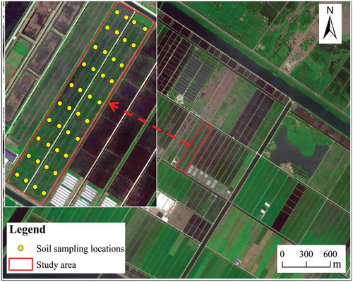
The terrain of Cixi City, Zhejiang Province, is higher in the south and lower in the north, with a three-level terrace of hills, plains, and mudflats unfolding towards Hangzhou Bay. It is located at the southern edge of the northern subtropical zone, which has a monsoon climate with an annual average temperature of 16°C and total precipitation of 1,272.8 mm. The study area is located in the National Modern Agricultural Industrial Park in the northern part of Cixi City, which is a part of the coastal historical reclamation area (surface area, approximately 6.5 ha). The soil type is paddy soil, which is neutral to slightly alkaline and contains soluble salts, and the crop rotation system primarily comprises soybean – wheat rotation. The distribution of the sampling points is shown in Figure 2.

Figure 2. RS image of the study area and spatial distribution of the sampling points.

2.3. Research data

2.3.1. Soil sampling and determination of organic matter

The soil samples were collected on 18 January 2022, when the study area was characterized by freshly tilled bare soil. The sampling points were evenly distributed according to a grid, and sheets of A4 paper were placed at the centre of the sampling points as markers. Forty soil samples were collected from 0–20 cm of the ploughed soil layer using the plum-shaped method of laying out sampling points within 1 m of the marking points, and the coordinate information of the marking points was recorded. The samples were air-dried, ground, and sieved, and the organic matter content was determined using oxidative titration with potassium dichromate.

2.3.2. UAV hyperspectral data acquisition

The Cubert S185 Airborne Imaging Spectrometer (Cubert GmbH, Ulm, Germany), a frame-type imaging spectrometer, combines the accuracy of hyperspectral data and the high speed of snapshot imaging; it can obtain high-spectral-resolution (4 nm) images in the 450–950 nm range in the entire field of view within 0.001 s. Compared with the traditional push-scan imaging spectrometer, this spectrometer is smaller, lighter, and more easily compatible with the UAV platform. It is suitable for use in the rapid monitoring of field-scale SOM. However, its prediction accuracy must be tested and verified.

Images were captured on 18 January 2022 during a flight time of 11:00–12:00 in clear and windless conditions. Before the flight, a DJI M300 UAV (DJI, Shenzhen, China) with a Cubert S185 airborne imaging spectrometer was used, and whiteboard and dark current corrections were performed. The spectral coverage consisted of 125 bands from 450 to 950 nm with a spectral resolution of 4 nm. The UAV flight altitude was 120 m, corresponding to a 3.12 cm image spatial resolution, and the course overlap rate and lateral overlap rates were both 80%. The obtained images underwent preprocessing, including the following steps: (1) checking the image quality and removing the UAV takeoff and landing images; (2) image stitching to generate orthophoto images; (3) geometric image correction; (4) the addition of band information.

2.3.3. Extraction of soil spectral data

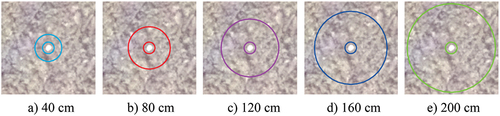
A region of interest (ROI) with an inner radius of 15 cm and an outer radius of 20–200 cm (at 20 cm intervals) was established to extract the soil spectral data, with the centre of the marker as the centre of the circle (Figure 3). An SVM model was established and cross-validated using the leave-one-out method to determine the optimal extraction range for the spectral modelling data.

Figure 3. Example of circular ROI with different outer radii.

2.3.4. Preprocessing of spectral data

The noise bands at both ends of the spectra were removed, 105 bands from within the range of 490–906 nm were retained, and the raw spectra (R) were the Savitzky – Golay (SG)-smoothed spectral curves. The R values were subjected to the standard normal variable (SNV), multiple scattering correction (MSC), and first derivative reflectance (FDR). The SNV is calculated by subtracting the mean value of the spectrum from the original spectrum and dividing it by the standard deviation of the spectrum, which can reduce the effect of uneven soil particle size and particle surface scattering (Rinnan, Berg, and Engelsen 2009). MSC can effectively eliminate the scattering effects caused by the uneven distribution of soil particles and particle size and improve the spectral information related to the SOM content in the spectral data (Isaksson and Næs 1988). First, the average value of all the spectral data was obtained, and then the spectra of each sample were linearly regressed with the average spectrum. The linear shift was subtracted from each sample spectrum and calculated by dividing it by the tilt offset. The spectral first-order differential transform amplifies small changes in the slope of the spectral curve and reduces the interference from the baseline translation, atmospheric scattering, and noise.

2.4. Construction of soil spectral indices

The main spectral indices (SI) used in this study are as follows: the difference index (DI), the ratio index (RI), and the normalized index (NDI). The calculation formulae are as follows:

(1) $\mathrm{DI}={\mathrm{R}}_{\mathrm{i}}-{\mathrm{R}}_{\mathrm{j}}$(1)

(2) $\mathrm{RI}={\mathrm{R}}_{\mathrm{i}}/{\mathrm{R}}_{\mathrm{j}}$(2)

(3) $\mathrm{NDI}=\left({\mathrm{R}}_{\mathrm{i}}-{\mathrm{R}}_{\mathrm{j}}\right)\mathit{\hspace{0.17em}}/\mathit{\hspace{0.17em}}({\mathrm{R}}_{\mathrm{i}}+{\mathrm{R}}_{\mathrm{j}})$(3)

where R_i and R_j represent the soil spectral reflectance in the i and j bands, respectively.

2.5. Modeling and accuracy evaluation

The accuracy of the model varies according to different sample set partitions (Lucà et al. 2017). The random sampling method was used to select 30 modelling samples and 10 prediction samples each time with a ratio of 3:1 between the modelling and prediction sets. By conducting 1000 random samplings, modelling, and predictions on the sample set, we analysed the results of 1000 calculations to reduce the impact of randomly dividing the sample set on the model results. In the table of modelling results, ‘Mean’ is the mean value of each accuracy index of the models constructed after 1000 random samplings, and ‘Best’ is the value of each accuracy index of the model with the highest prediction set R², which is regarded as the optimal model. The common linear model, PLSR, and the nonlinear model, SVM, are among the utilized modelling methods. For SVM, we used the Gaussian kernel function.

Independent validation was used to evaluate the prediction accuracy, and the coefficient of determination (R²), the root mean squared error (RMSE), and the ratio of performance to interquartile distance (RPIQ) were the indices selected to evaluate the model’s accuracy. The closer R² (modelling set R_c², prediction set R_p²) is to 1, the higher the model’s relevance and stability; the closer the RMSE (modelling set RMSE_c, prediction set RMSE_p) is to 0, and the closer the two are to each other, and the higher the predictive ability and stability of the model. The values of the prediction set samples were arranged from smallest to largest: the value at 1/4 of the arrangement was Q₁, the value at 3/4 was Q₃, and the interquartile spacing was the difference between Q₃ and Q₁. Bellon-Maurel et al. (2010) found that soil physicochemical data typically have a non-normal distribution and that the RPIQ is more objective than an evaluation based on the relative percent deviation (RPD). It is commonly assumed that, the larger the RPIQ, the better the predictive ability of the model; if RPIQ < 1.4, the model does not have any predictive ability; if 1.7 ≤ RPIQ < 2.0, the model has good predictive ability; if 2.0 ≤ RPIQ < 2.5, the model has very good predictive ability; and, if RPIQ ≥ 2.5, the model is excellent (Nawar and Mouazen 2017).

The pixel value for SOM was predicted according to the model. Then, the accuracy of the mapping results was evaluated by comparing the range, mean, standard deviation, coefficient of variation, kurtosis, and skewness of the SOM map with those of the sample set.

2.6. Data processing and mapping

First, the cross-validation results of the SVM models established using the spectral data extracted from different ranges of ROIs and measured SOM were compared to determine the optimal modelling spectral data for the study area. Then, based on the raw and transformed spectra, the correlation distribution of SOM with different spectra was analysed, and a SOM prediction model was established based on the full band. Next, the DI, RI, NDI, and their correlation coefficients with SOM were calculated, and the filtered spectral indices were used to establish the SOM prediction model and evaluate its accuracy. Finally, the optimal models based on the full band and spectral indices were applied to the hyperspectral images to realize the spatial distribution mapping of the SOM in the study area (Figure 1).

Data exporting was mainly performed using Cubert pilot software, and Agisoft PhotoScan software was used for the stitching process. Spectral transformation, correlation analysis, spectral index calculations, correlation coefficient isopotential plots, modelling, and SOM mapping were performed using MATLAB R2017b (The MathWorks Inc., Natick, MA, USA). Statistical analyses and data plotting were performed using Origin 2018 (OriginLab Corporation, Northampton, MA, USA).

3. Results

3.1. SOM content statistics

The standard deviation, coefficient of variation, kurtosis, and skewness were used to characterize the SOM content in the study area (Table 1). The SOM content in the study area was low (mean 14.29 g·kg⁻¹) with low spatial variability (minimum 7.82 g·kg⁻¹, maximum 24.4 g·kg⁻¹ and coefficient of variation 25.78%). The kurtosis of the SOM content was close to 3 (K = 2.78), indicating that the data were normally distributed. The skewness of the SOM content was greater than 0 (S = 0.35), with a right-skewed distribution, and the mean of the data was greater than the median and plurality, indicating that there were points in the sample with a very high SOM content.

Table 1. Statistical characteristics of SOM.

Number of samples	Minimum (g·kg^−1)	Maximum (g·kg^−1)	Average (g·kg^−1)	Standard deviation (g·kg^−1)	Coefficient of variation (%)	Kurtosis (K)	Skewness (S)
40	7.82	24.4	14.29	3.68	25.78	2.78	0.35

3.2. Optimal radius for extracting the spectral data

When the outer radius of the annular ROI used to extract the average spectra increased from 20 cm to 80 cm, the R² and RPIQ gradually increased, and the RMSE gradually decreased. When the outer radius of the annular ROI gradually increased from 80 cm, the R² and RPIQ values showed a decreasing trend, and the RMSE showed an increasing trend (Figure 4). Therefore, the spectra extracted from the annular ROI with an outer radius of 80 cm were modelled with the highest R² and RPIQ and the lowest RMSE, which is the optimal spectral extraction range for the study area.

Figure 4. Cross-validation results of the spectral and SOM modeling for circular ROI extraction with different outer radii.

To further compare the sensitive bands of SOM of soil spectra extracted at different ranges, the correlation coefficients between soil spectra and SOM were calculated separately. The top 10 bands with the highest correlation between soil spectra extracted at different ranges and SOM were shown in Table 2, and it is found that most of the sensitive bands are concentrated at the NIR band.

Table 2. Sensitive bands of SOM of soil spectra extracted at different ranges.

Outer radius of circular ROI	Sensitive bands of SOM/nm
20cm	530、566、650、822、874、878、882、938、942、946
40cm	510、514、518、530、566、822、878、882、942、946
60cm	510、514、518、566、858、874、878、882、942、946
80cm	510、514、518、822、858、862、874、878、882、946
100cm	478、514、518、854、858、862、874、878、882、946
120cm	854、858、862、870、874、878、882、910、914、946
140cm	858、862、870、874、878、882、906、910、914、946
160cm	858、878、882、902、906、910、914、918、942、946
180cm	902、906、910、914、918、922、934、938、942、946
200cm	902、906、910、914、918、922、934、938、942、946

3.3. The correlation between SOM and soil spectra

3.3.1. SOM and full band

Figure 5 depicts the absolute value distribution of the correlation coefficients between the soil spectra and the SOM content. The absolute values of the correlation coefficients between the SOM content and the raw spectra were all greater than 0.41. The correlation was greater than that of the other bands in the range of 586–894 nm, with the absolute values of correlation coefficients above 0.48 and a maximum value of 0.51 (Figure 5(a)). After transforming the raw spectra, the absolute values of the maximum correlation coefficients of SOM with SNV spectra and MSC spectra were 0.36 and 0.32. The absolute value of the maximum correlation coefficient of the FDR spectra with SOM was 0.59. Compared with the raw spectra, the absolute values of the maximum correlation coefficients of the transformed SNV and MSC spectra were reduced; the lowest value was close to 0, and the overall correlation was lower than that of the original spectra (Figure 5(b,c)). The absolute value of the maximum correlation coefficient between the FDR spectra and SOM increased to 0.59 after the first-order differential transformation, but the lowest value was also close to 0 (Figure 5(d)).

Figure 5. Absolute value of the correlation coefficient between the soil spectrum and SOM.

3.3.2. SOM and spectral indices

The correlation coefficient equipotential plot between the SOM content and spectral indices in the study area (Figure 6) shows the distribution range of the bands constituting the spectral indices with a high correlation coefficient. Different values indicate the absolute values of the correlation coefficients of DI, RI, and NDI computed from the combination of the two bands with SOM. In the raw spectra, there was a wide range of band combinations of SOM with a high correlation with DI, with distributions at 590–680 nm, and the absolute values of the correlation coefficients were above 0.6 at 630–650 nm (Figure 6(a)). The range of band combinations with strong correlations with RI and NDI was consistent and narrow, and the three largest correlation coefficients had the same values and band combinations (Figure 6(b,c)). In the SNV spectra, the band combinations with strong correlations between the SOM content and DI were mainly distributed at 630–690 nm, and the absolute values of the correlation coefficients were above 0.5 (Figure 6(d)). There were fewer band combinations with strong correlations with RI and NDI, and the correlation coefficients were lower (Figure 6(e,f)). The correlation distributions of DI, RI, NDI, and SOM in the MSC spectra were consistent with those in the SNV spectra (Figure 6(d,g-i)). The band combinations with stronger DI correlations between the SOM and FDR spectra were distributed across the entire spectral range (Figure 6j), as were the distributions of the band combinations with strong correlations with RI and NDI, but the band combinations with the highest correlation coefficients were slightly different (Figure 6(k,m)).

Figure 6. Correlation coefficient between SOM and spectral indices.

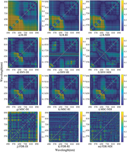
The absolute values of the correlation coefficients between the reflectance and SOM content of the raw spectra at 626 nm, 630 nm, 646 nm, and 650 nm ranged from 0.48–0.50 (Figure 5), and the correlations with the SOM content were significantly higher after calculating DI, RI, and NDI, with absolute correlation coefficients of more than 0.6. The SNV spectra and MSC spectra at 626 nm, 630 nm, 682 nm, and 686 nm showed significantly stronger correlations with SOM content after calculating the DI, RI, and NDI; and the FDR spectra at 530 nm, 554 nm, 582 nm, 618 nm, 646 nm, and 658 nm also showed significantly stronger correlations with SOM content after calculating the spectral indices.

3.4. SOM modeling

3.4.1. SOM modeling based on the full band

Four spectral datasets were used to establish the PLSR and SVM models for the SOM content in the study area, and the results are shown in Tables 3 and 4. The FDR spectra are slightly better in the results of PLSR modelling with 1000 random samplings, the R² values of the optimal model modelling set and prediction set are 0.55 and 0.44, respectively, and the R² values of the modelling set and prediction set of the remaining three spectral optimal models are less than 0.3, with poorer predictive ability. As shown in Table 4, among the 1000-times SVM modelling results, the optimal model’s modelling and prediction sets of the raw spectra can reach 0.8 and 0.72 respectively, with a prediction set RMSE of 1.38 g·kg⁻¹ and an RPIQ of 2.67; this allows the model to make more accurate predictions about the SOM content, making it the best model among the four spectra. For the remaining three spectra, the optimal model has a modelling set R² value of about 0.7, a prediction set R² value of about 0.55, and an RMSE of about 2 g·kg⁻¹. The model’s accuracy was slightly lower than that of the raw spectra, but it also had a certain level of predictive ability across 1000 modelling runs.

Table 3. Full-band PLSR regression modelling results.

Spectra		Rc^2	RMSEc	Rp^2	RMSEp	RPIQ
R	Best	0.25	3.43	0.25	2.11	1.51
	Mean	0.26	3.05	0.13	3.42	1.67
SNV	Best	0.25	3.39	0.24	2.04	1.42
	Mean	0.17	3.22	0.16	3.67	1.67
MSC	Best	0.29	3.27	0.26	2.40	2.09
	Mean	0.15	3.27	0.07	3.58	1.67
FDR	Best	0.55	2.52	0.44	2.46	2.80
	Mean	0.43	2.67	0.17	3.32	1.74

Table 4. Full-band SVM modelling results.

Spectra		Rc^2	RMSEc	Rp^2	RMSEp	RPIQ
R	Best	0.80	1.57	0.72	1.38	2.67
	Mean	0.73	1.86	0.18	3.22	1.85
SNV	Best	0.69	2.10	0.58	1.99	2.92
	Mean	0.77	1.68	0.14	3.49	1.70
MSC	Best	0.71	2.07	0.50	2.05	2.88
	Mean	0.77	1.67	0.14	3.56	1.70
FDR	Best	0.74	1.84	0.55	2.52	2.38
	Mean	0.80	1.60	0.20	3.13	1.86

3.4.2. SOM modeling based on spectral indices

In each of the four spectra, the top 10 indices with the highest correlation between each spectral index and SOM were selected to build an SVM model to predict the SOM content in the study area, and the results are shown in Table 5. Among the four spectra, in general, the modelling results of the FDR spectra were better than those of the other three spectra, and the optimal models of the three spectral indices based on the FDR spectra had R² values for the modelling set and prediction set above 0.7, an RMSE value of less than 2 g·kg⁻¹, and an RPIQ greater than 3. In the case of the NDI model based on the FDR spectra, the optimal model exhibited a modelling set R_c² value of up to 0.83, a prediction set R_p² value of up to 0.77, a prediction set RMSE_p of only 1.3 g·kg⁻¹, and an RPIQ that reached 4.76. Compared to all of the models developed using spectral indices, this model is excellent, exhibiting the highest accuracy. This model is also more generalizable, as its modelling set and prediction set R² values are relatively close to each other. The mean RPIQ values of the nine spectral index models developed for the final three spectra are between 1.68 and 1.89, showing better predictive abilities and varying degrees of improvement over the full-band modelling results (Table 4). The NDI model based on the FDR spectra has a mean RPIQ value of 2.21 and exhibits excellent predictive ability. By calculating the spectral indices, the input variables of SOM modelling were reduced, the modelling efficiency was improved, and the accuracy of the modelling prediction was improved to some extent.

Table 5. SVM modelling results of spectral indices.

Spectra	Spectral indices		Rc^2	RMSEc	Rp^2	RMSEp	RPIQ
R	DI	Best	0.58	2.51	0.56	1.85	1.57
		Mean	0.59	2.27	0.22	3.22	1.86
	RI	Best	0.62	2.27	0.57	2.25	2.89
		Mean	0.66	2.09	0.16	3.26	1.85
	NDI	Best	0.63	2.36	0.59	1.87	3.10
		Mean	0.66	2.11	0.17	3.22	1.89
SNV	DI	Best	0.61	2.41	0.42	2.14	2.58
		Mean	0.57	2.31	0.14	3.47	1.72
	RI	Best	0.51	2.66	0.45	2.29	2.62
		Mean	0.53	2.48	0.13	3.29	1.86
	NDI	Best	0.58	2.41	0.53	2.32	2.15
		Mean	0.63	2.21	0.17	3.19	1.85
MSC	DI	Best	0.60	2.49	0.51	1.76	2.78
		Mean	0.58	2.28	0.13	3.53	1.68
	RI	Best	0.50	2.68	0.44	2.22	2.03
		Mean	0.52	2.47	0.12	3.42	1.72
	NDI	Best	0.47	2.87	0.45	1.75	2.29
		Mean	0.51	2.50	0.13	3.38	1.78
FDR	DI	Best	0.71	1.96	0.70	1.97	3.50
		Mean	0.72	1.90	0.30	2.94	1.96
	RI	Best	0.79	1.80	0.76	1.21	3.57
		Mean	0.80	1.61	0.30	2.91	2.01
	NDI	Best	0.83	1.58	0.77	1.30	4.76
		Mean	0.81	1.56	0.41	2.61	2.21

3.5. SOM mapping based on optimal models

Using the modelling results shown in Tables 3 and 4, the optimal SOM prediction model was selected, and a scatter plot was plotted (Figure 7). Different degrees of deviation were observed between the predicted and measured values of the models. The R-SVM model was more likely to underestimate the SOM content than the FDR-NDI-SVM model when the SOM content was higher than 14 g.kg⁻¹. Overall, the SVM model based on the FDR spectra combined with NDI was the best of all the models, with the predicted and measured values more evenly distributed around the 1:1 line.

Figure 7. Scatter plot of the SOM content predicted by the optimal model.

We applied the two optimal models to the hyperspectral images, inverted the SOM content of the study area on a pixel-by-pixel basis, and generated a SOM spatial distribution map (Figure 8). Both models predicted a distribution of SOM that was high in the south and low in the north, which was similar to the distribution of the measured values. The R-SVM model better reflected this feature, while the FDR-NDI-SVM model reduced the phenomena of the overestimation of low values and the underestimation of high values. The mapping results of both models agreed well with the measured SOM values.

Figure 8. Spatial distribution of the SOM content based on optimal model inversion.

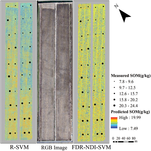
Table 6 shows the statistics of the values of all pixels in the mapping results and measured values of soil sampling points. The predicted SOM content values ranged from 9.25 to 18.36 g kg⁻¹ and 7.49 to 19.99 g·kg⁻¹. The values of the distribution map predicted by the FDR-NDI-SVM model are closer to the measured values in terms of range, mean value, and standard deviation.

Table 6. Statistical characteristics of soil organic matter content based on optimal model inversion.

Predicted Model/ Measured Value	Minimum (g·kg^−1)	Maximum (g·kg^−1)	Average (g·kg^−1)	Standard Deviation (g·kg^−1)
R-SVM	9.25	18.36	13.77	1.57
FDR-NDI-SVM	7.49	19.99	14.17	1.58
Measured value	7.82	24.4	14.29	3.68

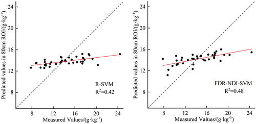
To further quantitatively analyse the mapping accuracy, the predicted values of the pixels within 80 cm of sampling marker were extracted from the SOM spatial distribution map and averaged, which were regarded as the mapping prediction of this sampling point, and plotted on a scatter plot with the measured values (Figure 9). The fitted R² of the mapping results of the R-SVM model was 0.42, and that of the FDR-NDI-SVM model was improved to 0.48, which indicated that the FDR-NDI-SVM model was not only superior to the R-SVM model in terms of modelling accuracy, but also outperformed than the R-SVM model in terms of mapping accuracy.

Figure 9. Scatter plot of predicted mean values within 80 cm of sampling markers versus measured values.

4. Discussion

4.1. Extraction range for the optimal spectral data

Some studies have used spectral imaging data to predict soil properties (Aldana-Jague et al. 2016; Franceschini et al. 2015), but few have discussed the optimal spectral extraction range. In this study, an annular ROI with an outer radius of 20–200 cm was established at 20 cm intervals centred around the soil sampling marker point to extract the average spectra and model of the SOM. The results showed that the annular ROI with an outer radius of 80 cm had the highest modelling accuracy and was the optimal extraction range of the soil spectra in the study area, which was related to the sampling method used in this study. In this study, the soil samples were collected within 1 m of the marker point using the plum-shaped method, and the 80 cm annular ROI covered the majority of the pixels in the soil extraction location, with a high correlation between the extracted spectral information and the SOM. The annular ROI larger than 80 cm mixed in more spectral information unrelated to the soil extraction location, resulting in a gradual decrease in modelling accuracy. An annular ROI smaller than 80 cm could not cover all the soil extraction locations, and, as the radius of the ROI decreased, fewer soil extraction locations were covered, and the accuracy of the model was lower. Therefore, in subsequent imaging spectral mapping studies, it is important to consider the effect of the soil sampling method on the quality of spectral extraction; the extraction range of the average spectral data should cover as many soil extraction pixels as possible and minimize the mixing of non-soil extraction pixels.

4.2. Correlation between soil spectra and SOM

The sensitive bands for the inversion of the SOM content in the study area were mainly located at 630–710 nm, 750–790 nm, and 810–890 nm, which is consistent with the results of numerous previous studies (Lu et al. 2007; Peng et al. 2013; M. Wang et al. 2011; Zhang et al. 2009). The predictions based on the full-band SNV and MSC spectra were roughly the same because of the similar distribution of correlations between SNV and MSC spectra and SOM (Tables 1 and 2). The modelling results of the 1000 random samplings for the raw spectra were almost identical, which is due to the same band combinations of RI and NDI being selected; the modelling results in the SNV and MSC spectra were also nearly identical due to the distribution of correlations of DI, RI, and NDI with SOM content being roughly the same in the SNV and MSC spectra (Table 3). This indicates that the correlation between spectra and SOM can serve as an important basis for the selection of bands.

4.3. Spectral processing and indices

The use of SG and first-order differentiation algorithms can effectively weaken the sensitive bands of moisture and diminish the overlapping interference of soil moisture on the bands of soil fertility attributes (Hu et al. 2021). In this study, the accuracy of the spectral index model based on the FDR spectra was generally higher than that based on the other spectra, which is consistent with previous findings. According to the modelling results, the SVM model achieved the highest prediction accuracy based on the NDI of the FDR spectra, with the highest model prediction set R² value of 0.77 and an RPIQ of 4.76. Y. Guo et al. (2013) showed that the prediction of SOM content can be improved by constructing spectral indices and that RI and NDI are the most effective of these indices, a conclusion similar to the findings of this study. By creating spectral indices, the correlation coefficients between reflectance and SOM in the different bands of the four spectra were improved to varying degrees, the efficiency and accuracy of later model prediction and SOM mapping was also improved to some extent.

Comparing the range of measured and predicted SOM values, we found that, in the mapping results of the FDR-NDI-SVM model, the underestimation of high values and overestimation of low values were reduced; this indicates that the model built using spectral indices reduced redundant band information in the hyperspectral data and improved the accuracy of the model’s predictions. Therefore, subsequent studies based on this foundation should consider adding a characteristic band-filtering algorithm to select spectral feature bands in an attempt to improve prediction accuracy.

4.4. SOM modelling and Mapping

Regarding SOM mapping, some scholars have used spatial interpolation in geostatistics (Y. Guo et al. 2013, 2016), which can obtain the approximate distribution of SOM over a large area. However, the predicted values become more inaccurate as one moves away from the measured SOM value. Some scholars have also conducted SOM mapping using satellite data (H. Liu et al. 2020) and aerial hyperspectral data (D. Wang et al. 2018), but there are issues related to the difficulty of data acquisition and large spatial resolutions, which cannot meet the demands of precision agriculture. In this study, SOM mapping was performed based on UAV imaging spectroscopy with a centimetre-level spatial resolution, and the predicted maps of both models showed the same spatial variability trend as the measured values (Figure 8), indicating that this technology can be applied to the rapid real-time acquisition of field-scale SOM spatial distribution information.

In previous studies of the indoor spectral prediction of SOM, the PLSR method generally achieved high accuracy. However, in this study, PLSR could not accurately predict SOM. Previous studies have pointed out that SOM content and soil spectra often exhibit a nonlinear relationship (Yan, Yao, and Zhang 2019) which cannot be adequately reflected by the linear PLSR model (J. K. M. Biney et al. 2023). Furthermore, the spectral imaging data for bare farmland soil were collected directly in the field, without the soil first being processed with air-drying, grinding, or sieving. This increased the influence of soil moisture, surface roughness, and many other environmental factors on the soil spectra and further enhanced the nonlinear relationship between the soil spectra and SOM. Compared to the linear model, the SVM can more effectively deal with nonlinear problems in hyperspectral information, resulting in higher prediction accuracy. The nonlinear SVM model used in this study achieved an overall higher prediction accuracy than the linear PLSR model.

4.5. The number of samples

The number of soil samples collected in this study was 40; this number may seem small, but the density of samples is more important than the number. The density of samples in this study was about 6.2 samples per hectare, and previous studies (J. K. M. Biney et al. 2023; L. Guo et al. 2020; Heil, Jörges, and Stumpe 2022; Yang et al. 2021) with densities of samples ranging from 6.07 to 10.7 samples per hectare have achieved better results. The sample density of this study is within a reasonable range.

Furthermore, the airborne imaging spectrometer used in this study has a band range of 450–950 nm; as sensors develop and become more popular, an increase in the number of data in the 1000–2500 nm range will further improve SOM prediction accuracy. Compared with indoor spectral measurements, the acquisition of imaging spectral data via the UAV platform is affected by environmental factors such as soil moisture, and more research is needed to determine how to eliminate or mitigate these environmental impact factors.

5. Conclusion

In this study, we captured imaging spectral data from a coastal reclamation area using a Cubert S185 airborne imaging spectrometer mounted on a UAV platform. The average spectral data were first extracted via circular regions of interest (ROIs) of different radii. Then, the optimal models for SOM mapping were investigated in terms of spectral indices and modelling algorithms (i.e. PLSR and SVM). The results showed the following:

1. The optimal extraction radius of spectral data is 80 cm, which was related to the sampling method of soil;

2. The accuracy of the nonlinear SVM model is much higher than that of the linear PLSR model due to the influence of soil moisture and surface roughness in the field environment;

3. The prediction model based on spectral indices (with the predicted R² and RMSE values of 0.42-0.77 and 1.30-2.32 g·kg⁻¹) is better than the full band model. Moreover, the calculation of the spectral indices improved the correlation between spectra and SOM. The accuracy of prediction and efficiency of SOM mapping was also improved.

The imaging spectrometer, in conjunction with the UAV, can accurately map SOM content, enabling us to rapidly monitor SOM changes, thus providing data support for precision agriculture and climate change studies.

Acknowledgements

The authors of this study would like to express their thanks to the key project of the National Natural Science Foundation (grant number: 42130405), the National Natural Science Foundation of China (grant numbers: 42371060 and 42301478) project, and the Science and Technology Project of the Department of Natural Resources of Zhejiang Province (grant number: 2020-33) for their support.

Disclosure statement

No potential conflict of interest was reported by the author(s).

Additional information

Funding

This work was supported by the Key project of the National Natural Science Foundation [42130405]; National Natural Science Foundation of China [42371060]; National Natural Science Foundation of China [42301478]; Science and Technology Project of Department of Natural Resources of Zhejiang Province [2020-33].

References

- Aldana-Jague, E., G. Heckrath, A. Macdonald, B. van Wesemael, and K. Van Oost. 2016. “UAS-Based Soil Carbon Mapping Using VIS-NIR (480–1000nm) Multi-Spectral Imaging: Potential and Limitations.” Geoderma 275:55–66. https://doi.org/10.1016/j.geoderma.2016.04.012.
- Angelopoulou, T., N. Tziolas, A. Balafoutis, G. Zalidis, and D. Bochtis. 2019. “Remote Sensing Techniques for Soil Organic Carbon Estimation: A Review.” Remote Sensing 11 (6): 676. https://doi.org/10.3390/rs11060676.
- Bellon-Maurel, V., E. Fernandez-Ahumada, B. Palagos, J.-M. Roger, and A. McBratney. 2010. “Critical Review of Chemometric Indicators Commonly Used for Assessing the Quality of the Prediction of Soil Attributes by NIR Spectroscopy.” Trends in Analytical Chemistry 29 (9): 1073–1081. https://doi.org/10.1016/j.trac.2010.05.006.
- Biney, J. K. M., J. Houška, J. Volánek, D. K. Abebrese, and J. Cervenka. 2023. “Examining the Influence of Bare Soil UAV Imagery Combined with Auxiliary Datasets to Estimate and Map Soil Organic Carbon Distribution in an Erosion-Prone Agricultural Field.” Science of the Total Environment 870:161973. https://doi.org/10.1016/j.scitotenv.2023.161973.
- Biney, J. K., M. Saberioon, L. Borůvka, J. Houška, R. Vašát, P. Chapman Agyeman, J. A. Coblinski, and A. Klement. 2021. “Exploring the Suitability of UAS-Based Multispectral Images for Estimating Soil Organic Carbon: Comparison with Proximal Soil Sensing and Spaceborne Imagery.” Remote Sensing 13 (2): 308. https://doi.org/10.3390/rs13020308.
- Cao, J., and H. Yang. 2023. “A Dynamic Normalized Difference Index for Estimating Soil Organic Matter Concentration Using Visible and Near-Infrared Spectroscopy.” Ecological Indicators 147:110037. https://doi.org/10.1016/j.ecolind.2023.110037.
- Chen, H., G. Yang, X. Han, X. Liu, F. Liu, and N. Wang. 2021. “Hyperspectral Inversion of Soil Organic Matter Content Based on Continuous Wavelet Transform.” Journal of Agricultural Science and Technology 23 (5): 132–142. https://doi.org/10.13304/j.nykjdb.2020.0742.
- Franceschini, M. H. D., J. A. M. Demattê, F. da Silva Terra, L. E. Vicente, H. Bartholomeus, and C. R. de Souza Filho. 2015. “Prediction of Soil Properties Using Imaging Spectroscopy: Considering Fractional Vegetation Cover to Improve Accuracy.” International Journal of Applied Earth Observation and Geoinformation 38:358–370. https://doi.org/10.1016/j.jag.2015.01.019.
- Guo, Y., Y. Cheng, L. Wang, T. Liu, S. Chen, and G. Zheng. 2016. “Prediction and Mapping of Soil Organic Matter Content Using Hyperspectral and GF-1 Multi-Spectra.” Chinese Journal of Soil Science 47 (3): 537–542. https://doi.org/10.19336/j.cnki.trtb.2016.03.05.
- Guo, L., P. Fu, T. Z. Shi, Y. Chen, H. Zhang, R. Meng, and S. Wang. 2020. “Mapping Field-Scale Soil Organic Carbon with Unmanned Aircraft System-Acquired Time Series Multispectral Images.” Soil and Tillage Research 196:104477. https://doi.org/10.1016/j.still.2019.104477.
- Guo, Y., W. Ji, H. Wu, and Z. Shi. 2013. “Estimation and Mapping of Soil Organic Matter Based on Vis-NIR Reflectance Spectroscopy.” Spectroscopy and Spectral Analysis 33 (4): 1135–1140. https://doi.org/10.3964/j.issn.1000-059304-1135-06.
- Heil, J., C. Jörges, and B. Stumpe. 2022. “Fine-Scale Mapping of Soil Organic Matter in Agricultural Soils Using UAVs and Machine Learning.” Remote Sensing 14 (14): 3349. https://doi.org/10.3390/rs14143349.
- Hu, Y., X. Gao, Z. Shen, Y. Xiao. 2021. “Estimating Fertility Index by Using Field-Measured Vis-NIR Spectroscopy in the Huanghui River Basin.” Chinese Journal of Soil Science 52 (3): 575–584. https://doi.org/10.19336/j.cnki.trtb.2020080701.
- Isaksson, T., and T. Næs. 1988. “The Effect of Multiplicative Scatter Correction (MSC) and Linearity Improvement in NIR Spectroscopy.” Applied Spectroscopy 1988 (7): 1273–1284. https://doi.org/10.1366/0003702884429869.
- Jin, X., K. Song, J. Du, H. Liu, and Z. Wen. 2017. “Comparison of Different Satellite Bands and Vegetation Indices for Estimation of Soil Organic Matter Based on Simulated Spectral Configuration.” Agricultural and Forest Meteorology 244-245:57–71. https://doi.org/10.1016/j.agrformet.2017.05.018.
- Liu, H., Y. Bao, X. Meng, Y. Cui, A. Zhang, Y. Liu, and D. Wang. 2020. “Inversion of Soil Organic Matter Based on GF-5 Images Under Different Noise Reduction Methods.” Transactions of the Chinese Society of Agricultural Engineering (Transactions of the CSAE) 36 (12): 90–98. https://doi.org/10.11975/j.issn.1002-6819.2020.12.011.
- Liu, L., R. Shen, and G. Ding. 2011. “Studies on the Estimation of Soil Organic Matter Content Based on Hyper-Spectrum.” Spectroscopy and Spectral Analysis 31 (3): 762–766. https://doi.org/10.3964/j.issn.1000-0593(2011)03-0762-05.
- Lu, Y., Y. Bai, L. Wang, and H. Wang. 2007. “Prediction and Validation of Soil Organic Matter Content Based on Hyperspectrum.” Scientia Agricultura sinica 9:1989–1995. https://doi.org/10.3864/j.issn.0578-1752.au-2007-00071.
- Lucà, F., M. Conforti, A. Castrignanò, G. Matteucci, and G. Buttafuoco. 2017. “Effect of Calibration Set Size on Prediction at Local Scale of Soil Carbon by Vis-NIR Spectroscopy.” Geoderma 288:175–183. https://doi.org/10.1016/j.geoderma.2016.11.015.
- Nawar, S., H. Buddenbaum, J. Hill, J. Kozak, and A. M. Mouazen. 2016. “Estimating the Soil Clay Content and Organic Matter by Means of Different Calibration Methods of Vis-NIR Diffuse Reflectance Spectroscopy.” Soil and Tillage Research 155:510–522. https://doi.org/10.1016/j.still.2015.07.021.
- Nawar, S., and A. M. Mouazen. 2017. “Predictive Performance of Mobile Vis-Near Infrared Spectroscopy for Key Soil Properties at Different Geographical Scales by Using Spiking and Data Mining Techniques.” Catena 151:118–129. https://doi.org/10.1016/j.catena.2016.12.014.
- Pärnpuu, S., A. Astover, T. Tõnutare, P. Penu, and K. Kauer. 2022. “Soil Organic Matter Qualification with FTIR Spectroscopy Under Different Soil Types in Estonia.” Geoderma Regional 28:e00483. https://doi.org/10.1016/j.geodrs.2022.e00483.
- Peng, J., Q. Zhou, Y. Zhang, and H. Xiang. 2013. “Effect of Soil Organic Matter on Spectral Characteristics of Soil.” Acta Pedologica Sinica 50 (3): 517–524. https://doi.org/10.11766/trxb201207080277.
- Perz, R., and K. Wronowski. 2018. “UAV Application for Precision Agriculture.” Aircraft Engineering and Aerospace Technology 91 (2): 257–263. https://doi.org/10.1108/AEAT-01-2018-0056.
- Rinnan, Å., F. V. D. Berg, and S. B. Engelsen. 2009. “Review of the Most Common Pre-Processing Techniques for Near-Infrared Spectra.” TrAC Trends in Analytical Chemistry 28 (10): 1201–1222. https://doi.org/10.1016/j.trac.2009.07.007.
- Rossel, R. A. V., and T. Behrens. 2010. “Using Data Mining to Model and Interpret Soil Diffuse Reflectance Spectra.” Geoderma 158 (1–2): 46–54. https://doi.org/10.1016/j.geoderma.2009.12.025.
- Shanmugapriya, P., S. Rathika, T. Ramesh, and P. Janaki. 2019. “Applications of Remote Sensing in Agriculture - a Review.” International Journal of Current Microbiology and Applied Sciences 8 (1): 2270–2283. https://doi.org/10.20546/ijcmas.2019.801.238.
- Sun, G., W. Huang, P. Chen, S. Gao, and X. Wang. 2018. “Advances in UAV-Based Multispectral Remote Sensing Applications.” Transactions of the Chinese Society for Agricultural Machinery 49 (3): 1–17. https://doi.org/10.6041/j.issn.1000-1298.2018.03.001.
- Tang, H., X. Meng, X. Su, T. Ma, H. Liu, Y. Bao, M. Zhang, X. Zhang, and H. Huo. 2021. “Hyperspectral Prediction on Soil Organic Matter of Different Types Using CARS Algorithm.” Transactions of the Chinese Society of Agricultural Engineering (Transactions of the CSAE) 37 (2): 105–113. https://doi.org/10.11975/j.issn.1002-6819.2021.2.013.
- Wang, D., K. Qin, Z. Li, Y. Zhao, W. Chen, and Y. Gan. 2018. “Retrieval of Organic Matter Content in Black Soil Based on Airborne Hyperspectral Remote Sensing Data: Taking Jiansanjiang District in Heilongjiang Province As an Example.” Earth Science 43 (6): 2184–2194. https://doi.org/10.3799/dqkx.2018.612.
- Wang, M., X. Xie, R. Zhou, B. Wang, C. Wang, Y. Liu, J. Pan, R. Shen, and X. Pan. 2011. “Determination of Soil Organic Matter in Red Soils Using Vis-NIR Diffuse Reflectance Spectroscopy and Selection of Optimal Spectral Bands.” Acta Pedologica Sinica 48 (5): 1083–1089. https://doi.org/10.11766/trxb201006110237.
- Xiao, D., J. Huang, J. Li, Y. Fu, Y. Mao, Z. Li, and N. Bao. 2023. “Inversion Study of Soil Organic Matter Content Based on Reflectance Spectroscopy and the Improved Hybrid Extreme Learning Machine.” Infrared Physics & Technology 128:104488. https://doi.org/10.1016/j.infrared.2022.104488.
- Xu, S., M. Wang, and X. Shi. 2020. “Hyperspectral Imaging for High-Resolution Mapping of Soil Carbon Fractions in Intact Paddy Soil Profiles with Multivariate Techniques and Variable Selection.” Geoderma 370:114358. https://doi.org/10.1016/j.geoderma.2020.114358.
- Yang, X., N. Bao, E. Cao, and S. Liu. 2021. “Estimation and Mapping of Soil Nutrient in Farmland Based on UAV Imaging Spectrometry.” Geography and Geo-Information Science 37 (5): 38–45. https://doi.org/10.3969/j.issn.1672-0504.2021.05.006.
- Yan, X., Y. Yao, and X. Zhang. 2019. “The Progress and Prospect of Soil Organic Matter Mapping Based on Remote Sensing Technology.” China Agricultural Informatics 31 (3): 13–26. https://doi.org/10.12105/j.issn.1672-0423.20190302.
- Yu, L., Y. Hong, L. Geng, Y. Zhou, Q. Zhu, J. Cao, and Y. Nie. 2015. “Hyperspectral Estimation of Soil Organic Matter Content Based on Partial Least Squares Regression.” Transactions of the Chinese Society of Agricultural Engineering (Transactions of the CSAE) 31 (14): 103–109. https://doi.org/10.11975/j.issn.1002-6819.2015.14.015.
- Zhang, J., Y. Tian, Y. Zhu, X. Yao, and W. Cao. 2009. “Spectral Characteristics and Estimation of Organic Matter Contents of Different Soil Types.” Scientia Agricultura sinica 42 (9): 3154–3163. https://doi.org/10.3864/j.issn.0578-1752.2009.09.017.
- Zhao, M., Y. Xie, L. Lu, D. Li, and S. Wang. 2021. “Modeling for Soil Organic Matter Content Based on Hyperspectral Feature Indices.” Acta Pedologica Sinica 58 (1): 42–54. https://doi.org/10.11766/trxb202004200691.
- Zheng, G. H., D. Ryu, C. X. Jiao, C. Hong. 2016. “Estimation of Organic Matter Content in Coastal Soil Using Reflectance Spectroscopy.” Pedosphere 26 (1): 130–136. https://doi.org/10.1016/S1002-0160(15)60029-7.
- Zheng, G., A. Wang, C. Zhao, M. Xu, C. Jiao, and R. Zeng. 2023. “Evolution of Paddy Soil Fertility in a Millennium Chronosequence Based on Imaging Spectroscopy.” Geoderma 429:116258. https://doi.org/10.1016/j.geoderma.2022.116258.
- Zhou, W., L. Xie, Y. Han, L. Huang, H. Li, and Y. Meng. 2021. “Hyperspectral Inversion of Soil Organic Matter Content in the Three-Rivers Source Region.” Chinese Journal of Soil Science 52 (3): 564–574. https://doi.org/10.19336/j.cnki.trtb.2020051001.
- Zhou, J., Y. Xu, X. Gu, T. Chen, Q. Sun, S. Zhang, and Y. Pan. 2023. “High-Precision Mapping of Soil Organic Matter Based on UAV Imagery Using Machine Learning Algorithms.” Drones 7 (5): 290. https://doi.org/10.3390/drones7050290.