Prediction of mud loss in reservoir rock by geostatistical method

Abstract

In Iranian oil fields, Asmari Formation has great importance during the drilling operation because most of the oil reservoirs are located in this formation. One of the problems commonly encountered by petroleum engineers during drilling in the Asmari Formation is mud loss. The geostatistical methods can convert the qualitative experience to quantitative and provides the approach for better results.

There are different methods for the three-dimensional (3D) modelling of a reservoir. In this study, the distribution model of mud loss was designed for Asmari Formation using geostatistical methods and based on data of 389 wells drilled in an oil field in Southwest Iran.

1. Introduction

Asmari Formation has high capacity of storage (high porosity) and high ability of transmission fluid (high permeability) in this formation. This condition has led that many of oil reservoirs in the southwest of Iran are located in this formation.

Lost circulation is one of the most trouble-making and expensive problems in drilling the Asmari Formation in oil wells and the cost of lost materials, drilling equipment and time of drilling reaches millions of dollars per year. Lost circulation is defined as the loss of quantities of drilling fluid or cement slurry due to porosity of formation. The loss may vary from minor amounts to a complete loss of drilling fluid. Several oil companies have asked for a new solution to reduce or eliminate lost circulation trouble which can increase the cost of drilling from several hundred thousand to a million dollars per well. These unexpected costs are due to factors such as loss of time and drilling mud (Rueda 2000).

Types of lost circulation are determined based on the amount of loss, so the mud loss can be classified as (a) seeping, (b) partial, and (c) complete losses.

1.1. Seepage losses

Typically, losses up to approximately 10 bbl/hr are considered as seepage losses. Seepage losses are controlled simply by reducing or stopping the pump. By stopping the pump, the formation becomes sealed by the development of a filter cake. The pump rate can be gradually increased after the losses have stopped. If the loss is not stopped spontaneously and results in increasing economic costs, the LCM cells must be pumped into the wellbore to control it.

1.2. Partial losses

Losses from 10 bbl/hr up to 100 bbl/hr are often referred to as partial losses. The condition will usually need to be controlled. To control the loss, the pump must be turned off and the bit pulled up from the well. If the losses stop, drilling can be resumed, with reduced drilling fluid weight and/or pump rate, if these two actions are possible. Partial losses occur in gravels, small natural horizontal fractures, and barely opened induced vertical fractures.

1.3. Complete losses

Losses of more than 100 bbl/hr are considered as complete losses. Complete losses occur in sections of gravels, natural horizontal fractures, and partially opened induced vertical fractures. Severe complete losses occur in large opened natural horizontal fractures and wide opened induced vertical fractures (Mansuri 2002).

Mud losses can occur in any type of formation. Loss zones can be classified as (1) porous sand and gravels (2) vuggy formation (3) natural or intrinsic fractures (4) induced fractures.

3D geological models play an important role in petroleum engineering. There are different methods for 3D modelling, and mathematical or statistical information is used in each of these geological methods (Jennings et al. 2002). There are also several software tools for modelling various aspects of the reservoir.

Geostatistical methods are used to characterize reservoir heterogeneity on scales smaller than the distance between the wells (Dimitrakopoulos & Desbarats 1997). At present, the geostatistical method is a powerful tool for modelling. Generally, geostatistics is the study of the change of phenomena in terms of space or time. Essential components in geostatistics studies are:

1.	Evaluation of the data normal distribution (normalization analysis)
2.	Variogram analysis
3.	Kriging
4.	Stochastic simulation

In geostatistics studies variables are selected randomly. A random variable is a variable in which any value in its range has a certain probability to occur.

In geostatistics, the variables that have spatial structure are studied. So, in the first step, the spatial structure of the data should be determined. Therefore, based on the geostatistics viewpoint, each sample has a spatial relationship with the other samples around it up to a certain maximum distance. This maximum distance, which is called the effective radius, is very important, and in fact it indicates the distance in which statistical estimations can be used (Isaak & Serivaster 1989). Therefore, in geostatistics studies, the unknown data quantity in a specific coordinate can be estimated using the same quantity in the other known coordinates within the effective radius (Ortiz & Deutsch 2002).

2. Normalization analysis

The frequency distribution method is one of the simplest ways to analyse sample data. It summarizes the data in a more compact form than the original sample observations. To construct a frequency distribution, the range of the data is divided into intervals called class intervals. It is a common practice to use class sizes of equal width, but this is not necessary. The number of measurements falling within a particular class is called frequency (Webster & Oliver 2007).

There are several methods to assess normal data distribution. The two most common methods are considered below:

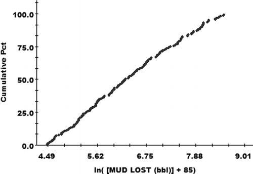
The first method is a graphical approach, so that the cumulative frequency curve of data is plotted according to high-level categories on a paper of which one of the axes is an arithmetic scale and the other axis a logarithmic scale. Since the cumulative frequency curve of a normal distribution in terms of high-level categories in these coordinates is a straight line, the closer the extension of the sum of points plotted on this paper to a straight line, the closer the data distribution to normal.

The second method for evaluating normal distribution of data is the qualitative method. For this purpose, it is sufficient to plot the histogram of data. If the histogram of data is near-normal with data skewness close to zero and data kurtosis close to three, then the data distribution is normal.

In case of non-normal distribution of data, there are various ways to transform them to a normal distribution, due to the more frequently used logarithmic method explained here. In this case, through the transformation of data under log transformation function, distribution of transformed data becomes symmetrical and close to normal distribution. Distribution of such data is called log normal distribution. Log normal distribution function is defined as follows:

in which α and β have been transformed to mean and standard deviation of functions, respectively, and can be calculated from the below equations:

Having α and β and the above distribution functions, mean and SD of data can be calculated as follows:

where ɛ is an infinitesimal positive number. LnX integral is not defined at the point X = 0. Thus, the e value is used to define the lower limit of integration. The confidence level in this case, as well as the normal distribution function, is calculated for the transformed data of which the distribution is normal, and then the following equation is used to calculate the true value of upper level (UL) and lower limit (LL):

The value of α _u and α _ul is calculated from the following equation:

3. Variogram analysis

Variogram analysis is an important part of geostatistical modelling. Indeed, variogram shows the mean square difference between the two values as a function of their increment (Cressie & Hawkins 1980). The value of variogram is calculated by the following equation:

In the above equation, γ(h) is called semivariogram and 2γ(h) is called variogram, and n_h is the number of pairs of points with the distance h from each other participating in the variogram. x_i is grade in point i and x _{i + h} is grade in a point with distance h from the point I. By calculating variogram for different h values, the γ(h) diagram in terms of h can be drawn, and the h value is called lag.

The experimental variograms usually begin from a non-zero value and increase up to a range called effective range (a), which eventually reaches the constant value called sill. The effective range is the range in which the data spatial structure is relevant, and outside the range, the data effects are independent from each other (Corstange et al. 2008).

Theoretically, the value of variogram for h = 0 should tend towards its minimum value of zero, but in practice, true variograms which are as a result of experience, do not usually follow this condition. The value of variogram for h = 0 is called Nugget effect. As h is increased, variogram begins from low values and tends towards a constant limit, so some variograms reach a relatively constant value which after that whatever distance increased the amount of variogram does not change significantly. This relatively constant value, of which the changes are only by accident, is called sill. In geostatistics, variograms reaching a constant sill are more important and they are appropriate for estimation. To calculate and plot experimental variograms and before using experimental variograms in estimation, the most appropriate theoretical model should be fitted (Kelsall & Wakefield 2002). There are several theoretical models for fitting to experimental variograms. The Gaussian or hyperbolic isotropic model assumes a gradual rise for the y-intercept. The formula used for this model is:

where γ(h) = semivariance for interval distance class h, h = lag interval, C₀ = nugget variance ≥ 0, C = structural variance ≥ C₀ , and A₀ = range parameter. In the case of the Gaussian model, the effective range A = 3^0.5 A₀ , which is the distance at which the sill (C + C ₀) is within 5% of the asymptote and the sill never meets the asymptote in the Gaussian models.

4. Kriging

There are several methods for estimation. In a general classification, they can be divided into geostatistical and classical methods. Classical methods are those using classical statistics for estimation, while in geostatistical methods the estimation is made based on the spatial structure in the environment (Haining 2003).

In general, geostatistical estimation is a process in which the value of a quantity in points with known coordinates can be determined using the value of the same quantity at different points with known coordinates. Kriging is an estimation method based on a weighted moving average, and it can be regarded as the best linear unbiased estimator (BLUE). The most important feature of kriging is that for each error estimation, the relevant associated error can be calculated (Deutsch 2002). Therefore, for each estimated value, the relevant confidence range can be calculated.

As already mentioned, kriging is a weighted moving average. This estimator is defined as follows:

In the above equation, Z* _v is estimation assay, λ _i is weight or importance of the quantity dependent on the ith sample and is the assay of ith sample. This type of kriging is called linear kriging as it is a linear combination of n data. The condition of using this estimator is that the variable Z should have normal distribution. If the variable is not normally distributed, non-linear kriging should be used, or first a transformation should be found that transforms the distribution of the desired variable to normal, and then linear kriging be performed on transformed data.

Some of the Kriging characteristics are:

•	Kriging accompanied by any estimation reduces its error, and not only the average error can be calculated but also the error distribution (estimation variance) can be determined in the whole considered area under study.
•	If the quantitative value is estimated in sampling points, the estimated value should be equal to the measured value, and the estimation variance should become zero.
•	Kriging is a function of variogram characteristics of estimated blocks and the geometry of blocks used for estimation, but it is not a function of true value of data.
•	Kriging causes softening of changes (reduced vibrations), i.e. the assay distribution of the estimated blocks relative to true assay of blocks has little changes.

4.1. Kinds of Kriging according to basic volume

•

Point kriging: If the measured value and the values estimated by kriging are attributed to the point, kriging is known as point kriging. In general, point sampling is not possible, and even very small samples have a volume. But if the sample size is small compared with the effective range of variogram, it can be assumed defective by approximation. In this type of kriging, the point variogram is used. This method is most widely used in mapping. Thus, based on the points on the sampling grid, first a regular grid of points is defined, known coordinates on the map are estimated by point kriging, and then their contour lines are plotted using a selected algorithm (Kelsall & Wakefield 2002).

•

Block kriging: In estimating reserves of a deposit, the aim is determining the volume of mineral with a certain assay. For this purpose, the desired parameter can be divided into blocks with known centre coordinates, and then their average assay is estimated by block kriging method.

4.2. The role of searching radius in estimation by kriging

If the distance increases, the spatial structure weakens and often disappears. Thus, the points lying beyond a certain distance (effect radius) from the estimation point have virtually no effect on the estimated point, and there is no need to be involved in the process of that point estimation. The maximum distance, the points which participate in the estimation, is called searching radius. Searching radius can be obtained by variogram. This radius is usually considered equal to or slightly smaller (two-thirds) than the effective radius. Searching radius causes participation of fewer points in estimation, but increases the accuracy. Besides determining the searching radius, limitation of the maximum number of points participating in the estimates is considered. Such limitation helps to reduce calculation load and consequently speeds up results.

5. Field studies

The field studies are located in the northeast of Ahvaz city, southwestern Iran. In general, this field is located in the eastern side of the Great Basin of Dezful Embayment. The dimensions of the field develop to the eastern end with northwest–southeast trend in the western to central parts and moving to northeast–southwest trend in the eastern end, with 65 kilometres of length and an average of 7 kilometres width. The distance between the reservoir crest and the deepest water and oil interface tank in Asmari Formation is about 2000 metres.

6. Analysis method

The research method is as follows:

Using the results of structural studies, geological reports, and drilling the wells in this field, the upper horizon of the Asmari Formation was used as Interpreted Horizon, and point of entry to loss area was considered as Calculated Horizon.

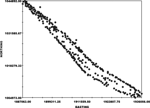
At first, the position of wells under study should be identified in the field (figure 1). Then the structural modelling of the Asmari Formation was done according to the following steps:

Figure 1 Location of wells in the field

1.	Define model.
2.	Fault modelling: In this stage, the extent of the fault in the field under study is specified.
3.	Pillar gridding: In this step, the network size should be determined. Note that these dimensions should be properly selected; if the dimensions are large, the results are not favourable and if the dimensions are small, the runtime of the model design will be too long.
4.	Making the horizons.
5.	Layering.

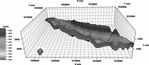
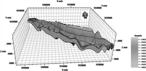
To determine the structural model of the Asmari Formation, first the top Asmari Formation data are analysed. Then, the data of upper and lower levels of the Asmari Formation are analysed and the surface for upper and lower levels of this formation is defined. After that, the fault model is determined, and then the layering of the three-dimensional model of the formation is plotted (figure 2).

Figure 2 Structural model of the Asmari Formation and the order of underlying layers

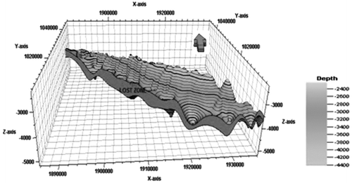
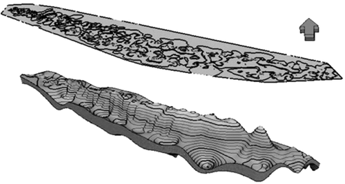
After determining the structural model of the Asmari Formation, to obtain the distribution model of loss in the Asmari Formation of the field under study, we must first determine the upper and lower surface of loss area using the drilling data and the wells drilled in this field, and then the layering of the 3D model of loss area is determined (figure 3). Since the loss usually occurs within the gaps and natural and induced fractures created in the structure of the Asmari Formation, the distribution model of the fractures and faults created in the loss area is also plotted (figure 4).

Figure 3 Distribution model of loss

Figure 4 Distribution of fractures and cracks in the loss area

In the final stage, the structural model of the loss distribution in the Asmari Formation of the field under study is designed three-dimensionally. Note that in this model, the loss area is marked by a light green colour (figure 5).

Figure 5 Distribution model of loss in the Asmari Formation

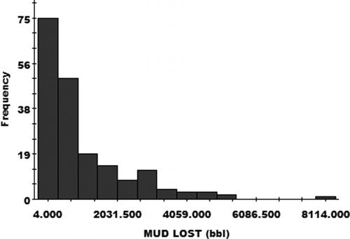
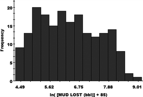
Mud loss is one of the problems usually encountered during drilling the Asmari Formation, causing many problems for us during drilling. The prediction of mud loss before entering the loss area for the drilling engineers is therefore of great importance. To predict the level of loss after the analysis of daily reports of 389 wells drilled in the field under study, the rate of mud loss for each of the wells in the Asmari Formation extent was specified. Data analysis, by drawing histograms and cumulative curves, is aimed to determine the type of distribution function and perform the necessary transformations to normalize it (before beginning estimation). After drawing the histogram, it can be seen that the data distribution is not normal (figure 6). To transform the data to normal, logarithmic method is used and the data histogram is plotted again (figure 7). After normalization, the cumulative frequency curve is checked. In this case, the cumulative frequency curve should be nearly a straight line (figure 8). Comparison of geostatistical parameters before and after normalizing the data is shown in table 1.

Table 1 Comparison of statistical parameters before and after normalization of data

Statistic parameter	Untransformed	Transformed
Mean	1021.5288	6.381
Std. deviation	1302.5776	1.148
Sample variance	1,696,708.3347	1.317
Minimum	4.000	4049
Maximum	8114.000	9.01
Skewness	2.01	0.19
Kortosis	4.92	−1.05

Figure 6 Non-normal distribution of data

Figure 7 Normal distribution of data

Figure 8 Cumulative frequency curve of data

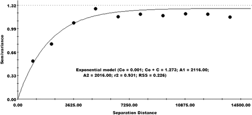
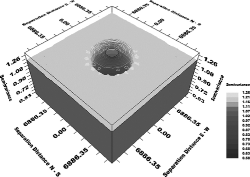
After normalizing the data, the spatial structure dominating the estimation space should be determined; at this stage, we draw the variogram. To plot the variogram, first the value of 2γ(h) (semivariance) for different distances of h (separation distance) in a diagram is plotted. The variogram in fact reflects the spatial correlation between data sets. After drawing the variogram, a model must be selected to fit the plotted variogram. The model selected for fitting should have minimum nugget effect and minimum sill with maximum effective range. In this study, after fitting different models and comparing the results (table 2), the model selected for fitting is the exponential model (figure 9). To observe the semivariance variations in different directions, the 3D model of the semivariance surface is plotted. It helps us determine the main axis of anisotropy in the variogram model (figure 10).

Table 2 Comparison of results from different model fittings

			Range Parameter		Effective Range
Model	Nugget C0	Sill C0 + C	Major A1	Minor A2	Major	Minor	Proportion c/(c0 + c)	r 2
Spherical	0.0010	1.2732	5014	4914	5014	4914	0.999	0.974
Exponential	0.0010	1.2732	2116	2016	6348	6048	0.999	0.931
Linear	0.8010	2.2632	39,120	39,070	39,120	39,070	0.646	0.478
Linear to all	0.8010	2.1012	34,780	34,710	34,780	34,710	0.619	0.478
Gaussian	0.9190	2.1912	22,730	22,640	39,369	39,213	0.581	0.305

Figure 9 Exponential model fitted

Figure 10 3D model of variogram surface

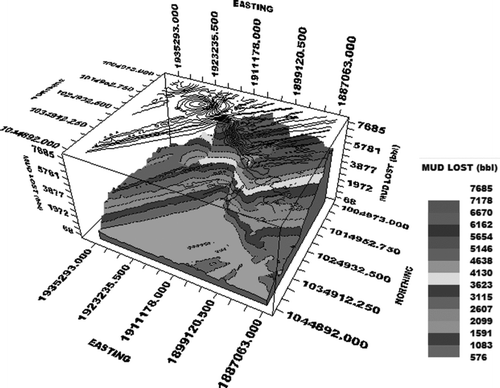
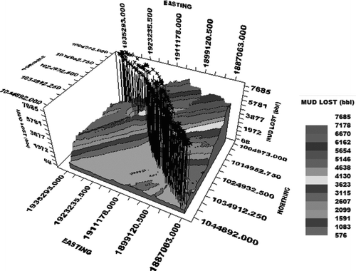
After determining the dominant spatial structure, we must select the appropriate estimator. Kriging is an estimation method according to the weighted moving average, and we can say that it is the best linear unbiased estimator (BLUE). One of the most important features of kriging is that for each error, the error associated with it can be calculated. Thus for each estimated value, we can calculate the confidence range. Search radius is an effective parameter in model design. In this model, the search radius is considered equal to the effective range. The number of points participating in the estimation of a point is a criterion for validity of the desired estimation. In the estimated value, a large number of data participate with different positions and affect it. The fewer the number of points, the less the probability of the estimated value to be affected by probable oscillations. As already mentioned, kriging has many types, and in this study block kriging has been used for model design. To increase precision in the estimates of block kriging estimates and reduce errors, the block size is differently presented. If the block size used in the estimation is smaller more spatial correlation between the data and the spatial structure is stronger. After a full implementation of the estimates, the three-dimensional model of estimation is presented (figure 11). For a better review of the wasting rate in the field under study, the position of wells in the prediction model of wasting rate is specified (figure 12).

Figure 11 3D model to predict the amount of mud loss in the Asmari Formation

Figure 12 Well location in the loss distribution model

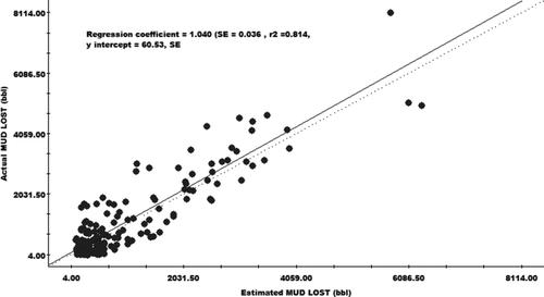
Cross validation is a method for controlling the error accuracy of estimation. In this method, the true value of data and the estimated value are placed close to each other on the same diagram, and the estimation error value is obtained by a comparison of these two values (figure 13). For testing the accuracy of this model, the position of the two wells drilled in which the wasting rate was known is compared with the designed model. This survey shows that the value of the estimated parameter is quite close to the actual value (table 3).

Table 3 Comparison between real value and estimated value by the model

Well number	Real value	Estimated value
Well 1	276	280
Well 2	3130	3145
Well 3	2545	2540
Well 4	5342	5335

Figure 13 Cross validation diagram for determining error estimation

7. Conclusions

The Asmari Formation is one of the most important formations for geologists and drillers in drilling oil wells in Iran. It is important because:

1.	Most of the oil reservoirs in this formation are located in the southern regions.
2.	In this formation, loss of drilling mud is relatively heavy.
3.	Determination of the top level of this formation with the purpose of designing casing.

Estimation is one of the most basic methods for studying the parameters of hydrocarbon reservoirs. The reason for this is the lack of data in all points of the reservoir. Geostatistics-based methods of estimation and simulation are widely accepted for simulation of different characteristics of hydrocarbon reservoirs, so that much of the modelling software in the field of evaluating oil and gas reservoirs, and in the field of earth sciences in general, operates based on these methods.

Geostatistical methods, especially kriging, are among the best estimators to study the variable parameters of the reservoir, and the models presented using geostatistical methods (particularly kriging) are highly accurate.

The model presented for predicting the mud loss volume enables us to predict the volume of mud losses in the reservoir rock before entering the loss area, and according to the loss volume, choose the right LCM (lost circulation materials). By accurately predicting the wasting volume and applying the appropriate treatments regarding the loss volume, penetration of solids in the mud into the formation is prevented, and damage caused by the entry of these solids into the production area is minimized.

Acknowledgements

The author thanks National Iranian South Oilfields Company (NISOC) for their help and financial support for any data and software.

References

- Corstange , R , Grunwald , S and Lark , R M . 2008 . Inferences from fluctuations in the local variogram about the assumption of stationary in the variance . Geoderma , 143 : 123 – 132 . doi: 10.1016/j.geoderma.2007.10.021
- Cressie , N and Hawkins , D M . 1980 . Robust estimation of the variogram . Math Geol , 12 ( 2 ) : 115 – 125 . doi: 10.1007/BF01035243
- Deutsch , C V . 2002 . Geostatistical reservoir modeling , 376 Oxford : Oxford University Press .
- Dimitrakopoulos , R and Desbarats , A J . 1997 . Geostatistical modeling of grid block permeabilities for 3D reservoir simulators . SPE Reservoir Eng. , 8 : 13 – 18 .
- Haining , R . 2003 . Spatial data analysis: theory and practice , Cambridge : Cambridge Uni-versity Press .
- Isaak , E H and Serivaster , R M . 1989 . An introduction to applied geostatistical , 561 Oxford : Oxford University Press .
- Jennings , J W Jr. , Lucia , F J and Ruppel , S C . 2002 . “ 3D modeling of stratigraphically controlled petrophysical variability in the South Wasson Clear Fork reservoir ” . In SPE Annual Technical Conference and Exhibition San Antonio 29 Sep–2 Oct, Texas SPE Paper No. 77592
- Kelsall , J and Wakefield , J . 2002 . Modeling spatial variation in disease risk: a geostatistical approach . J Am Stat Assoc. , 97 : 692 – 701 . doi: 10.1198/016214502388618438
- Mansuri , A J . 2002 . “ Polyurethane grouting geothermal lost circulation zones ” . In Paper IADC/SPE 74556. Paper presented at the IADC/SPE Drilling Conference 26–28 Feb Dallas, Texas
- Ortiz , C J and Deutsch , C V . 2002 . Calculation of uncertainty in the variogram . Math Geol , 34 ( 2 ) : 169 – 183 . doi: 10.1023/A:1014412218427
- Rueda , F . “ In-situ reactive system stops lost circulation and underground flow problems in several southern Mexico wells ” . In Paper SPE 59059, presented at the International Petrolum Conference and Exhibition Mexico 1–3 Feb
- Webster , R and Oliver , M A . 2007 . Geostatistics for environmental scientists. Statistics in practice , Chichester : Wiley .