Himalayan hazard study on the basis of stress and strain state of 1991 Uttarkashi earthquake using Coulomb stress transfer model

Abstract

Uttarkashi region of Himalaya was struck by a destructive earthquake (M_w = 6.8) on 19 October 1991 with its epicentre located at 30.78°N latitude and 78.77°E longitude.

Here, we use Coulomb stress model for the study of this major event. Coulomb 3.1 application is used to generate the earthquake model and develop the stress change maps of the region. The 1991 Uttarkashi earthquake and succeeding earthquakes of M_b > 3.5 are used for the study. One of the motives of this work is to correlate the main shock and the successive minor earthquakes that have occurred in the region. Further, we have studied the 1999 Chamoli earthquake using this model and attempted to relate its occurrence with the Uttarkashi earthquake based on propagation of strain energy.

The study of Uttarkashi 1991 earthquake by this method supports the main shock and its controlling effect on the later earthquakes’ observations in the nearby region with the view that many zones of such shock can occur in the future. This model is also used to predict the direction of propagation of strain energy, thereby locating the region that will be affected by the future shocks.

1. Introduction

The 19 October 1991 earthquake that occurred in the Garhwal Himalayan region is considered to be one of the most destructive earthquakes that occurred in India. The earthquake was found to be associated with a shallow – dipping thrust fault and the main rupture was found to occur at a depth of 10 km having the coordinates of 30.78°N latitude and 78.77°E longitude (Cotton et al. 1996). The Garhwal Himalayan region is highly prone to many destructive earthquakes in the past (Rastogi 1995) among which the 1803 earthquake of IX intensity on the Mercalli intensity scale was the most destructive (Smith 1843). Pradhan et al. (2006) and Dash et al. (2000) showed the probability is high for the occurrence of landslides in this region. They have mapped stress patterns using remote sensing data and attempted to relate this with the occurrence of the major earthquakes in this region. According to the online bulletin of International Seismological Centre (ISC), the Uttarkashi main shock was accompanied by many minor earthquakes of M_b > 3.5 that occurred for the next four months. Many methods have been used to study this earthquake, namely, rupture study using teleseismic data (Cotton et al. 1996), studying ground horizontal accelerations (Paul et al. 1998), analysis of strong motion data (Joshi 2006), studying the seismicity pattern (Wason 2010), analysing the regional tectonic model (Kayal 2010) and b-value and fractal dimension based study (Ghosal et al. 2012). Gahalaut (2012) stated that most of the earthquakes in this region have surprised us by generally not fitting properly to any defined method. Here, we study the 1991 Uttarkashi earthquake using the theory of Coulomb failure function (CFF), which is based on the study of stress state of the regional faults. Rajput et al. (2005) studied this event in their brief analysis of the major earthquakes of India based on Coulomb stress model. Further we have extended this work by using this method to understand the relation between the several earthquakes and the direction of propagation of related strain energy.

When the stress goes beyond a particular value known as critical stress, deformation and fracture formation occurrence takes place which in turn leads to reduction of stress. Many of the past works suggest that increase in the value of stress triggers the aftershocks as well as several other earthquakes that in the nearby region (Smith & Van de Lindt 1969; Hamilton 1972; Rybicki 1973; Yamashina 1978; Das and Scholz 1982). Thus, both the components, i.e. shear and normal stress changes, are combined under the name of Coulomb stress change. Thus studying the redistribution of strain energy based on Coulomb stress transfer model helps in understanding the direction of propagation of the seismic events in that region. This theory has been successfully applied to study many large earthquakes and is found to produce good results (Harris 1998; Voisin et al. 2004).

Here, we have done the study over a rectangular area encompassing the region bounded by 30°N and 31.5°N latitudes and 78°E and 79.5°E longitudes. The rectangular space is further divided into small grids having dimensions of 0.05° latitude × 0.05° longitude. This method is based on the assumption that the Coulomb stress change for each and every point lying inside a grid is same. Coulomb 3.1 (Toda et al. 2007), a graphic rich deformation and stress change software, is used to generate the grids and study the stress change and propagation of strain energy in the study region. The rectangular area was decided based on various factors. Considering a large study area will lead to increase in the differential area enclosed in each grid, hence leading to reduced resolution of output. Limiting the study to a very small area will cause for skipping the nearby areas that were affected by the aftershocks. This will lead to improper analysis of aftershocks, thus making it difficult to deduce proper conclusions. To obtain the stress and strain maps and the output files from the software, an initial input file needs to be build with desired input parameters (Toda et al. 2007). After supplying the input parameters, the shear, normal and Coulomb stress maps are generated. A file is created that holds the magnitude of Coulomb stress change for each grid. The source mechanism parameters of the earthquake are taken from the catalogues of USGS, PDE, Harvard, NEIC and ISC.

The stress state of the regional faults is studied to understand the effect of 1991 earthquake. Also, the aftershocks’ plot is made corresponding to the events that occurred for around six months in the region. All the events in the study area occurred after the main event of Uttarkashi earthquake, hence attempt of comparative study done with some of the later major shocks of the region such as the Chamoli 1999 earthquake. The various plots generated are further used to study the direction in which the aftershocks propagated. It also helped to understand the stress state of the region and find the region that was probable to future shocks.

2. Seismotectonic setting of the region

The Uttarkashi earthquake of 19 October 1991 occurred in the Garhwal Himalayan region of northern India (Wason 2010). This region lies at the collision junction of the Indian plate and Asian plate. As per the global plate tectonic models, the Indian plate is moving at the rate of 5 cm per year relative to the Asian plate in the north-east direction (Yu et al. 1995). Sahoo et al. (2000) presented a seismotectonic study of the region based on remote sensing and GIS studies that give a key to understanding of tectonics. The region is bounded by the Alaknanda River on the east and Tons River on the west. The tectonic features of this region are found to be striking along north-west–south-east direction (Valdiya 1976; Fuchs and Sinha 1978; Wason 2010). The major northward dipping thrust in this region is main central thrust (MCT). However in Uttarkashi region, problem is very complex as it is difficult to precisely locate the MCT. Ni and Barazangi (1984), Baranowski et al. (1984) and Khattri (1987) have already studied the seismicity in the region. The thrust planes are found to be inclined at about 30^o or 40^o to the horizontal (Valdiya 1980).

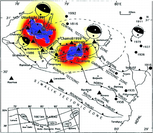
As per the previous studies, the region lying between the MCT and main body thrust (MBT) is highly prone to moderate earthquakes (Molnar et al. 1973; Chandra 1978; Seeber et al. 1981). The earthquakes in the region are shallow focused and are generally found to lie within 20 km of the crust (Baranowski et al. 1984; Ni & Barazangi 1984). The fault plane solutions for the events of this region are found to be characterized by reverse faulting mechanism with a small slip component in the strike direction (Wason 2010). Figure 1 shows the focal mechanism of the 1991 Uttarkashi earthquake, 1999 Chamoli earthquake and also the epicentres of some of the smaller events of the region. The fault plane solution of the main shock shows low angle thrust faulting and the aftershocks show thrust faulting as well as strike-slip faulting to some extent. The main shock and the aftershocks for the Uttarkashi earthquake are found to lie above the plane of detachment (Kayal 2007).

Figure 1. Tectonic map of the Garhwal Himalayan region showing the focal mechanisms of 1991 Uttarkashi earthquake, 1999 Chamoli earthquake and a few other major events of the region. It also shows the epicentres of all the major earthquakes that have occurred in the study area. Coulomb stress change has been shown for Uttarkashi and Chamoli earthquakes, where blue colour (for negative change) and red colour (for positive change) are used to denote the variations of stress change in a graphical manner (modified after Yeats and Thakur 1998).

3. Coulomb stress change and its determination

Earthquake causes for change in the stress and strain state of the faults of the region of occurrence. The amount of stress change produced in a fault or a series of faults can be helpful to predict the occurrence of a future earthquake. When the stress change exceeds a critical value, fractures develop with the release of strain energy to take the fault to its stable state. In the seismogenic faults, the stability of fault depends on the frictional force as well as the shear stress applied to it and is given by Navier–Coulomb failure criteria (Jaeger & Cook 1976):(1) where τ is known as shear stress, σ is the normal stress, μ is the coefficient of friction and s is the internal adhesive force on the given fault plane. Let σ_f = τ − s − μσ, where σ_f is the Coulomb stress that decides the stability of fault. Because of mutual interaction between different faults, an earthquake results into change of the shear stress τ and normal stress σ on its surrounding faults, thereby causing their Coulomb stress to change. Since these stress change are generated as same time as other earthquake occurrence, they are called coseismic Coulomb stress change.

As per the formula (1), in order to obtain the Coulomb stress changes on fault, the changes of shear and normal stress on it should be calculated. The resultant of shear and normal stress determines the co-seismic Coulomb stress. Hence, the calculation of coseismic Coulomb stress change shortens down to the problem of stress changes on faults resulted from the slip, creeps and displacement on the seismogenic fault. Theoretically, the co-seismic Coulomb stress change caused by fault interaction is affected by both static and dynamic stress. Though the shear and normal stresses are functions of time, at larger distances from the epicentre, they approach a static configuration (Harris & Day 1993; Cotton & Coutant 1997; Belardinelli et al. 2003). Also, the transfer of stress caused due to dynamic processes is complex and difficult to study; hence, in most cases, only static stress triggering is considered in coseismic Coulomb stress change. The theory of static stress displacement is an effective tool to handle this type of problem. For the past decade, much work has been done to study the static stress field resulted from the displacement in crust. Especially, Okada (1985, 1992) developed a method to study the surface and internal deformation due to shear and tensile faults in a half-space, by which a series of mathematical problems were solved. It has become the classical algorithm to process the surface and internal deformation caused by fault displacement (Gomberg & Ellis 1993; King et al. 1994). The displacements produced in the region due to the main shock along and across the fault were studied to understand the direction of propagation of the aftershocks. Further, to analyse the stress change produced on the regional fault, the workflow can be summarized as follows:

1. Manipulation of the external boundary conditions: The external boundaries conditions refer to the regional tectonic stress field, strain field or displacing the field, and have been obtained using the Coulomb 3.0 and the fault parameters obtained from USGS.

2. Deciding the internal boundary conditions: The stress, strain or relative displacement is included in the internal boundary conditions. These can be obtained by means of observation, geodesy or experiential formulas and so on.

3. The calculation of stress, strain or displacement produced on the faults around the seismogenic fault.

4. The calculation of coseismic Coulomb stress change caused by fault interaction.

As per the Navier–Coulomb failure criteria, the change produced on the Coulomb shear stress shortens (or lengthens) the time required for regional stress to bring it to failure. When a fault is close to failure, increasing its Coulomb stress may trigger an earthquake on the fault immediately. If the fault is far away from the failure, the increase of Coulomb stress can also accelerate its stress accumulation and advance the time to the next earthquake. In reverse, decreasing the Coulomb stress on a fault segment causes its stress to be lower than the critical value of failure, and thus delays the next earthquake occurrence. (Stein et al. 1992, 1997; Zhang et al. 2001). Currently, this method is widely applied to quantitatively assess the seismic risk of active fault. Hence, studying the stress state of the faults of a region before and after an earthquake can be helpful in predicting the future shocks. We have performed retrospective study of the Chamoli and Uttarkashi events and rather than performing quantitative assessment, we have tried to focus on qualitative study of the stress and strain maps and understand the direction of propagation of the seismic events of this region on a temporal scale.

4. Methodology

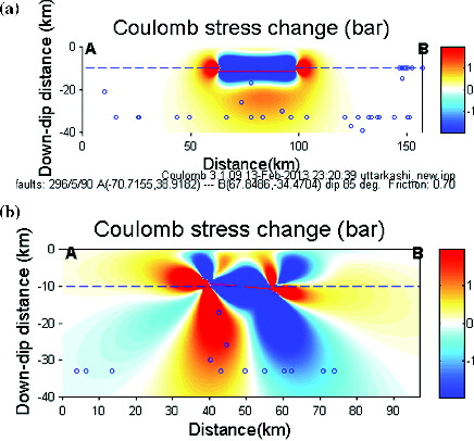
The graphic based Coulomb 3.1 application (Lin & Stein 2004; Toda et al. 2005, 2007) is used here for estimation of shear stress (figure 2(a)), normal stress (figure 2(b)) and Coulomb stress (figure 2(c)) along and across the rupturing fault in order to study the potential of the future earthquake on the nearby faults. Figure 3(a) and (b) shows the vertical cross-sectional maps of Coulomb stress changes along and across the fault plane. The coefficient of fault friction was considered to be 0.7 for thrust fault system (Scholz 2002).

Figure 2. Plot of showing the stress states of the region after the 1991 Uttarkashi earthquake and 1999 Chamoli earthquake. Blue colour denotes reduction and red denotes accumulation of stress in the plots of (a) shear stress (b) normal stress (c) Coulomb stress with main aftershocks and earthquakes with M_b > 3.5 for Uttarkashi earthquake and (d) coulomb stress for Chamoli earthquake.

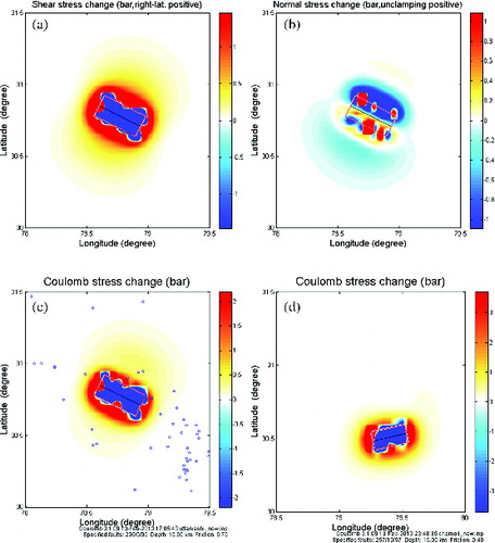
Figure 3. Vertical cross-sectional plot of the Coulomb stress change for the Uttarkashi 1991 earthquake (a) along the fault fracture (b) across the fault fracture.

The magnitude of the main event is used as per USGS database (M_w 6.8). In addition to studying the stress state of the regional faults, the main aftershocks and some minor earthquakes with M_b > 3.5 are plotted for the study area for two different time intervals: one just after 6 months of the main shock (figure 4(a)) and another for all the events that have occurred in the region after the Uttarkashi main shock (figure 4(b)). The study of both these plots simultaneously gives the idea about the direction of propagation of these events. The data for these plots is obtained from ISC database. The 90° rake and 5° slip (fault input parameters) are obtained from the USGS focal mechanism. Also, strain maps denoting strain produced across various planes and displacement plots of the region are generated.

Figure 4. Plots showing the events with M_b > 3.5 that have occurred after the Uttarkashi earthquake in the nearby region for (a) next six months of the main shock (b) till date after the main shock.

5. Study of Coulomb stress change

Any earthquake, either moderate or strong, leads to change in stress state of the faults of the associated region. The stress change produced by the main shock does not necessarily cause all the faults to attain the stable state. Some of the faults enter unstable state; hence, aftershocks or some future earthquakes are needed for their stability. This is one of the main reasons for the cause of the seismic events in the near future after the main shock has occurred. The point of origin of the future shock will be decided by the points of accumulation of strain energy during the main event. Thus, studying the Coulomb stress change maps can help in predicting the region that is probable to the future shocks. Stein (1999) studied the role of stress transfer in the occurrence of earthquakes. Several researchers have studied the stress change and the effects in major faults within 100 km of the Loma Priesta, California shock (Reasenberg & Simpson 1992; Simpson & Reasenberg 1994; Parsons et al. 1999). Cocco et al. (2000) studied the 1997 sequence of eight shocks of the Umbria-Marche region of Italy and found them to have been promoted by stress change caused during the Landers earthquake. Hardebeck et al. (1998) used the Coulomb stress transfer model to study the Landers and Northridge earthquakes. Cakir et al. (2003) used this method to study the 1999 Izmit and Duzce earthquakes of the Marmara region and deduced that Izmit and other events of the region triggered the Duzce earthquake. Rajput et al. (2005) used this method to assess the seismic hazard for several Indian earthquakes such as 2001 Bhuj earthquake, 1999 Chamoli earthquake, 1997 Jabalpur earthquake, 1991 Uttarkashi earthquake, etc. In this paper, we use this method to study the 1991 Uttarkashi earthquake and further try to relate the 1999 Chamoli earthquake with this event.

The epicentre of the main shock is considered to lie at the centre of the fault plane; hence, for a small dip of the fault plane as in this case, there is almost a uniform stress drop on sides of the rupture. Figure 2 (a)–(c) shows the static, dynamic and Coulomb stress change due to the Uttarkashi main event. The stress change for each grid is calculated using the Navier's method of stress determination (Bizzarri 2010). Blue (for negative change) and red colour (for positive change) are used to denote the variations of stress changes in a graphical manner. Figure 2(a) clearly shows the region of relaxed faults marked by negative change (blue colour) during the Uttarkashi 1991 earthquake, indicating the release of stored strain energy, causing for a decrease in the magnitude of the shear stress of the associated faults. These faults attained relaxed state while developing a tension force in the region nearby. Hence, the shear stress of the nearby region is increased, increasing the probability of aftershocks in the nearby region. But shear stress change is not the only one to govern the future shocks. Figure 2(b) shows the change in normal stress in the given region. There is a positive change (red colour) in normal stress in the adjoining region while negativity (blue colour) is seen near the rupture area. An increase of about 1 bar of pressure can be seen in the region adjoining Uttarkashi. The normal stress at the rupturing fault decreases due to the release of energy. Thus, the upper crust in this region relaxes, a compressive force acts towards the adjoining region. The resultant stress produced as a sum of shear and normal stress is represented by Coulomb stress change (figure 2(c)). The Coulomb stress change is plotted together with some of the main aftershocks and the minor earthquakes that have occurred in this region after the 1991 Uttarkashi earthquake. A resultant drop in Coulomb stress is seen near the main event while there is an increase of Coulomb stress in the surrounding region. However, the increase in magnitude of the Coulomb stress in the nearby region is not sufficient to cause for a major future shock in the region. But a small rupture or a shock in future may be sufficient enough to help these faults attain the condition of Coulomb failure, causing for the occurrence of seismic events in these region. Figure 2(d) shows the Coulomb stress change plot for the 1999 Chamoli earthquake. The events that have occurred after the Uttarkashi main event are in agreement with the stress change map of Chamoli earthquake. This event together with the fault rupture direction lies in the line of propagation of the seismic events that have been moving from the Uttarkashi earthquake towards the south-east direction.

In addition to the stress maps, we performed the study of displacement maps and strain plots for our study area and tried to correlate them with the events that succeeded the Uttarkashi event. Again from the Coulomb stress change, we see that all the areas surrounding the Uttarkashi area also experience almost equal amount of stress change. But generally, the stress accumulation at the two nodes is more; thus, slightly modified stress state is seen at the two nodes. Hence, the probable directions of propagation of future events are towards north-west as well as south-east. We use vertical cross-sectional view of Coulomb stress change in along the width and length of the fault (figure 3(a) and (b)). It is seen that the region lying towards point A in figure 3(b) is more probable to aftershocks due to increased stress accumulation in the region. There are some chances that the aftershocks might have propagated towards the south, and as the stress accumulation is maximum at the nodes, the most probable direction is towards south-east. The study of strain and displacement maps is discussed in the next sections. The results obtained here are compared with the aftershock's plot of the region. The aftershocks’ plot of six months (figure 4(a)) shows some of the major aftershocks that occurred in the region after the Uttarkashi main shock. The aftershocks are mainly found to be concentrated towards the south of this region and are randomly distributed in east as well as west direction. But they are not clearly distributed in one direction, because the stress change brought by the main shock is not aligned in one particular direction but is distributed to all parts. But as we move on temporal scale, we find that the number of aftershocks increase in the south-east direction and hence define a direction of propagation (figure 4(b)). We are not able to find this thing from the stress maps, because they only consider the stress change due to the main shock and not even the major aftershocks. The figure 4(b) showing the shocks for a long period of time after the main shock of Uttarkashi clearly indicates that the energy has been travelling towards south-east. The 1999 Chamoli earthquake that occurred to the south-east of Uttarkashi event can be said to have been triggered by it. Hence, Coulomb stress model is successful to some extent in defining the correct stress state of the regional faults and indicating the right direction for the propagation of the aftershocks.

6. Effect of Coulomb stress change on future earthquakes

An earthquake affects the static stress state of the regional crust. Coulomb stress changes denote how much a nearby fault has been dragged to the condition of rupture or the extent to which it has attained a relaxed state. By studying it, we can have the idea whether the occurrence of the next earthquake event in this region has been triggered or delayed.

The study involved in this paper is completely based on the main shock and in addition the triggering or delaying effect of only the main shock has been studied. We have taken this assumption for the following reasons: the magnitude of main shock is much larger than the aftershocks; main shock, while causing for release of strain energy in a region, also brings the faults of the nearby region to more stressed state, while aftershock's affect on the faults at some distance from its occurrence is negligible. This reduces the complexities of the model and makes it easier to interpret it and predict the occurrence of future earthquakes. In the last section, we derived an idea that the probable direction of aftershocks’ occurrence is towards the south-east of the main shock that is supported by the results from the aftershocks’ plots. The occurrence of 1999 Chamoli earthquake event also supports the analogy of predicting the direction of propagation of the future shocks. Chamoli earthquake is also one of the devastating events that shook the entire Garhwal region. This earthquake occurred to the south-east of the Uttarkashi event after eight years. The epicentre of this event lies on the line of propagation of the seismic events that caused for the 1991 Uttarkashi earthquake. Due to the Uttarkashi earthquake, the nearby region of Uttarkashi is expected to have had experienced a Coulomb stress change of about 1 bar. Though this stress change may not be enough to trigger a big event, it may cause of aftershocks that help in further propagation of strain energy away from the epicentre of the main event. The energy keeps on propagating and the direction of propagation of strain energy is generally along the fault. This fact is observed in the Uttarkashi event too. When this propagating energy meets a fault that is under high stress, it causes for the rupturing of the fault leading to a major event. In this way, Coulomb stress transfer model can be used to relate several major earthquakes occurring in a small region. We have applied this theory over the Uttarkashi earthquake and it is found that the Uttarkashi event itself is the result of triggering caused by some major events that occurred in past in the Garhwal Himalayan region.

7. Comparison of 1991 Uttarkashi and 1999 Chamoli earthquakes

Both of these earthquakes occurred in the central gap region of the Himalaya between the MCT and MBT. The fault plane solutions of both the events suggest that the dominant deformation model for both events is low-angle north-easterly dipping thrust faulting. The earthquake parameters associated with both the events are given in table 1. Both of these are moderate earthquakes and Khattri et al. (1989) indicated that moderate earthquakes occur in this region due to the reactivation of the low-angle thrust faults in the upper crust parallel to the detachment surface. The Uttarkashi earthquake showed the thrust faulting, with shallow dipping aftershocks. Similarly, Chamoli earthquake had thrust faulting mechanism with aftershocks showing thrust and strike-slip faulting to some extent (Kayal et al. 2003). When aftershocks’ plots of both these events are visualized separately, it can be seen that in both of these plots, there are two clusters of aftershocks, one lying towards the north-west and the other towards south-east of the epicentres of the respective events. But, one thing is found common from both the plots, i.e. if both of these plots are seen on the same map, it can be seen that the aftershocks form a linear chain with the main events lying on this line. From the Coulomb stress maps of Uttarkashi and Chamoli events (figure 2(c) and (d), respectively), we see that direction of stress propagation is same for both the events. It can be inferred that both of these earthquakes are a part of a series of earthquakes that have been occurring in the Garhwal Himalaya region. Hence, Uttarkashi can be considered an after event of the past earthquakes of the region, and Chamoli event as the successor of the Uttarkashi event. The Chamoli earthquake occurred long time after the Uttarkashi earthquake and it lies towards the south-east of Uttarkashi. Hence, it can be concluded, to some extent, that if these series of earthquakes are considered to be propagating, then the direction of propagation will be south-east.

Table 1. Source Parameters for the 1991 Uttarkashi earthquake and 1999 Chamoli earthquake from USGS, PDE and Harvard catalogues denoting the plunge and azimuths for the three principal axes and strike, dip and slip for the two nodal planes.

	Principal axis						Nodal planes
	T		N		P		1			2
Earthquake event name	PL	AZ	PL	AZ	PL	AZ	STK	DIP	SLIP	STK	DIP	SLIP	Source
Uttarkashi	38	351	37	118	30	235	296	5	90	1116	85	90	PDE
Uttarkashi	57	14	6	113	32	207	317	14	115	112	78	84	HRV
Chamoli	53	27	5	290	37	196	257	10	57	111	82	95	USGS
Chamoli	52	27	2	295	38	203	280	7	75	115	83	92	HRV

8. Analysis of strain and crustal displacement in the region

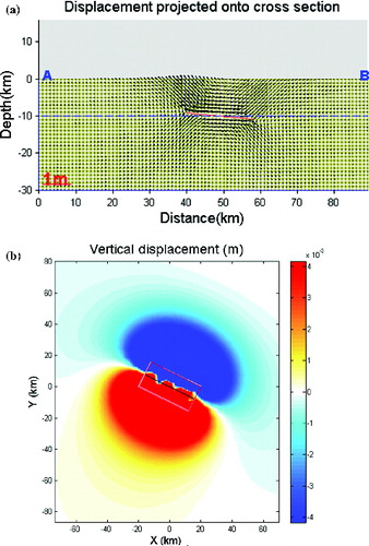
We have tried to study the displacement of the crustal points of the region and understand the distribution of strain caused by the Uttarkashi earthquake. Further Coulomb 3.1 is used to generate the strain and displacement maps of the region. The vertical displacement map is also generated that gives the vertical movement of the surface during the rupture. This map helps in understanding the type of faulting associated with the earthquake. The displacement map gives the idea of how much the surface in a region was elevated or went down (figure 5). The line AB is drawn across the fault. While the region towards the point A is found to be elevated, the opposite side is found to go down. The displacement shown is very small such that even the points lying very close to the ruptured fault show a displacement of about 15 cm. A relative scale is shown in figure 5(a), which denotes a metre length. The displacement of a point can be approximated by comparing the length of the concerned arrow with the metre length arrow. Figure 5(b) uses colour variation to denote vertical displacement. While red colour denotes positive displacement (elevation), blue is used as the convention for negative displacement.

Figure 5. (a) Vertical cross-sectional view of the displacement of the crust. Points A and B are two points on the surface of the earth used for indicating the relative displacement. The arrow at the left bottom indicates l m length. Arrows indicating displacement can be compared with these to get the approximate displacement of a point. (b) Displacement map of the region enclosing the epicentre of the 1991 Uttarkashi earthquake immediately after the main event. Red colour denotes positive vertical displacement (elevation) and blue denotes that the point went down.

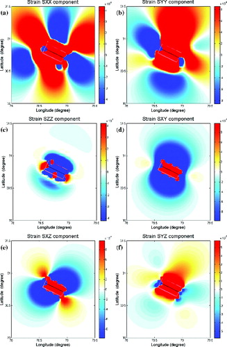
The strain maps obtained from the Coulomb 3.1 software give an idea of the strain produced in the region. The accuracy of strain estimation depends on the number of grids used in the study area. Coulomb 3.1 does not give strain approximation for every differential point of the region; rather it assumes a constant value for every point lying in the same grid. Hence, more the number of grids defined, lesser will be extrapolation and more will be the accuracy. A 3D model of the region is analysed, where each point (each small grid) is represented in the form of p (x, y, z). The strain tensor is analysed with respect to all its six components, out of which three normal components and rest three components are mainly of the shear strain. S_xx, S_yy and S_zz are the normal components of strain towards x-, y- and z-directions, respectively. Figure 6(a)–(c) represents the three components of the normal strain. Blue represents the area of negative strain, while red is used to indicate positive strain. Similarly, figure 6(d)–(f) represents the components of the shear strain S_xy, S_xz and S_yz lying in the xy, xz and yz planes, respectively. Same colour conventions (red and blue) of representation have been used in this case also. The areas that go under highly compressed state are most probable to be affected by a future earthquake. As in this representation, it is found that the magnitude of negative strain in the south-east direction of Uttarkashi is high. Not only is negative strain necessary for a future shock but also a large positive change in the value of strain can also cause for events in the future. Thus, a small positive change in Coulomb stress in future is sufficient enough to change level of strain for the regional fault for the cause of rupture.

Figure 6. Normal Strain produced along the (a) x-direction (b) y-direction (c) z-direction and the shear strain produced in the (d) XY plane (e) XZ plane (f) YZ plane (positive change denoted by red and negative by blue colour) for 1991 Uttarkashi earthquake.

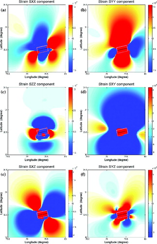
In addition to the Uttarkashi event, we have also studied the strain maps for the 1999 Chamoli earthquake. Figure 7(a)–(c) represents the three components of the normal strain for the Chamoli event and figure 7(d)–(f) represents the components of the shear strain S_xy, S_xz and S_yz lying in the xy, xz and yz planes, respectively. We find that the strain maps of the Chamoli earthquake show approximately the same response as that of the Uttarkashi event, thereby denoting the propagation of strain energy along the north-west–south-east direction.

Figure 7. Normal Strain produced along the (a) x-direction (b) y-direction (c) z-direction and the shear strain produced in the (d) XY plane (e) XZ plane (f) YZ plane (positive change denoted by red and negative by blue colour) for 1999 Chamoli earthquake.

9. Conclusions

Uttarkashi (1991) earthquake along the fault lying near MCT is a seismogenic sequence that is continuous temporally. We used Coulomb stress model for the study of this event and it shows good results that show resemblance with the past research works. The earthquake occurred due to the increase of the Coulomb stress, which resulted from the past earthquakes of the region. Also, this earthquake led to increase of Coulomb stress along the various associated faults of the region. The main event caused for sudden change of stress state of the nearby region and hence increased the stress accumulation in the nearby region. But the stress distribution was random and was seen in all directions. As the rupture was aligned along north-west south-east direction, the accumulation of stress was considered maximum in this direction, based on the concept that maximum stress accumulation happens along the fault rupture. The aftershock's plots confirmed the fact that the maximum stress accumulation was towards the south-east of the epicentre of Uttarkashi event. It was found that the 1999 Chamoli earthquake was triggered by this event. Hence, we correlated the 1999 Chamoli event also with this event. Even it can be considered that both are the triggered effect of some past event and lie on the same temporal series. Also, displacement analysis and study of strains for various direction planes helped us to understand the change more clearly. Our coulomb stress model seems to fit well with the event and shows resemblance with past results. Using this model, we conclude that the Coulomb stress change is the key to probe into the effect of earthquake triggering and delaying caused by fault interactions.

Acknowledgements

Authors gratefully acknowledge the Ministry of Earth Science, Government of India, for sponsoring this work. NEIC, USGS and ISC are thankfully acknowledged for the data and Ross Stein and team are thanked for the Coulomb software. Moreover, we are thankful to anonymous reviewers for their valuable suggestions and support of Prof. Ramesh P. Singh, Editor, towards encouragement of this work. The Abdus Salam ICTP, Trieste, Italy, is acknowledged for Junior Associate support to PNSR for completing the revision.

References

- Baranowski J, Armbruster J, Seeber L, Molnar P. 1984. Focal depths and fault plane solutions of earthquakes and active tectonics of the Himalaya. J Geophys Res. 89:6918–6928.
- Belardinelli ME, Bizzarri A, Cocco M. 2003. Earthquake triggering by static and dynamic stress changes. J Geophys Res. 108:2135–2150.
- Bizzarri A. 2010. Toward the formulation of a realistic fault governing law in dynamic models of earthquake ruptures. In: Brito AV, editor. Dynamic modelling. Croatia: INTECH; p. 167–188.
- Cakir Z, Barka AA, Evren E. 2003. Coulomb stress interactions and 1999 Marmara earthquakes. Turk J Earth Sci. 12:91–103.
- Chandra U. 1978. Seismicity, earthquake mechanisms and tectonics along the Himalayan mountain range and vicinity. Tectonophysics. 16:109–131.
- Cocco M, Nostro C, Ekstrem G. 2000. Static stress changes and fault interaction during the 1997 Umbria-Marche earthquake sequence. J Seismol. 4(4):501–516.
- Cotton F, Campillo M, Deschamps A, Rastogi BK. 1996. Rupture history and seismotectonics of the 1991 Himalaya earthquake. Tectonophysics. 258:35–51.
- Cotton F, Coutant O. 1997. Dynamic stress variations due to shear faults in a plane layered medium. Geophys J Royal Astron Soc. 50:643–668.
- Das S, Scholz K. 1982. Off fault aftershock clusters caused by shear stress increase? Bull Seismol Soc Am. 7:1669–1675.
- Dash P, Singh RP, Voss F. 2000. Anomalous stress pattern in Chamoli region observed from IRS-1B data. Curr Sci. 78:1066–1070.
- Fuchs G, Sinha AK. 1978. The tectonics of the Garhwal-Kumaun lesser Himalaya. J Geol. 121:219–241.
- Gahalaut VK. 2012. Great earthquakes as ‘surprises’ of our lack of understanding. Curr Sci. 102:1508–1509.
- Ghosal A, Ghosh U, Kayal JR. 2012. A detailed b-value and fractal dimension study of the March 1999 Chamoli earthquake (Ms 6.6) aftershock sequence in western Himalaya. Geomatics, Nat Hazards Risk, 3:271–278.
- Gomberg J, Ellis M. 1993. 3D-Def: A User's Manual. USGS open-file report. 93–547.
- Hamilton RB. 1972. Aftershocks of the Borrego mountain earthquake from April 12 to June 12, 1968, in The Borrego mountain earthquake of April 9, 1968. US Geological Survey Professional Paper. 787:31–54.
- Hardebeck JL, Nazareth JJ, Hauksson E. 1998. The static stress change triggering model: Constraints from two southern California aftershocks sequences. J Geophys Res. 103:24427–24437.
- Harris RA. 1998. Introduction to special section: Stress triggers, stress shadows, and implications for seismic hazard. J Geophys Res. 103:347–324.
- Harris RA, Day SM. 1993. Dynamics of fault interaction: Parallel strike slip faults. J Geophys Res. 98:4461–4472.
- Jaeger JC, Cook NHW, editor. 1976. Fundamentals of rock mechanics. London: Chapman and Hall Press; p. 1–56.
- Joshi A. 2006. Analysis of strong motion data of the Uttarkashi Earthquake of 20th October 1991 and the Chamoli Earthquake of 28th march 1999 for determining the Q value and source parameters. ISET J Earthquake Technol. 468:11–29.
- Kayal JR. 2007. Recent large earthquakes in India: Seismotectonic prospective. Int Assoc Gondwana Res Memoir. 10:189–199.
- Kayal JR. 2010. Himalayan tectonic model and the great earthquakes: An appraisal. Geomatics, Nat Hazards Risk. 1:51–67.
- Kayal JR, Ram S, Singh OP, Chakraborty PK, Karunakar G. 2003. Aftershocks of the March 1999 Chamoli earthquake and seismotectonic structure of the Garhwal Himalaya. Bull Seismol Soc Am. 93:109–117.
- Khattri KN. 1987. Great earthquakes, seismicity gaps and potential for earthquake disaster along the Himalaya plate boundary. Tectonophysics. 138:79–92.
- Khattri KN, Chander R, Gaur VK, Sarkar I, Kumar S. 1989. New seismological results on the tectonics of the Garhwal Himalaya. Proc Indian Acad Sci Earth Planetary Sci. 98:91–109.
- King GCP, Stein RS, Lin J. 1994. Static stress change and the triggering of earthquake. Bull Seismol Soc Am. 84:935–953.
- Lin J, Stein RS. 2004. Stress triggering in thrust and subduction earthquakes, and stress interaction between the southern San Andreas and nearby thrust and strike-slip faults. J Geophys Res. 109, B02303:1–19.
- Molnar P, Fitch TJ, Wu FT. 1973. Fault plane solutions of shallow earthquakes and contemporary tectonics in Asia. Earth Planet Sci Lett. 19:101–112.
- Ni J, Barazangi M. 1984. Seismotectonics of the Himalayan collision zone: geometry of the underthrusting Indian plate beneath the Himalaya. J Geophys Res. 89:1147–1163.
- Okada Y. 1985. Surface deformation due to shear and tensile faults in a half-space. Bull Seismol Soc Am. 75:135–154.
- Okada Y. 1992. Internal deformation due to shear and tensile faults in a half-space. Bull Seismol Soc Am. 82:18–40.
- Parsons T, Stein RS, Simpson RW, Reasenberg PA. 1999. Stress sensitivity of fault seismicity: A comparison between limited-offset oblique and major strike-slip faults. J Geophys Res. 104:20183–20202.
- Paul A, Sharma ML, Singh VN. 1998. Estimation of focal parameters for Uttarkashi earthquake using peak ground horizontal accelerations. ISET J Earthquake Technol. 372:1–8.
- Pradhan B, Singh RP, Buchroithner MF. 2006. Estimation of stress and its use in evaluation of landslide prone regions using remote sensing data. Adv Space Res. 37:698–709.
- Rajput S, Gahalaut VK, Sahu VK. 2005. Coulomb stress changes and aftershocks of recent Indian earthquakes. Curr Sci. 108:576–588.
- Rastogi BK. 1995. Seismological studies of Uttarkashi earthquake of October 20, 1991. J Geol Soc India. 30:43–50.
- Reasenberg PA, Simpson RW. 1992. Response of regional seismicity to the static stress change produced by the Loma Prieta earthquake. Science. 255:1687–1690.
- Rybicki K. 1973. Analysis of aftershocks on the basis of dislocation theory. Phys Earth Planet Inter. 7:409–422.
- Sahoo PK, Kumar S, Singh RP. 2000. Neotectonic study of Ganga and Yamuna tear faults, NW Himalaya, using remote sensing and GIS. Int J Remote Sensing. 21:499–518.
- Scholz CH. 2002. The mechanics of earthquakes and faulting. 2nd ed. Cambridge, UK: Cambridge University Press; p. 1–496.
- Seeber L, Armbruster J, Quittmeyer RC. 1981. Seismicity and continental subduction in the Himalayan arc. In: Gupta HK, Delany FM, editors. Zagros, Hindu Kush, Himalaya: Geodynamic Evolution, Geodynamic Series. Washington, DC: AGU; p. 215–242.
- Simpson RW, Reasenberg PA. 1994. The Loma Prieta, California, Earthquake of October 17, 1989. In: Simpson RW, editor. Tectonic processes and models. Professional Paper 1550-F, US Geological Survey; p. F55–F89.
- Smith LRB. 1843. Memoir on India earthquakes. J Asiatic Soc Bengal. 12:1029–1059.
- Smith SW, Van de Lindt W. 1969. Strain adjustments associated with earthquakes in southern California. Bull Seismol Soc Am. 59:1569–1589.
- Stein RS. 1999. The role of stress transfer in earthquake occurrence. Nature. 402:605–609.
- Stein RS, Barka AA, Dieterich JH. 1997. Progressive failure on the North Anatolian fault since 1939 by earthquake stress triggering. Geophys J Int. 128:594–604.
- Stein RS, King GCP, Lin J. 1992. Change in failure stress on the southern San Andreas Fault system caused by the 1992 Magnitude = 7.4 Landers earthquake. Science. 258:1328–1332.
- Toda S, Stein RS, Lin J, Sevilgen V. 2007. Coulomb 3.1 Software: USGS Stress Triggering Group.
- Toda S, Stein RS, Richards-Dinger K, Bozkurt S. 2005. Forecasting the evolution of seismicity in southern California–Animations built on earthquake stress transfer. J Geophys Res. 110(B05S16):17.
- Valdiya KS. 1976. Himalayan transverse faults and folds and their parallelism with subsurface structures of north Indian plains. Tectonophysics. 32:353–386.
- Valdiya KS. 1980. The two intracrustal boundary thrusts of the Himalaya. Tectonophysics. 66:323–348.
- Voisin C, Cotton F, Carli SD. 2004. A unified model for dynamic and static stress triggering of aftershocks, antishocks, remote seismicity, creep events, and multi-segmented rupture. J Geophys Res. 109(B06304):12.
- Wason HR. 2010. Post-1991 Uttarkashi earthquake seismicity pattern in the Garhwal Himalayan region. Proceedings for the 25th Himalaya-Karakoram-Tibet Workshop: US Geological Survey, Open-File Report. 1:2010–1099.
- Yamashina K. 1978. Induced earthquakes in the Izu Peninsula by the Izu- Hanto-Oki earthquake of 1974, Japan. Tectonophysics. 51:139–154.
- Yeats RS, Thakur VC. 1998. Reassessment of earthquake hazard based on a fault-bend fold model of the Himalayan plate-boundary fault. Curr Sci. 74:230–233.
- Yu G, Khattri KN, Anderson JG, Brune JN, Zeng Y. 1995. Strong ground motion from the Uttarkashi earthquake: comparison of observations with synthetics using the composite source model. Bull Seismol Soc Am. 85:31–50.
- Zhang Q, Wang C, Zhang P. 2001. Earthquake triggering and delaying caused by fault interaction. Proceedings of 2000’ Chinese Postdoctor Academic Conference, p. 354–359.