A study of waterborne diseases during flooding using Radarsat-2 imagery and a back propagation neural network algorithm

Abstract

Flood disasters are closely associated with an increased risk of infection, particularly from waterborne diseases. Most studies of waterborne diseases have relied on the direct determination of pathogens in contaminated water to assess disease risk. In contrast, this study aims to use an indirect assessment that employs a back propagation neural network (BPNN) for modelling diarrheal outbreaks using data from remote sensing and dissolved-oxygen (DO) measurements to reduce cost and time. Our study area is in Ayutthaya province, which was very severely affected by the catastrophic 2011 Thailand flood. BPNN was used to model the relationships among the parameters of the flood and the water quality and the risk of people becoming infected. Radarsat-2 scenes were utilized to estimate flood area and duration, while the flood water quality was derived from the interpolation of DO samples. The risk-ratio function was applied to the diarrheal morbidity to define the level of outbreak detection and the outbreak periods. Tests of the BPNN prediction model produced high prediction accuracy of diarrheal-outbreak risk with low prediction error and a high degree of correlation. With the promising accuracy of our approach, decision-makers can plan rapid and comprehensively preventive measures and countermeasures in advance.

1. Introduction

When floods occur, people in inundated areas frequently face epidemics of waterborne infectious diseases (Schwartz et al. 2006). Dirty flood water contaminated with pathogenic microorganisms is a key factor causing people to become infected. In general, we become aware of outbreaks by the surveillance of the increasing numbers of patients in hospitals. This indicates that the diseases have already spread by the time we detect the epidemic. Therefore, a number of papers have attempted to assess the disease risk to predict and prevent outbreaks during and after flooding (Lleo 2009; Kazama et al. 2012; Yomwan et al. 2012).

For detecting and assessing the risk of waterborne disease, most studies have proposed the direct measurement of pathogens, particularly Escherichia coli (E. coli) and faecal coliform bacteria, in contaminated drinking water based on a quantitative microbial risk assessment (QMRA) (Howard et al. 2006). However, such studies rarely report the spatial distribution of the risk, because QMRA requires a complicated and time-consuming laboratory analysis and so cannot easily be applied to a large number of spatially distributed samples. Dissolved oxygen (DO) is a simpler indicator of water quality that has been very widely used to assess water quality (Kannel et al. 2007). DO values can be used to indicate the degree of pollution by organic matter and the level of self-purification of the water (Massoud 2012). A number of studies expressed a close relationship between DO and diarrheal pathogens, such as faecal coliform bacteria, E. coli, and Vibrio cholerae (Kersters et al. 1995; Islam et al. 2007; Osode & Okoh 2010; Massoud 2012). In particular, Osode & Okoh (2010) revealed that DO negatively correlated with E. coli densities (P < 0.001). The use of DO instead of parameters of the pathogens as an indicator of the water-quality surveillance system, as in many countries including Thailand (Boonsoong et al. 2010), can more comprehensively model the risk of waterborne disease for spatial analysis with up-to-date water-quality data.

Remote sensing (RS) has been used to detect and analyse environmental factors for several decades (Herbreteau et al. 2007; Schumann et al. 2009; Cao et al. 2010b). Despite the 30 years of improvements in the use and accessibility of multi-temporal satellite-derived environmental data, RS has been used for studying the dynamics of environmentally dependent diseases such as waterborne diseases only as recently as 2007 (leptospirosis and flooding; water poisoning) (Herbreteau et al. 2007). In recent years, the improvement of satellite sensors has led a number of researchers to utilize their data for assessing the risk of waterborne disease (Lleo 2009; Cao et al. 2012). A variety of studies have applied earth-observing satellites and geographic information system (GIS) modelling for the surveillance and modelling of waterborne disease. For example, Constantin de Magny et al. (2008) developed a prediction model for cholera by utilizing satellite sensors to measure chlorophyll a concentration and sea-surface temperature. Ford et al. (2009) used satellite images of environmental changes to model cholera outbreaks. Tran et al. (2010) analysed satellite images for water detection and focused on the main variables that influence the survival of avian influenza viruses in water. However, the first relevant studies of disease risk in flood disasters only appeared in 2012 (Kazama et al. 2012; Yomwan et al. 2012), which examined the use of spatial-information technologies for assessing the risk of waterborne infectious disease. Because their studies employed the integration of flood parameters into the QMRA model, they still needed a directly measured pathogen parameter.

To utilize RS data for assessing the risk of waterborne disease during a flood disaster, we need to find the correlation between flood parameters derived from RS data and infections of waterborne diseases. Neural networks, algorithms in a machine-learning technique, are powerful mechanisms for inferring relationships and building models to represent the correlation between input and output parameters (Lee & Hsiung 2009). The back propagation neural network (BPNN) approach, i.e. multi-layer perceptron (MLP) with back propagation, is considered one of the most effective types of neural network (Kanevski et al. 2004). BPNN has the ability to discover patterns in data and provide assessments of uncertainty and risk (Maimon & Rokach 2010) and can be a powerful tool for assessing uncertainties in epidemics or disasters (Kanevski et al. 2004; Bai & Jin 2005). Numerous papers have thus combined spatial-information technologies with the BPNN approach to estimate uncertainty and spatial variability. For example, Kanevski et al. (2004) created a hybrid model of machine learning based on MLP and support-vector regression machine-learning algorithms combined with geostatistical tools for predicting the concentration of a radioactive element in the Bryansk region. Chang et al. (2010) used a two-stage clustering-based hybrid inundation model composed of linear-regression models and BPNN to build a regional flood-forecasting system. Cao et al. (2010a) estimated the potential epidemic risk after the Wenchuan earthquake by constructing a BPNN model based on RS technology and GIS. However, there is no study that has used a machine-learning technique to model the risk of disease outbreak due to floods based on RS data.

Using BPNN, we can create learning models that can utilize flood parameters derived from RS and simple water properties relating to people in inundated areas, who may possibly become infected through ingestion of, or contact with, polluted water. In 2011, Thailand faced its most severe flood disaster in 50 years during the monsoon season (Rakwatin et al. 2013). Over 14 million people were affected between July and December. The Bureau of Epidemiology of Thailand reported many severe outbreaks of infectious disease, including diarrhea, fever, pneumonia, conjunctivitis, dengue fever, leptospirosis, and hand–foot–mouth disease. Their report showed that the infection rate for diarrhea had the largest increase.

This study applies a BPNN algorithm to model and predict diarrheal outbreaks due to flooding based on RS and DO in Ayutthaya province, an area that was very severely affected by the 2011 Thailand major flood. The input parameters for the model consist of flood duration, DO, and population density. The reference outbreak risk for validating BPNN model prediction was derived from the diarrheal morbidity rate (incidence rate) reported by hospitals in the study area during flooding. The prediction model and the map of disease risk can assist decision-makers in planning advance preventive measures by using spatial analysis.

2. Materials and methods

2.1. Study area

Thailand faced its most severe flood disaster in 50 years during the monsoon season in 2011. The Thai government has estimated the flood damage at around $41.2 billion (Rakwatin et al. 2013). This flood inundated 65 of Thailand's 77 provinces. Between July and December, over 14 million people were affected, and 756 people were killed. Ayutthaya province, located in the Chao Phraya river basin, was one of the most severely affected provinces. Meanwhile, the Bureau of Epidemiology of Thailand reported that Ayutthaya faced outbreaks of infectious disease during the flood disaster, especially diarrhea.

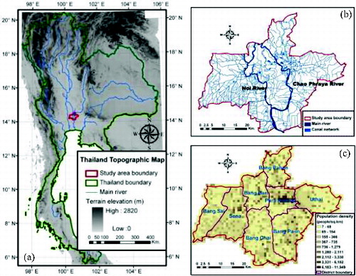
Our study area consists of eight districts in Ayutthaya: Phra Nakhon Si Ayudhya, Bang Chai, Bang Pa-in, Bang Pahan, Bang Ban, Sena, Bang Sai, and Uthai, as shown in figure 1(c). The area covers 1423.28 square kilometres with a population currently estimated at 484,439. Because the area has an extensive network of rivers and canals, as shown in figure 1(b), it is affected by flooding during the monsoon season almost every year.

Figure 1. (a) The study area located in the Chao Phraya river basin in central Thailand that was very severely affected from the 2011 Thailand major flood. (b) The river and canal network in the study area. (c) The spatial distribution of the population density in the eight districts of the study area.

2.2. Data-sets

With the advantages of synthetic aperture radar (SAR) data for water-body extraction and cloud penetration (Schumann et al. 2009), RS data used in this study is a time series of the Radarsat-2 data-set. Radarsat-2, the second in a series of Canadian spaceborne SAR satellites launched in 2007, has a single-sensor polarimetric C-band SAR (5.405 GHz) with multiple polarization modes (HH, HV, VV, and VH) and has a sun-synchronous orbit at an altitude of 798 km with a 6 PM ascending node and a 6 AM descending node. Radarsat-2 has the capability of routine left- and right-looking operation (the right-looking mode for the default operation and the left-looking mode for improved monitoring efficiencies in case of emergency imaging requests and for regions not covered in the right-looking mode, e.g. Antarctica). In this study, six Radarsat-2 scenes of 50-m resolution with the ScanSAR narrow mode were acquired on (1) 9 September 2011, (2) 3 October 2011, (3) 21 October 2011, (4) 14 November 2011, (5) 4 December 2011, and (6) 28 December 2011.

The DO values were derived from 186 flood-water samples collected by the Pollution Control Department of Thailand during the flood. The census data of each community in the study area were utilized to calculate population density, as shown in figure 1(c). The weekly surveillance reports of diarrheal patients obtained from the Bureau of Epidemiology of Thailand in Ayutthaya were employed to measure the outbreak risk and serve as the reference for the model predictions in this study.

2.3. Radarsat-2-derived flooded area

In this study, the flooded area was extracted from SAR imagery. SAR has significant advantages for the detection of water bodies and can penetrate clouds (Schumann et al. 2009). Radarsat is in operational use for flood monitoring in many countries (Brisco et al. 2008). It has been shown to accurately assess and clarify inundated areas. Moreover, its ability to penetrate clouds is very important for monitoring floods during the rainy season in monsoon countries (Hoque et al. 2011). Radarsat-2 is the second in a series of Canadian spaceborne SAR satellites that provides several improvements over Radarsat-1, such as additional beam modes, higher resolution, multi-polarization, and more-frequent revisits.

Our time series of Radarsat-2 scenes with 50-m resolution in ScanSAR narrow mode, acquired from September to December 2011, was manually orthorectified with topographic base maps, and the nearest-neighbour method was used to preserve original values in the re-sampling process. The Universal Transverse Mercator zone 47 was defined as the image-to-map projection. The acceptable threshold of the root mean square (RMS) error was set to one pixel due to limited human resources and time constraints (Rakwatin et al. 2013), and this error was considered as a buffer applied to the extraction process for areas of water bodies.

The most widely used adaptive filters based on the spatial domain to reduce the speckle noise in the SAR images include the Lee, Frost, Enfrost, Kuan, Median, and Gamma filters (Matgen et al. 2007). Using trial and error with visualization, we applied the 5 × 5 Kuan filter to reduce the speckle noise for our Radarsat-2 images (Gupta & Gupta 2007; Matgen et al. 2007). Based on the criterion of minimum mean square error, the Kuan filter applies a spatial filter to each pixel that is replaced with a value calculated based on the local statistics and can reduce speckle while preserving edges by transforming the multiplicative noise model into an additive noise model (Kuan et al. 1985; Shi & Fung 1994).

Histogram thresholding (Hostache et al. 2009) and visual interpretation (Oberstadler et al. 1997) are popular methods for delineating flooded areas based on SAR data. We therefore employed a combination of these two methods in this study (Rakwatin et al. 2013). An appropriate threshold was chosen by visual inspection of the image histogram (Matgen et al. 2007). Threshold values were manually selected for each image individually using visual interpretation to label areas as flooded or dry. To avoid misidentification due to radar backscattering from asphalt roads and permanent water bodies that may appear similar to inundated areas (Badji & Dautrebande 1997), we utilized GIS layers that included road and hydrographic features to overlay with the extracted water map (Waisurasingha et al. 2008). The output flood map was validated with ground data such as the reports of flood-relief officers and broadcast news, which were collected by the Geo-Informatics and Space Technology Development Agency (GISTDA) (Rakwatin et al. 2013) to classify each pixel as ‘flood’ or ‘non-flood’.

The resulting flooded areas in six Radarsat-2 scenes, illustrated in figure 2, show that flooding began approximately on 9 September (figure 2(a)), and continuously increased on 3 October (figure 2(b)) and 21 October (figure 2(c)) until its peak on 14 November (figure 2(d)). Subsequently, the flood gradually abated on 4 December (figure 2(e)) and 28 December (figure 2(f)). The calculated flooded area of each scene is also illustrated in figure 3(a).

Figure 2. Flooded areas delineated from a Radarsat-2 time series from September to December 2011. The inundated area continuously increased on 9 September (a), 3 October (b), and 21 October (c), peaked on 14 November (d), and gradually abated on 4 December (e) and 28 December (f).

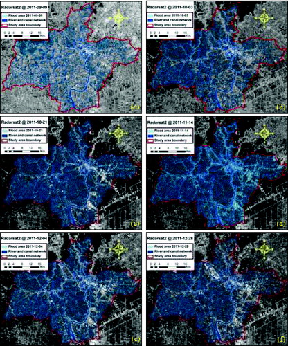
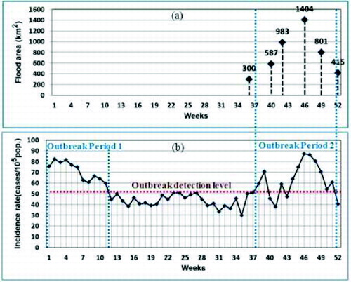
Figure 3. Relationship between flooding at various times in 2011 (a) and the weekly morbidity rate (IRR) of diarrhea with a median level of outbreak detection (b), including the two main periods of diarrheal outbreak in 2011.

2.4. Inverse distance weighting for spatial distribution

We used the inverse distance weighting (IDW) function, one of the most frequently used deterministic models in spatial interpolation (Chen & Liu 2012; Srivastava et al. 2012a; Srivastava et al. 2012b; Teegavarapu et al. 2012), to interpolate the spatial distribution of DO in the study area. IDW is relatively fast and easy to compute and straightforward to interpret. Its general concept is based on the assumption that the attribute value of an unsampled point is the weighted average of nearby known values, and the weights are inversely related to the distances between the sampled and predicted locations. Furthermore, flooding covered the entire study area at its peak. Therefore, it is plausible to consider the study area as a continuous surface and to use IDW for interpolating the spatial distribution of DO samples in the entire study area. The basic calculations for IDW (Lu & Wong 2008) are expressed in equations (1) and (2). In equation (1), IDW estimates the unknown value ŷ(S₀) in location S₀ given the observed y values at sampled locations S_i. The estimated value in S₀ is a linear combination of the weights (λ_i) and observed y values in S_i.(1) (2) In equation (2), the numerator is the inverse of the distance (d_0i) between S₀ and S_i with a power α, and the denominator is the sum of all inverse-distance weights for all locations i so that the sum of all λ_i for an unsampled point will be unity.

2.5. Measure of disease risk

The risk of contracting an illness can be expressed as the probability of infection or illness during a defined time period or may be attributed to an exposure. Analytical studies can provide a direct estimate of individual risk, and the incidence of illness among the unexposed and exposed can be directly compared. The basic measures generally used are the risk or rate difference, incidence rate ratio (IRR), cumulative incidence ratio, or odds ratio (Craun et al. 2006). To determine IRR of diarrhea due to flooding, we adapted the IRR equation from the CDC (2012) as expressed in equation (3) by defining the time period based on flood duration and letting a constant, which transforms the result of the division into a uniform quantity (n), equal 5 for fitting with the number of patients in our study. The resulting weekly IRR (cases per 10⁵ people) illustrated in figure 3(b) was calculated from the weekly report of diarrheal patients from hospitals in the study area.(3) In comparing the rates of disease of two groups, the relative risk, or risk ratio (RR), is widely used to compare the disease rates that differ by demographic characteristics or exposure histories as shown in equation (4) (Craun et al. 2006; CDC 2012). In this study, RR was employed to define the risk of diarrheal outbreak due to flooding by comparing the IRR of diarrhea during floods with the median IRR of diarrhea in the study area in 2011.(4)

2.6. BPNN

Artificial neural networks (ANNs) are an important class of tools for quantitative modelling. One of the powerful characteristics of ANNs is the ability to learn relationships between inputs and outputs via training (Bai & Jin 2005). After the training process, the neural network can give correct answers not only for learned examples, but also for inputs similar to the learned examples. The ANN approach is suitable for solving large, non-linear, and complex problems of classification and functional approximation (Srivastava et al. 2013). BPNN, i.e. MLP with back propagation, is the most popular type of ANN (Han & Kamber 2006; Lee & Hsiung 2009). BPNN has been used to assess uncertainties in epidemics or disasters in many studies (Kanevski et al. 2004; Bai & Jin 2005; Cao et al. 2010a).

The MLP configuration consists of three basic layers of interconnected neurons (input layer, hidden layers, and output layer). Each connection has a weight associated with it, as illustrated in figure 4.

Figure 4. The typical structure of BPNN including the three basic layers (input, hidden, and output layers) and the two main steps (input feed-forward network and back propagation) adapted from Lee and Hsiung (2009) and Han and Kamber (2006).

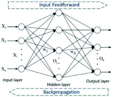
BPNN or MLP with the back propagation approach has two main steps: input feed forward, i.e. multi-layer feed-forward network (Witten & Frank 2005; Maimon & Rokach 2010), and back propagation. The input units are fed by the relational database (a collection of tables). Each table consists of a set of attributes (columns or fields) and usually stores a large set of tuples (records or rows). Each tuple in a relational table represents an object identified by a unique key and described by a set of attribute values. Each training example consists of a tuple of values, one value for each input dimension in the problem. During training, the tuples are fed into the network, along with the correct outputs (target values). To propagate the inputs forward, the training tuple is fed to the input layer of the network, one value per neuron in the input layer. For each tuple X_i, the network modifies weights to values that minimize the mean square error between the network prediction and the actual target value. The net input to a unit in the hidden or output layers is computed as a linear combination of its inputs. To compute the net input to the unit, each input connected to the unit in the next layer is multiplied by its corresponding weight and is then summed. Given a unit j in a hidden or output layer, the net input, I_j, to unit j can be expressed in equation (5) (Han & Kamber 2006).(5) where w_ij is the weight of the connection from unit i in the previous layer to unit j, O_i is the output of unit i from the previous layer, and θ_j is the bias of the unit.

In the back-propagation step, the error is propagated backward by updating the weights and biases to reflect the error of the network prediction. To compute the error of a hidden layer unit j, the weighted sum of the errors of the units connected to unit j in the next layer is considered. The error of a hidden layer unit j is shown in equation (6) (Han & Kamber 2006).(6) where O_j is the actual output of unit j, w_jk is the weight of the connection from unit j to a unit k in the next higher layer, and Err_k is the error of unit k.

In this study, we used measures of flood duration, DO, and population density at various locations as the input dimensions, and they were normalized to lie in a fixed range, from zero to one, by subtracting the minimum value and dividing by the range between the maximum and the minimum values (Witten & Frank 2005). With the best spatial resolution of our input parameters, which were the 50-m Radarsat-2 data, each tuple fed into the network was defined as each centre point of a 50-m grid (point-based), and each value for each input dimension was determined by the pixel value of flood duration, DO, and population-density map in which its tuple fell. We used the RR of outbreak based on surveillance reports as reference data for training. After the model was trained, we used it to predict RR for a new set of tuples.

3. Results and discussion

3.1. Flood duration

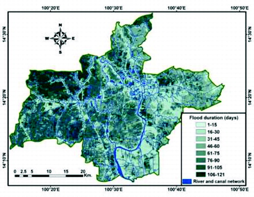
We obtained the flood duration in each area by comparing the maps of the flooded areas, which were derived from the six multi-temporal Radarsat-2 scenes. The flood-duration map in figure 5 shows that the inundated area covered the entire study area at its peak. The longest inundated period was over 4 months, while the shortest was barely 1 week. As a first priority, the Thai government and private sectors aimed to prevent or reduce the water level in urban areas, along transportation routes and in residential and industrial areas, by draining flood water into agricultural areas, particularly rice fields, which are frequently located in low-lying areas. Therefore, the areas with the longest flood durations tend to be agricultural areas.

Figure 5. Flood duration estimated from a time series of Radarsat-2 scenes.

3.2. Spatial distribution of DO

In a flood disaster, faecal coliform bacteria or E. coli are common causes of diarrhea because the flooding washes faecal material from human habitats, causing increased transmission of bacterial infection. To investigate waterborne disease, almost all studies have attempted to determine the presence of pathogens such as bacteria and viruses in contaminated water based on QMRA. Time-consuming laboratory testing is required to determine the amount of pathogens in each water sample.

DO is an important indicator of river health (the ecological condition of a river) and is used by regulators as part of the classification scheme for good chemical status (Williams & Boorman 2012). Therefore, researchers have frequently used DO to evaluate water quality (Kannel et al. 2007). In addition, DO has a close relationship to faecal coliform bacteria. Because these bacteria are oxidase negative, if DO decreases, coliform bacteria frequently increase, and vice versa. In this study, DO was used as an input factor governing the risk of diarrheal infection of people in inundated areas. We obtained 186 DO samples from the Pollution Control Department of Thailand, which were taken during flooding, as shown in figure 6.

Figure 6. The spatial distribution of dissolved oxygen (DO) estimated from 186 flood-water samples based on inverse distance weighting (IDW).

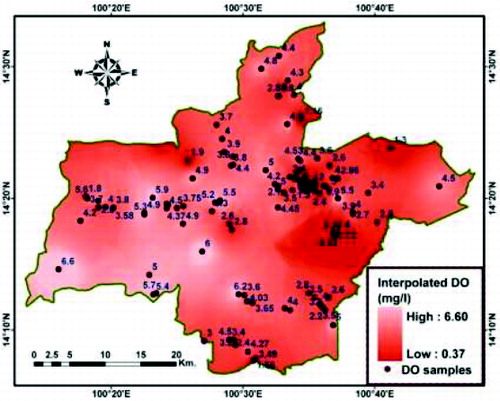
As discussed above, we used IDW to interpolate these point measures into a continuous grid. The resulting map after interpolation, shown in figure 6, illustrates the DO spatial distribution. Higher DO values indicate better water quality. Thus, the redder areas in figure 6 have poorer water quality. Overlaying the water-quality map on a land-use layer, we found that the intensely red area on the bottom right of figure 6 is the location of major industrial estates in Bang Pa-in. The faecal and chemical materials leaking from industrial factories caused a very low value of DO in this area. The best water quality, with the highest values of DO, was mostly located in the countryside or in agricultural areas. The mean value of DO of each district is given in table 1.

Table 1. The risk ratio (RR) of diarrheal outbreak due to flooding and the related parameters for the eight districts in the study area.

District	Population	Area (km^2)	Population density (people/km^2)	Mean flood duration (days)	Mean DO (mg/l)	Diarrheal morbidity	Risk ratio
Sena	66,122	215.28	307.14	67	3.6	716	1.48
Bang Ban	34,379	136.75	251.40	53	3.9	183	1.45
Uthai	46,540	170.62	272.77	40	3.3	462	1.32
Bang Sai	19,685	164.72	119.51	75	4.3	138	1.23
Bang Pa-in	90,188	237.10	380.38	35	3.0	711	1.15
Phra Nakhon Si Ayudhya	139,129	117.82	1180.86	30	3.6	1651	1.14
Bang Chai	47,083	250.03	188.31	44	3.9	292	0.99
Bang Pahan	41,313	130.96	315.46	44	3.7	195	0.82

The RMS cross-validation error (Joseph & Kang 2011), which is an assessment of the uncertainty of the IDW interpolation of the DO spatial distribution, is 0.078 mg/l, while the resolutions of the DO meters or the average standard errors of our DO measurements range from 0.01 to 0.10 mg/l. The similarity between the interpolation error and the measurement error indicates that we are correctly assessing the variability in the interpolation.

3.3. Detection of diarrheal outbreak

In this study, we want to detect outbreaks of diarrhea. However, there is no generally accepted number or percentage increase of cases that defines an outbreak or epidemic (Craun et al. 2006). What public health officials consider is usually based on previous surveillance, with an outbreak identified when the number of cases is greater than expected for a specific disease or set of symptoms in that area. The IRR of an outbreak period is expected to be higher than that for other periods in the same area. For this study, we set the definition of diarrheal outbreak (Schwartz et al. 2006) after plotting the relationship between the weekly flooded area as derived from RS and the weekly IRR, as shown in figure 3(a) and 3(b), respectively. We defined the onset of an outbreak during weeks 38–51 in 2011, when the weekly diarrheal morbidity exceeded the 2011 median for a district or exceeded 50.37 cases per 100,000 population for the entire study area.

From figure 3(b), we found that the study area had two main periods of diarrheal outbreaks in 2011, during weeks 1–11 and 38–51. After interviewing the officers of the Ministry of Public Health in Ayutthaya province, we found that the first period at the beginning of the year was probably a result of the long celebrations during the New Year festival, from frequent alcohol consumption or ingestion of unhygienic food. Therefore, we concentrated on the second outbreak occurring during the flood. A comparison of figure 3(a) and 3(b) demonstrated that there was a very close relationship between the flooded area and outbreak intensity. Flooding started, peaked, and abated in weeks 36, 46, and 52, respectively, and the second outbreak period started in week 38. Although the IRR values in weeks 39, 40, and 43 were lower than the outbreak detection level, it peaked in week 46 and, like the water, also abated in week 52.

To estimate the risk of diarrheal outbreak due to flooding for each district, the RR was used to compare the IRR of weekly morbidity with the outbreak detection level or the median of weekly morbidity. An RR less than or equal to 1 indicates no outbreak or no risk. Otherwise, it indicates the possibility of an outbreak, with outbreak intensity increasing with larger values of RR (Craun et al. 2006).

Table 1 shows the RR of each district during weeks 36–52, derived from the diarrheal morbidity reported by hospitals, with the means of three main parameters: population density, flood duration, and DO. Theoretically, an area having high population density, long flood duration, or lower DO should have a high risk of disease and vice versa. The mean values of each district in table 1 suggest that all three parameters affect the risk of diarrheal outbreak. For example, although the Bang Pa-in and Phra Nakhon Si Ayudhya districts had the worst DO quality and the highest population density, respectively, their outbreak risks were moderate due to the comparatively short duration of their floods. Even though the Bang Sai district had the longest flood duration, its outbreak risk was also moderate due to having the lowest population density.

3.4. Modelling of diarrheal-outbreak risk due to flooding

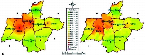
In this study, we aim to model the outbreak risk of diarrhea due to flooding by using the BPNN approach. The RR of each district in table 1 was spatially spread over the study area based on IDW to produce the target values for BPNN training and testing. We defined the RR position as the location of the hospital in each district, because in general diarrheal patients should go to the district hospital nearest to their habitations. Thus, it is plausible to employ IDW to spatially interpolate the outbreak risk by considering the distance from the training/testing point to the district hospital. In addition, we also added some RRs of district hospitals outside the study area for better interpolation near the boundaries of the study area. The reference risk map and the locations of district hospitals are shown in figure 7(a).

Figure 7. Comparison of the reference risk map derived from the diarrheal-morbidity rate at hospitals in the study area during flooding (left) and the risk map of diarrheal outbreak simulated by the BPNN prediction model (right); a risk ratio (RR) less than or equal to 1 indicates no outbreak or no risk, otherwise the possibility of an outbreak or the outbreak intensity increases with RR.

The map resolution was defined by the best spatial resolution of our input parameters, which was the 50 m × 50 m resolution of the Radarsat-2 data. We had a total of 569 × 122 points (pixels). These points were divided into two groups: 66% for training and 34% for testing, which is the default setting for splitting learning data in WEKA (Bouckaert et al. 2012), a popular open-source machine-learning software developed by the University of Waikato, New Zealand.

In the training process, setting a suitable number of neurons in the hidden layer is very important. If the number of hidden neurons exceeds an appropriate value, the computation is time-consuming and unstable. On the other hand, if the number of neurons is too small, the training process may not converge (Cao et al. 2010a). Due to the large number of data tuples, we decided to split the input data by district. The numbers of hidden-layer neurons for each district, which ranged from 3 to 9, are shown in table 2.

Table 2. The number of inputs for training and testing, the appropriate number of hidden layers, and the correlation coefficients and RMS errors of the BPNN model prediction computed using WEKA (open-source software).

District	Trained inputs	Tested inputs	Hidden layers	Correlation coefficient	RMS error
Sena	56,998	29,096	3	0.81	0.065
Bang Ban	36,036	18,662	8	0.83	0.038
Uthai	44,891	23,362	8	0.81	0.037
Bang Sai	43,371	22,501	5	0.93	0.035
Bang Pa-in	62,770	32,086	9	0.83	0.014
Phra Nakhon Si Ayudhya	31,105	16,014	7	0.79	0.029
Bang Chai	66,051	33,953	4	0.83	0.048
Bang Pahan	34,398	17,828	7	0.88	0.060

To evaluate the prediction success, we assessed the accuracy by using correlation coefficients (R-values) and RMS errors. RMS error is the most commonly used measure in mathematical techniques to assess how close the predicted values from the model are to the actual or reference values, while the correlation coefficient can measure the statistical relationship between the test instances and the actual or reference values and indicate how well the data points or instances fit the linear line (Witten & Frank 2005). The results of our BPNN predictions in table 2 show that the correlation coefficients range from 0.79 to 0.93 (the correlation coefficient ranges from 1, for perfectly correlated results, to 0, when there is no correlation, to −1 when the results are perfectly correlated negatively), RMS errors range from 0.014 to 0.065, and the predicted RRs range from 0.82 to 1.57. The high correlation coefficients indicate that our results have a very good correlation with the reference or actual data, and the low RMS errors indicates that the predicted RR from the model and the reference RR derived from the morbidity data are close to each other. An RR resolution (the difference of two RR values) below 0.1 indicates an indifferent risk for classifying the strength of an epidemiological association (Craun et al. 2006). This can imply that the range of our RMS errors is less than the adequate RR resolution to classify the level of outbreak risk. As discussed above, we can conclude that our predictive model for each district can give accurate predictions.

Finally, we created a map of the risk of diarrheal outbreak as predicted by the BPNN model, as shown in figure 7(b). Comparing the predicted risk map with the reference risk map derived from the morbidity rates at the hospitals in figure 7(a), we can see that the simulated risk map reflects the actual risk and trends. For example, both maps show high risk in Bang Ban and Sena, no or low risk in Bang Chai and Bang Pa-in, and moderate risk in Bang Sai, Phra Nakhon Si Ayudhya, and Uthai. With the high spatial resolution of the resulting map, decision-makers can use the map as an effective tool to protect communities and mitigate the effects of diarrheal disease due to flooding.

Compared with other common approaches that also aim to estimate the risk of waterborne disease, our approach has the advantage of requiring only simple input data, in particular water-sampling data. Instead of using other parameters of water quality, such as E. coli and faecal coliform concentrations that need complicated and time-consuming laboratory testing, our approach utilizes DO, which can easily and instantly be measured by DO meters. In addition, DO is widely used as an indicator of water quality of the water-quality surveillance system in many countries, therefore DO data will be frequently updated from the measurement stations. In Thailand, for instance, DO values are measured roughly once a week. Thus our approach can better model the outbreak risk in near real time with up-to-date input data. The predicted risk can also help the decision-maker to prioritize outbreak prevention and response when flooding occurs so that the appropriate measures can be taken.

4. Conclusions

Waterborne infectious diseases, particularly diarrhea, are a serious problem when floods occur. Dirty flood water contaminated with pathogenic microorganisms is a key factor causing people to become infected. To prevent waterborne outbreaks, numerous studies have attempted to detect and assess the risk of waterborne diseases based on the direct measurement of pathogens, but the complicated and time-consuming laboratory testing cause a lack of samples for comprehensively modelling and analysing the risk in flood-affected areas. In contrast, based on the BPNN technique, this study provided an approach to assess the outbreak risk of diarrhea due to flooding by using simple parameters, including flood duration, DO, and population density. A time series of Radarsat-2 scenes were utilized to spatially define flood duration, which in 2011 ranged from a week to 4 months. Samples of DO content were used to estimate the spatial distribution of flood-water quality in inundated areas. The data showed that the poorest quality of flood water appeared in major industrial estates and some rural areas, while a better quality of flood water was mostly located in the countryside or in agricultural areas. We used the RR function on data from weekly surveillance reports of the diarrheal morbidity from district hospitals in the study area for detection of the diarrheal outbreaks due to the flood. The mean RRs of eight districts of Ayutthaya province in the study area were between 0.82 and 1.48. (An RR less than or equal to 1 indicates no outbreak or no risk. Otherwise it indicates the possibility of an outbreak, with outbreak intensity increasing with larger values of RR.) The BPNN model produced very good prediction accuracy, with high correlation coefficients, which measure the statistical correlation between predicted and reference RR, ranging from 0.79 to 0.93 (the correlation coefficient ranges from 1 for perfectly correlated results to 0 when there is no correlation), and acceptable RMS errors, ranging from 0.014 to 0.065. This indicates that the predictive models of the diarrheal-outbreak risk for each district are very accurate.

We can thus conclude that our approach is a promising method for modelling the risk of diarrheal outbreak in a flood disaster and will be useful for making decisions regarding preventive measures and countermeasures by spatial analysis. Compared with other common approaches using pathogen parameters, our approach has the advantage of only requiring simple input data, leading to rapidly and comprehensively assessing the outbreak risk in floods. Embedding this approach into the near real-time flood-monitoring system organized by GISTDA (http://flood.gistda.or.th), to prevent future outbreaks due to floods in Thailand, can assist public-health and relief agencies to prioritize aid, public-health action, and temporary evacuation centres for people affected by flood disasters.

For further work, other factors affecting epidemics in a flood situation, such as emigration, the conditions of hygiene in various localities, and the flood intensity, can be added to the model. Theoretically, adding more impact factors should produce better results, but on the other hand, this also requires more effort, cost, and time. The advantages and disadvantages must be weighed. It may also be useful to apply this approach to other waterborne infectious diseases.

Acknowledgements

This study was supported by the Twentieth Session of Joint Committee on Scientific and Technical Cooperation between the Government of China and Thailand (grant no. 20-624J) and the Wetland Ecosystem Assessment program of the State Forestry Administration of China. The authors gratefully acknowledge the Pollution Control Department of Thailand and the Research and Laboratory Development Center of Department of Health of Thailand for providing water-sample data, Geo-Informatics and Space Technology Development Agency (GISTDA) for providing the flood-area data-set, and the Bureau of Epidemiology of Thailand in Ayutthaya province for providing the weekly surveillance reports of diarrheal patients.

References

- Badji M, Dautrebande S. 1997. Characterization of flood inundated areas and delineation of poor drainage soil using ERS-1 SAR imagery. Hydrological Processes. 11:1441–1450.
- Bai YP, Jin Z. 2005. Prediction of SARS epidemic by BP neural networks with online prediction strategy. Chaos Solitons Fractals. 26:559–569.
- Boonsoong B, Sangpradub N, Barbour MT, Simachaya W. 2010. An implementation plan for using biological indicators to improve assessment of water quality in Thailand. Environ Monit Assess. 165:205–215.
- Bouckaert RR, Frank E, Hall M, Kirkby R, Reutemann P, Seewald A, Scuse D. 2012. WEKA manual for version 3.7.6. Hamilton, New Zealand: University of Waikato.
- Brisco B, Touzi R, van der Sanden JJ, Charbonneau F, Pultz TJ, D’Iorio M. 2008. Water resource applications with RADARSAT-2-a preview. Int J Digital Earth. 1:130–147.
- Cao CX, Chang CY, Xu M, Zhao JA, Gao MX, Zhang H, Guo JP, Guo JH, Dong L, He QS, et al. 2010a. Epidemic risk analysis after the Wenchuan earthquake using remote sensing. Int J Remote Sensing. 31:3631–3642.
- Cao CX, Xu M, Chang CY, Xue Y, Zhong SB, Fang LQ, Cao WC, Zhang H, Gao MX, He QS, et al. 2010b. Risk analysis for the highly pathogenic avian influenza in Mainland China using meta-modelling. Chin Sci Bull. 55:4168–4178.
- Cao CX, Xu M, Chen W, Tian R. 2012. A framework for diagnosis of environmental health based on remote sensing. Land Surf Remote Sensing. 8524:852414.
- [CDC] Centers for Disease Control and Prevention. 2012. Principles of epidemiology in public health practice: an introduction to applied epidemiology and biostatistics. CDC. Available from: http://www.cdc.gov/osels/scientific_edu/ss1978/SS1978.pdf
- Chang LC, Shen HY, Wang YF, Huang JY, Lin YT. 2010. Clustering-based hybrid inundation model for forecasting flood inundation depths. J Hydrology. 385:257–268.
- Chen FW, Liu CW. 2012. Estimation of the spatial rainfall distribution using inverse distance weighting (IDW) in the middle of Taiwan. Paddy Water Environ. 10:209–222.
- Constantin de Magny G, Murtugudde R, Sapiano MRP, Nizam A, Brown CW, Busalacchi AJ, Yunus M, Nair GB, Gil AI, Lanata CF, et al. 2008. Environmental signatures associated with cholera epidemics. Proc Natl Acad Sci USA. 105:17676–17681.
- Craun GF, Calderon RL, Wade TJ. 2006. Assessing waterborne risks: an introduction. J Water Health. 4(Suppl 2):3–18.
- Ford TE, Colwell RR, Rose JB, Morse SS, Rogers DJ, Yates TL. 2009. Using satellite images of environmental changes to predict infectious disease outbreaks. Emerging Infect Dis. 15:1341–1346.
- Gupta KK, Gupta R. 2007. Despeckle and geographical feature extraction in SAR images by wavelet transform. Isprs J Photogrammetry Remote Sensing. 62:473–484.
- Han J, Kamber M. 2006. Data mining: concepts and techniques. San Francisco: Elsevier.
- Herbreteau V, Salem G, Souris M, Hugot J-P, Gonzalez J-P. 2007. Thirty years of use and improvement of remote sensing, applied to epidemiology: from early promises to lasting frustration. Health Place. 13:400–403.
- Hoque R, Nakayama D, Matsuyama H, Matsumoto J. 2011. Flood monitoring, mapping and assessing capabilities using RADARSAT remote sensing, GIS and ground data for Bangladesh. Nat Hazards. 57:525–548.
- Hostache R, Matgen P, Schumann G, Puech C, Hoffmann L, Pfister L. 2009. Water level estimation and reduction of hydraulic model calibration uncertainties using satellite SAR images of floods. IEEE Trans Geosci Remote Sensing. 47:431–441.
- Howard G, Pedley S, Tibatemwa S. 2006. Quantitative microbial risk assessment to estimate health risks attributable to water supply: can the technique be applied in developing countries with limited data? J Water Health. 4:49–65.
- Islam MS, Brooks A, Kabir MS, Jahid IK, Islam MS, Goswami D, Nair GB, Larson C, Yukiko W, Luby S. 2007. Faecal contamination of drinking water sources of Dhaka city during the 2004 flood in Bangladesh and use of disinfectants for water treatment. J Appl Microbiol. 103:80–87.
- Joseph VR, Kang LL. 2011. Regression-based inverse distance weighting with applications to computer experiments. Technometrics. 53:254–265.
- Kanevski M, Parkin R, Pozdnukhov A, Timonin V, Maignan M, Demyanov V, Canu S. 2004. Environmental data mining and modeling based on machine learning algorithms and geostatistics. Environ Modelling Software. 19:845–855.
- Kannel PR, Lee S, Lee YS, Kanel SR, Khan SP. 2007. Application of water quality indices and dissolved oxygen as indicators for river water classification and urban impact assessment. Environ Monit Assess. 132:93–110.
- Kazama S, Aizawa T, Watanabe T, Ranjan P, Gunawardhana L, Amano A. 2012. A quantitative risk assessment of waterborne infectious disease in the inundation area of a tropical monsoon region. Sustainability Sci. 7:45–54.
- Kersters I, Vanvooren L, Huys G, Janssen P, Kersters K, Verstraete W. 1995. Influence of temperature and process technology on the occurrence of aeromonas species and hygienic indicator organisms in drinking-water production plants. Microb Ecol. 30:203–218.
- Kuan DT, Sawchuk AA, Strand TC, Chavel P. 1985. Adaptive noise smoothing filter for images with signal-dependent noise. IEEE Trans Pattern Anal Machine Intelligence. 7:165–177.
- Lee CJ, Hsiung TK. 2009. Sensitivity analysis on a multilayer perceptron model for recognizing liquefaction cases. Comput Geotechnics. 36:1157–1163.
- Lleo MD. 2009. Application of space technologies to the surveillance and modelling of waterborne diseases. Trop Med Int Health. 14:23–23.
- Lu GY, Wong DW. 2008. An adaptive inverse-distance weighting spatial interpolation technique. Comput Geosci. 34:1044–1055.
- Maimon O, Rokach L. 2010. Data mining and knowledge discovery handbook. New York (NY): Springer.
- Massoud MA. 2012. Assessment of water quality along a recreational section of the Damour River in Lebanon using the water quality index. Environ Monit Assess. 184:4151–4160.
- Matgen P, Schumann G, Henry JB, Hoffmann L, Pfister L. 2007. Integration of SAR-derived river inundation areas, high-precision topographic data and a river flow model toward near real-time flood management. Int J Appl Earth Observation Geoinformation. 9:247–263.
- Oberstadler R, Honsch H, Huth D. 1997. Assessment of the mapping capabilities of ERS-1 SAR data for flood mapping: a case study in Germany. Hydrological Processes. 11:1415–1425.
- Osode AN, Okoh AI. 2010. Survival of free-living and plankton-associated Escherichia coli in the final effluents of a waste water treatment facility in a peri-urban community of the Eastern Cape Province of South Africa. Afr J Microbiol Res. 4:1424–1432.
- Rakwatin P, Sansena T, Marjang N, Rungsipanich A. 2013. Using multi-temporal remote-sensing data to estimate 2011 flood area and volume over Chao Phraya River basin, Thailand. Remote Sensing Lett. 4:243–250.
- Schumann G, Bates PD, Horritt MS, Matgen P, Pappenberger F. 2009. Progress in integration of remote sensing-derived flood extent and stage data and hydraulic models. Rev Geophys. 47:RG4001.
- Schwartz BS, Harris JB, Khan AI, Larocque RC, Sack DA, Malek MA, Faruque ASG, Qadri F, Calderwood SB, Luby SP, Ryan ET. 2006. Diarrheal epidemics in Dhaka, Bangladesh, during three consecutive floods: 1988, 1998, and 2004. Am J Trop Med Hyg. 74:1067–1073.
- Shi ZG, Fung KB. 1994. A Comparison of digital speckle filters. 1994 International Geoscience and Remote Sensing Symposium (IGARSS), pp. 2129–2133.
- Srivastava P, Gupta M, Mukherjee S. 2012a. Mapping spatial distribution of pollutants in groundwater of a tropical area of India using remote sensing and GIS. Appl Geomatics. 4:21–32.
- Srivastava PK, Han DW, Gupta M, Mukherjee S. 2012b. Integrated framework for monitoring groundwater pollution using a geographical information system and multivariate analysis. Hydrological Sci J. 57:1453–1472.
- Srivastava PK, Han DW, Ramirez MR, Islam T. 2013. Machine learning techniques for downscaling SMOS satellite soil moisture using MODIS land surface temperature for hydrological application. Water Resour Manag. 27:3127–3144.
- Teegavarapu RSV, Meskele T, Pathak CS. 2012. Geo-spatial grid-based transformations of precipitation estimates using spatial interpolation methods. Comput Geosci. 40:28–39.
- Tran A, Goutard F, Chamaille L, Baghdadi N, Lo Seen D. 2010. Remote sensing and avian influenza: a review of image processing methods for extracting key variables affecting avian influenza virus survival in water from earth observation satellites. Int J Appl Earth Observation Geoinformation. 12:1–8.
- Waisurasingha C, Aniya M, Hirano A, Sommut W. 2008. Use of RADARSAT-1 data and a digital elevation model to assess flood damage and improve rice production in the lower part of the Chi River Basin, Thailand. Int J Remote Sensing. 29:5837–5850.
- Williams RJ, Boorman DB. 2012. Modelling in-stream temperature and dissolved oxygen at sub-daily time steps: an application to the River Kennet, UK. Sci Total Environ. 423:104–110.
- Witten IH, Frank E. 2005. Data mining: practical machine learning tools and techniques. San Francisco: Elsevier.
- Yomwan P, Cao CX, Rakwatin P, Apaphant P. 2012. The risk analysis for infectious disease outbreaks in flood disaster based on spatial information technologies. 2012 IEEE International Geoscience and Remote Sensing Symposium (IGARSS), pp. 7244–7247.