Glacial lake outburst flood risk assessment using combined approaches of remote sensing, GIS and dam break modelling

Abstract

A great number of glacial lakes have appeared in many mountain regions across the world during the last half-century due to receding of glaciers and global warming. In the present study, glacial lake outburst flood (GLOF) risk assessment has been carried out in the Teesta river basin located in the Sikkim state of India. First, the study focuses on accurate mapping of the glaciers and glacial lakes using multispectral satellite images of Landsat and Indian Remote Sensing satellites. For glacier mapping, normalized difference snow index (NDSI) image and slope map of the area have been utilized. NDSI approach can identify glaciers covered with clean snow but debris-covered glaciers cannot be mapped using NDSI method alone. For the present study, slope map has been utilized along with the NDSI approach to delineate glaciers manually. Glacial lakes have been mapped by supervised maximum likelihood classification and normalized difference water index followed by manual editing afterwards using Google Earth images. Second, the first proper inventory of glacial lakes for Teesta basin has been compiled containing information of 143 glacial lakes. Third, analysis of these lakes has been carried out for identification of potentially dangerous lakes. Vulnerable lakes have been identified on the basis of parameters like surface area, position with respect to parent glacier, growth since 2009, slope, distance from the outlet of the basin, presence of supraglacial lakes, presence of other lakes in downstream, condition of moraine, condition of the terrain around them, etc. From these criterions, in total, 18 lakes have been identified as potentially dangerous glacial lakes. Out of these 18 lakes, further analysis has been carried out for the identification of the most vulnerable lake. Lake 140 comes out to be the most vulnerable for a GLOF event. Lastly, for this potentially dangerous lake, different dam break parameters have been generated using satellite data and digital elevation model. The volume and depth have been computed using empirical formulae, and other parameters such as cross-sections from the lake to outlet etc. have been prepared in ArcGIS 9.3. The GLOF which can be triggered by Lake 140 was modelled and simulated using MIKE-11 software's hydrodynamic module. As a result, flood values and hydrograph have been obtained. The flood at lake site comes out to be 2611.136 cumec which get mitigated to 1417.844 cumec at the outlet.

1. Introduction

Many glaciers all over the globe are receding. Inventory of glaciers and glacial lakes prepared by ICIMOD (International Centre for Integrated Mountain Development) for Himalayan region shows that glacial lakes are increasing in number and volume due to thinning and recession of glaciers (Mool et al. 2001) Receding glaciers give rise to glacial lakes when melt water gets accumulated behind semi-permanent structures like moraines and ice. Bursting of these lakes by sudden breach in moraine or ice can cause flash flood in the downstream areas (Watanabe et al. 1994). These glacial lake outburst floods (GLOFs) are capable of causing great damage to human lives and property; therefore, monitoring the health of these lakes is necessary. Due to their remote locations and high altitude, monitoring of these lakes is a very difficult task by traditional surveys (Mool 1995). Remote sensing offers a useful tool for monitoring these lakes as most of the parameters related to glacial lakes can be studied using remote sensing (Bloch 2008). Key factors contributing to glacial lake hazard and its monitoring, using remote sensing, are lake volume and rate of formation, reaction of glacier to climate, activity of glacier, possibility of mass moments into lake, stability, width and height of moraine, and situation down valley (Richardson & Reynolds 2000; Quincey et al. 2005). Several studies have shown the potential of remote sensing in monitoring glacial lakes and preparing their inventory all over the globe from Alps (Huggel et al. 2002; Paul & Andreassen 2009) to the Himalayas (Quincey & Richardson 2007). For mapping glacial lakes, thresholding of normalized difference water index (NDWI) image is most popular, but owing to mountain shadows, ice cover and turbidity of water manual checking is always necessary.

Mapping of glaciers is an important part of the glacial lake hazard assessment as their position with respect to lakes, their slope and surface area play an important part in assessing glacial lake hazard. Remote sensing is, in general, the only possible method for mapping and monitoring these glaciers. Much of the work has been carried out to analyse glacier and glacier changes using remote sensing. Several supervised classification, unsupervised classification and ratio methods are available for glacier mapping, but thresholding of normalized difference snow index (NDSI) image and time-intensive manual delineation is generally known to be most accurate (Paul 2000). NDSI is generally used for snow cover mapping using satellite data (Hall et al. 1995; Kulkarni et al. 2001; Kulkarni & Bahuguna 2009). NDSI uses high and low reflectance of snow in visible (green) and short-wave infrared region, respectively, and it can also delineate and map snow in mountain shadows (Kulkarni et al. 2001). Equation (1(1) ) shows the formula of NDSI. (1)

Clean ice glaciers can be mapped using NDSI but many glaciers in the Himalayas are characteristically debris covered. Manual delineation is, in general, still possible because the glacier boundary exhibits differences in illumination caused by its shape. Morphometric parameters derived from digital elevation model (DEM), such as slope, have shown potential for mapping debris-covered glaciers.

Modelling of GLOF is akin to the dam break study of the moraine dams, which assesses the flood hydrograph of the discharge from the dam breach and discharge time series at different locations of the river downstream of the dam due to propagation of flood waves. Dam break flood simulation studies can be carried out by either scaled physical hydraulic models or mathematical simulation models. Several models such as DAMBRK, BREACH, SOBEK, etc. have been used in past studies to carry out GLOF simulations (WECS 1987; Carrivick 2006; Bajracharya et al. 2007). The mathematical models which approximately solve the governing flow equations of continuity and momentum by computer simulation are the cost-effective modern tools for the dam break analysis. The essence of dam break modelling is hydrodynamic modelling, which involves finding solution to partial differential equations (equations (2) and (3)) which are known as Saint-Venant equations (Saint-Venant 1871). (2) (3) where Q = discharge, A = active flow area, A₀ = inactive storage area, h = water surface elevation, q = lateral flow, X = distance along waterway, t = time, S_f = friction slope, S_c = expansion contraction slope and g = gravitational acceleration.

MIKE-11 is a professional software package for supporting dam break modelling by solving above equations in its HD module. It has been used successfully for GLOF simulation (Sharma et al. 2009). Simulation of dam breach requires several inputs and parameters which fall in three categories:

1. lake information (volume, area and depth);

2. dam breach parameters (breach invert level, time of formation of breach, breach width);

3. cross-sections from lake to the outlet of the basin, these are used to model the channel's topography and routing the water.

While area can be computed easily after mapping the lake, direct computation of volume and depth computation is not possible. However, empirical relations exist, relating area with depth and volume. Dam break parameters are obtained using Froelich's dam breach prediction equations. Cross-sections are prepared from DEM using geographical information system (GIS) tools.

2. Study area and data used

2.1. Study area

The study area taken in this study is the Teesta basin (figure 1). Entire Indian state of Sikkim constitutes the basin of river Teesta. Sikkim is a small Himalayan state in north-east India situated between 27° 00′ 46″ to 28° 07′ 48″ N latitude and 88° 00′ 58″ to 88° 55′ 25″ E longitude with a geographical area of 7096 km². The state is somewhat rectangular in shape with a maximum length from north to south of about 112 km and the maximum width from east to west of 90 km. Sikkim state, being a part of inner mountain ranges of the Himalayas, is entirely hilly, having no plain area with altitude varying from 213 m in the south to above 8000 m in the north-west and north. Teesta basin is endowed with number of glacial lakes of various sizes and shapes. More than 43% of Teesta basin in Sikkim is characterized by very steep slopes and escarpments, i.e. more than 43% of its geographical area lies in more than 50% slope category.

Figure 1. Study area.

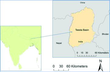
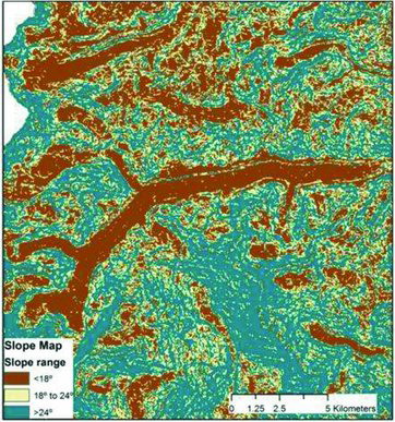
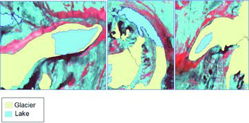
Figure 2. Classification of slope at Zemu glacier region, Sikkim, Indian Himalayas.

2.2. Data used

In the present study, satellite scenes of IRS-LISS III and Landsat have been used. For topographic information, ASTER GDEM (global DEM) has been utilized. The GDEM was created by stereo-correlating the 1.3 million scenes of ASTERVNIR archive, covering the Earth's land surface between 83N and 83S latitudes. The GDEM is produced with 30-m postings and is formatted in 1 × 1 degree tiles as GeoTIFFfiles. The GDEM is referenced to the WGS84/EGM96 geoid. The GDEM's vertical accuracy is 7–14 m (source: http://www.jspacesystems.or.jp/ersdac/GDEM/E/2.html). GDEM has been used successfully in the Himalayas for hydrodynamic modelling (Jain et al. 2012). GDEM can be used successfully in generating river centre lines, cross-sections, etc. for hydrodynamic modelling of GLOF in the Himalayan regions with tolerable errors (Wang et al. 2012). Google Earth images were also used for carrying out manual checking and analysis. The specification of the data used is given in table 1.

Table 1. Data used.

Sensor/source	Product	Date	Resolution
IRS, LISS-3	Satellite image	27 October 2011	23.5 m
LANDSAT, TM	Satellite image	20 July 2009	30 m
TERRA, ASTER	GDEM	–	30 m
Google Earth images	Satellite images	21 December 2011

3. Methodology

The methodology used for glacial lake hazard monitoring can be summed up in six phases.

3.1. Database generation

In the first step, preprocessing of satellite data has been carried out, Landsat and Indian Remote Sensing (IRS) images were geometrically corrected; however, no atmospheric correction was applied owing to clear weather during those days. IRS image has been re-sampled to 30 m using nearest neighbourhood method in order to match the spatial resolution of Landsat image, and both the images from Landsat and IRS were calibrated to convert digital values to true reflectance. Topographically corrected reflectance values have been obtained using C-correction method (Teillet et al. 1982). Slope, elevation and drainage maps were prepared which were required for analysis in later stages.

3.2. Glacier mapping

In the present study, for mapping of snow-covered glacier, NDSI approach has been used. As given by Paul et al. (2004), use of slope can be used for debris-covered glacier mapping. From figure 2, it can be seen how slope map can be used as a tool for finding actual extent of the debris-covered glacier. Slope threshold of 24° can be used to delineate smoother part of the glaciers, but demarcating the glacier terminus is still difficult. Glaciers without lateral moraine are also difficult to delineate; for solving this problem, a lower threshold of 18° is generally used. Using NDSI image (figure 3) and slope map, glaciers have been manually delineated.

Figure 3. NDSI image derived from IRS image, with pixel values ranging from −1 to 1.

Figure 4. Glacier map of the area.

3.3. Glacial lake mapping

In the present study, various supervised and unsupervised classification methods such as maximum likelihood classification, k-means, etc. along with NDWI have been used to delineate the glacial lakes. All methods led to shadow misclassification and hence lake exaggeration. NDWI value for typical lake surfaces ranges from −0.60 to −0.85 (Huggel et al. 2002). The index value from −0.65 to −0.90 has been found good for glacial lake mapping in the present study area. The main challenges of using NDWI approach were as follows.

1. Shadows were classified as lakes due to Rayleigh scattering in blue band.

2. Every water surface (melt water on glaciers) and even water-rich soil was mapped as lakes.

Extensive manual editing and delineation were carried out using Google Earth images for mapping the final lakes. Some lakes which were ice covered or were not visible are not reported in the inventory. For nomenclature purpose, the glacial lakes were numbered in a “binary tree format” depending on the position of the lakes with respect to the streams. The outlet of the basin has been taken as the starting node of the tree and “left then root then right” rule has been used to number the lakes.

3.4. Identification of potentially dangerous lakes

For selecting potentially dangerous lakes, following parameters have been used.

1. Lakes of area smaller than 0.1 km² have been considered as harmless owing to the less volume of water contained by it (area and volume are empirically related by Huggel's formulae).

2. Lakes which are still attached to or are near to the parent glaciers or at the snout of the glaciers are considered as more dangerous as they are capable of expanding. In general, lakes which are isolated are stagnant, do not expand and pipe their volume of water in most of the cases rather than bursting. For this purpose, overlay analysis has been carried out to check the position of the lakes with respect to glaciers.

3. Glacial lakes were checked for the presence of supraglacial lakes around them, or for the lakes which fall in their downstream area. These lakes are interconnected in the sense that bursting of one lake causes bursting of another.

4. Lakes were also checked for the steep slopes around them (which can cause influx into them). Conditions of the moraine (thick or thin) have been estimated from the visual inspection and distance calculations using high-resolution satellite imagery on Google Earth.

3.5. Identification of the most vulnerable lake

Now, for the final GLOF modelling, the most dangerous lake was to be selected. For the selection of the most dangerous lake, volume is generally considered as the single most important factor, and the largest lake is generally selected. Here, in this study, four main factors have been considered for selecting the most dangerous lake:

1. area of the lake;

2. distance from the outlet of the basin;

3. growth in lake area since 2009 (change detection);

4. slope of the lake;

3.6. GLOF simulation parameters and MIKE-11 dam break modelling

In the present study, MIKE-11 dam break model has been used for GLOF modelling. MIKE-11 is a professional engineering software package for the simulation of one-dimensional (1D) flow in estuaries, rivers, irrigation systems, channels and other water bodies. It is a dynamic, user-friendly 1D modelling tool for the detailed design, management and operation of both simple and complex river and channel systems. The HD module contains an implicit, finite difference computation of unsteady flows in river and estuaries. The formulation can be applied to branched and looped networks and flood plains.

GLOFs increase to peak flow than gradually or abruptly decrease to normal levels once the water source is exhausted. Outburst flood peak flow is directly related to lake volume, dam height and width, dam material composition, failure mechanism, downstream topography and sediment availability. In order to get the maximum GLOF peak at any location, the breaching of moraine dams of above glacial lakes have to be considered along with channel routing. Thus, estimation of GLOF is akin to dam break study of the moraine dams, which assesses the flood hydrograph of discharge from the dam breach and water level/discharge time series at different locations of the river downstream of the dam due to propagation of flood waves. Following parameters are required as the input for dam break simulation.

1. Cross-sections: ArcGIS 9.3 software was used to delineate cross-section area along the stream. For this purpose the vector layer of the stream and the buffer lines along the stream on the both side of stream at the distance of 1 km were created. The stream was divided at the distance of 1 km from lake side and the cross-section layer was created.

2. Lake volume and depth: There is no estimate available for volume of glacial lakes in the Himalayas from their water spread areas. However, some estimates are available for glacial lakes in Swiss Alps, as given by Huggel et al. (2002). In the absence of information on the volume of potentially dangerous glacial lakes, it is considered appropriate to use the same relationships developed for the lakes in Swiss Alps for estimating the water volume for the lakes in this area. The empirical relations as available in the study by Huggel et al. (2002) are the following. (4) where V is the lake volume in m³and A is the lake area in m². (5) where D is the lake depth in m.

3. Breach invert level: Breach invert level is the final breach level, i.e. the breaching starts at top of the dam and continues up to the breach invert level. As the glacial lakes may generally outburst due to overtopping and/or by piping, the breach invert level should be taken as two-thirds to three-fourths of the height of the dam below its top level.

4. Average breach width and time of failure: The breach parameter's average breach width (B) and time of failure (t_f) have been estimated using the empirical equations available for earth and rock fill dams, as similar estimates for supraglacial dam are not available. The Froelich's breach prediction equation (Froehlich 1987) was used for the study: (6) (7) where V_w = reservoir volume in m³ and h_b is the height of water above breach invert level.

4. Results and discussions

4.1. Glaciers and glacial lakes

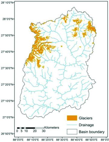
In total, 255 glaciers were mapped in the Teesta basin with a total area of 551.08 km². The glacier map of the basin is given in figure 4. The mapping of glacier is crucial in finding the vulnerability of the lakes, their position with respect to glacier. Slope of the glaciers which are attached to lakes is also an important factor, so glacier mapping has been very useful in assessing potentially dangerous lakes. In total, 143 glacial lakes have been mapped in the basin (figure 5).

Figure 5. Glacial lakes in the Teesta river basin.

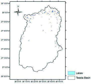
Figure 6. Lakes map overlaid on glacier map.

4.2. Potentially dangerous lakes

After applying the 0.1 km² area threshold, 37 were left to be further analysed. Lakes have been superimposed on glacier map to check for their spatial relation with respect to the glacier. As discussed in the methodology, lakes which are at the snout or are still attached to the mother glacier have been identified as shown in the figure 6.Two pairs of lakes, i.e. Lakes 63 and 65 and Lakes 58 and 59, have been found to have cascaded by each other (lying in the downstream of the other lake) as shown in figure 7. Lake 19 has two side-by-side supraglacial lakes (figure 8). After making this analysis along with others as mentioned in the methodology, in total, 18 lakes have been found to have potential to cause GLOF; all these lakes have been recorded (table 2) with their location, area, distance from the outlet of the basin, classification and reason for their vulnerability.

Table 2. Eighteen most vulnerable lakes.

Serial number	Lakes	Class	Lat–long	Area (km^2)	Distance from the outlet (km)
1	140	Moraine dammed	27° 54′ 53.26″	1.167	160.553
			88° 12′ 04.89″
2	28	Moraine dammed	27° 55′ 15.53″	0.689	165.496
			88° 09′ 51.53″
3	27	Moraine dammed	27° 53′ 44.32″	0.130	164.23
			88° 11′ 33.33″
4	38	Moraine dammed	27° 56′ 54.73″	0.279	151.814
			88° 18′ 30.40″
5	41	Valley	27° 56′ 46.32″	0.517	149.502
			88° 20′ 02.47″
6	51	Moraine dammed	28° 00′ 26.98″	0.380	155.366
			88° 29′ 50.13″
7	21	Moraine dammed	27° 51′ 14.76″	0.218	159.854
			88° 14′ 40.23″
8	19	Moraine dammed	27° 49′ 34.76″	0.372	161.673
			88° 15′ 22.96″
9	17	Blocked	27° 49′ 08.11″	0.100	161
			88° 15′ 22.96″
10	8	Moraine dammed	27° 32′ 01.48″	0.264	88.054
			88° 05′ 15.33″
11	58	Moraine dammed	28° 00′ 59.42″	0.201	150.304
			88° 33′ 56.00″
12	59	Valley	28° 00′ 32.65″	0.198	149.905
			88° 34′ 33.65″
13	69	Moraine dammed	27° 58′ 26.32″	0.559	145.051
			88° 37′ 07.00″
14	70	Moraine dammed	27° 57′ 36.55″	0.163	147.719
			88° 39′ 05.07″
15	65	Moraine dammed	28° 01′ 35.08″	1.044	166.982
			88° 42′ 58.63″
16	63	Blocked	28° 00′ 34.95″	0.805	169.569
			88° 42′ 16.28″
17	61	Moraine dammed	27° 59′ 34.95″	0.157	178.056
			88° 49′ 18.78″
18	107	Moraine dammed	27° 51′ 56.13″	0.150	132.789
			88° 52′ 12.84″

Figure 7. Cascaded Lakes 58 and 59 (Google Earth, Digital Globe).

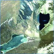
Figure 8. Presence of supraglacial lakes near a moraine dammed lake.

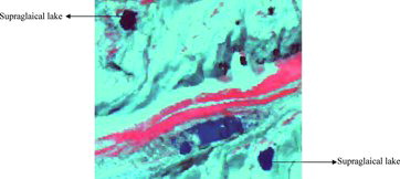
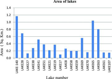
Figure 9. Area of the lakes.

4.3. Analysis for the most vulnerable lake in the basin

As discussed in the methodology, area, distance from the outlet, growth of the lake and slope have been taken into account.

4.3.1. Area

The graph (figure 9) shows areas of the 18 most vulnerable lakes identified. Although areas of all the lakes are above 0.1 km², there is a significant variation in the area of the lakes. It can be observed that 0.6 km² is the threshold dividing lakes into lakes of significant area and lakes having comparatively less area; hence Lakes 140, 28, 65 and 63 are considered as output of this stage with Lake 140 as the most important one.

Figure 10. Distance from the outlet of basin.

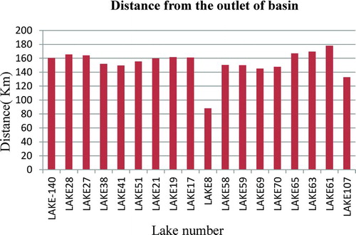
4.3.2. Distance from the outlet of the basin

As shown in the figure 10, it can be observed that distance does not play an important role here because the variation in the distance is not much prominent except for Lakes 8 and 107. Their area is less in comparison to other lakes, i.e. 0.264 and 0.150 km², so no significance can be given.

Figure 11. Graph showing percentage change in area since 2009.

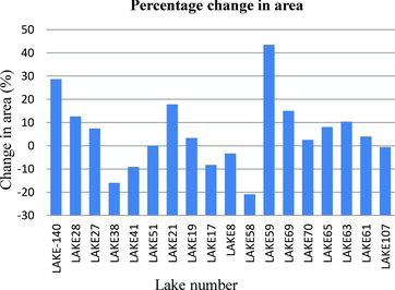
4.3.3. Growth of the lakes since year 2009

All the 18 lakes have been mapped (manually) using July 2009 Landsat image. After mapping the lakes, change detection was carried out using 2009 and 2011 mapped lake extents. As seen in figure 11, change in area is most prominent for Lake 59 followed by Lake 140, but area and hence the volume of the Lake 140 is overwhelmingly larger than Lake 59. Lake 140 expanded at an alarming rate of 28.66% since 2009.

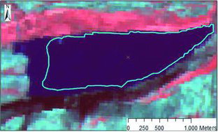
Figure 12. Lake 140 associated with the Lhonak glacier.

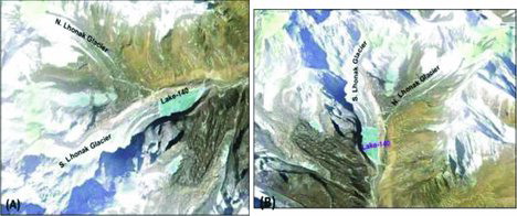
Considering all the three factors mentioned above, Lake 140 is found to be the most vulnerable lake among all the 18 lakes. This lake is associated with Lhonak glacier making it more prone to expansion in near future. It is at the snout of south Lhonak glacier (figure 12).

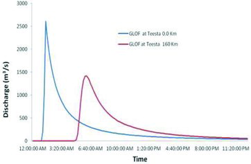
Figure 13. Flood hydrograph due to GLOF.

4.4. GLOF simulation for Lake 140

The area of Lake 140 is 1.167 km². The resulting flow due to dam breach has been routed through Teesta river. The Teesta river from glacial lake location down to the outlet (total distance is 160 km) has been presented by a number of cross-sections at an interval of 1 km, developed from the DEM. The lake volume and depth have been found to be 37 m and 42.93 Mm³ (from equations (4) and (5)). Froelich's equations yielded breach width to be 78 m and its formation time to be 3.9 hours. Owing to the rocky terrain of the Himalayas in Teesta basin, Manning's coefficient has been taken as 0.05. Breach invert level has been computed as three-fourths of the depth of the lake (which is approximately equal to the height of the dam below water surface). All the parameters generated are summarized in table 3. Figure 13 shows the flood hydrograph due to GLOF at the lake (0 km from the lake) and at the outlet of the basin (160 km from the lake). The hydrograph suggests the peak flood of 2611.136 m³/s at the lake site which gets mitigated to 1417.844 m³/s at the outlet of the basin. Flood at the lake reaches its peak 2 hours and 10 minutes after the breach of the moraine dam. The time of travel for the GLOF to reach its peak from the lake to outlet of the basin is 6 hours and 10 minutes.

Table 3. Lake 140 dam breach parameters.

Volume	Depth	Breach invert level	Breach formation time	Breach width
42.93 Mm^3	37 m	28 m	3.9 hours	76 m

Figure 14. Lake 140, change in extent from 2009 to 2011.

5. Conclusions

In the year 2011, there were, in total, 143 lakes, out of which 37 lakes were having areas greater than 0.1 km² while 106 lakes were having areas less than 0.1 km². Most of the lakes are situated above 4500 m. The area of the biggest lake, i.e. Lake 140, is increasing (figure 14) over the past years. The lake is also expanding laterally and longitudinally; therefore, this lake has been considered as a potentially dangerous lake from GLOF point of view (table 4).

Table 4. Lake 140 extent changes.

Longitudinal shift	Lateral shift	Change in area
303.66 m	66.03 m	28.66%

Simulation result shows the strength of the flood that can be caused by the outbursting of Lake 140. Table 5 shows the peak discharge at the lake and at the outlet along with the time of reach.

Table 5. Flood peak.

Location	Distance (km) from glacial lake	Total flood peak (m^3/s)	GLOF peak (m^3/s)	Travel time (hour-minutes)
At Lake 140	0	2611.136	2611.136	02-10
Outlet	160	1193.292	1417.844	06-10

GIS and remote sensing serve as a powerful tool for monitoring the glacial lakes and their health located in the remote areas. Whereas we can monitor only their area dynamics from remotely sensed images, dam break modelling provides a fair estimate of the risk in terms of peak discharge that can be caused by these GLOFs. This information can prove to be very critical for many applications such as disaster management and design of structures such as dams in downstream of these lakes.

6. Sources of error and future scope

The results and analysis done by remote sensing and mathematical modelling present an approximate solution to the real problem. There are some approximations and sources of error in modelling GLOF as follows.

1. Calculation of the volume is the main challenge in modelling GLOF using remote sensing data. There exist empirical relations between area and volume, but more accurate volume computation would come from the field investigations.

2. The inaccuracy of elevation data is another major source of error.

MIKE-11 is a 1D model and only flood hydrographs can be generated using this model. Next step would be to use a 2D model to generate flood extents resulting from GLOF. From these flood extents, much better understanding can be developed about the infrastructure that comes under the flood foot print.

References

- Bajracharya B, Shrestha AB, Rajbhandari L. 2007. Glacial Lake outburst floods in the Sagarmatha region: hazard assessment using GIS and hydrodynamic modeling. Mountain Res Dev. 27(4):336–344.
- Bloch T, Buchroithner MF, Peters J, Baessler M, Bajracharya S. 2008. Identification of glacier motion and potentially dangerous glacial lakes in the Mt. Everest region/Nepal using spaceborne imagery. Nat Hazards Earth Syst Sci. 8:1329–1340.
- Carrivick LJ. 2006. Application of 2D hydrodynamic modeling to high-magnitude outburst floods: an example from Kverkfjöll, Iceland. J Hydrol. 321:187–199.
- Froehlich DC. 1987. Embankment-dam breach parameters, hydraulic engineering. Proceedings of the 1987 ASCE National Conference on Hydraulic Engineering; 1987 Aug 3–7; Williamsburg, VA. p. 570–575.
- Hall DK, Riggs GA, Salomonson VV. 1995. Development of methods for mapping global snow cover using MODIS data. Remote Sensing Environ. 54:127–140.
- Huggel C, Kaab A, Haeberli W, Teysseire P, Paul F. 2002. Remote sensing based assessment of hazards from glacier lake outbursts: a case study in the Swiss Alps. Can Geotech J. 39:316–330.
- Jain SK, Lohani AK, Chaudhary A, Thakural LN. 2012. Glacial lakes and glacial lake outburst flood in a Himalayan basin using remote sensing and GIS. Nat Hazards. 62:887–899.
- Kulkarni AV, Bahuguna IM. 2009. Role of satellite images in snow and glacial investigations. GSI Spec Publ. 53:233–240.
- Kulkarni AV, Philip G, Thakur VC, Sood RK, Randhawa SS, Chandra R. 2001. Glacier inventory of the Satluj basin using remote sensing technique. Himalayan Geol. 20(2):45–52.
- Mool PK. 1995. Glacial lake outburst floods in Nepal. J Nepal Geol Soc. 11:273–280.
- Mool PK, Bajracharya SR, Joshi SP. 2001. Inventory of glaciers, glacial lakes and glacial lake outburst floods, Nepal. A report to ICIMOD (International Centre for Integrated Mountain Development).
- Paul F. 2000. Evaluation of different methods for glacier mapping using Landsat TM. EARSeL eProc. 1:239–245.
- Paul F, Andreassen LM. 2009. Creating a glacier inventory for the Svartisen region (Norway) from Landsat ETM+ satellite data: challenges and results. J Glaciol. 55(192):607–618.
- Paul F, Huggel C, Kääb A. 2004. Combining satellite multispectral image data and a digital elevation model for mapping of debris-covered glaciers. Remote Sensing Environ. 89:510–518.
- Quincey DJ, Lucas RM, Richardson SD, Glasser NF, Hambrey MJ, Reynolds JM. 2005. Optical remote sensing techniques in high mountain environments. Prog Phys Geog. 29(4):475–505.
- Quincey DJ, Richardson SD. 2007. Early recognition of glacial lake hazards in the Himalayas using remote sensing data sets. Global Planetary Change. 56:137–152.
- Richardson SD, Reynolds JM. 2000. An over view of glacial hazards in the Himalayas. Quaternary Int. 65/66(1):31–47.
- Saint-Venant BD. 1871. Theory of unsteady flow, with application to river floods and to propagation of tides in river channels. French Acad Sci. 73:148–154, 237–240.
- Sharma D, Singh B, Perumal M, Rai NN. 2009. Study of glacial lake outburst flood for punatsangchhu hydro electric project, Bhutan. Paper presented at: National Symposium on Climate Change and Water Resources in India; 2009 Nov 18, 19; organised by IAH, Roorkee at NIH, Roorkee.
- Teillet PM, Guindon B, Goodenough DG. 1982. On the slope-aspect correction of multispectral scanner data. Can J Remote Sensing. 8:84–106.
- Wang W, Yang X, Yao T. 2012. Evaluation of ASTER GDEM and SRTM and their suitability in hydraulic modelling of a glacial lake outburst flood in southeast Tibet. Hydrol Process. 26:213–225.
- Watanabe T, Ives JD, Hammond JE. 1994. Rapid growth of a glacial lake in Khumbu Himal, Himalaya: prospects for a catastrophic flood. Mountain Res Dev. 14(4):329–340.
- [WECS] Water and Energy Commission Secretariat. 1987. Study of glacier lake outburst floods in Nepal Himalaya. WECS Interim Report. Kathmandu: WECS.