Landslide monitoring using multitemporal terrestrial laser scanning for ground displacement analysis

Abstract

In the analysis of the temporal evolution of landslides and of related hydrogeological hazards, terrestrial laser scanning (TLS) seems to be a very suitable technique for morphological description and displacement analysis. In this note we present some procedures designed to solve specific issues related to monitoring. A particular attention has been devoted to data georeferencing, both during survey campaigns and while performing statistical data analysis. The proper interpolation algorithm for digital elevation model generation has been chosen taking into account the features of the landslide morphology and of the acquired datasets. For a detailed analysis of the different dynamics of the hillslope, we identified some areas with homogeneous behaviour applying in a geographic information system (GIS) environment a sort of rough segmentation to the grid obtained by differentiating two surfaces. This approach has allowed a clear identification of ground deformations, obtaining detailed quantitative information on surficial displacements. These procedures have been applied to a case study on a large landslide of about 10 hectares, located in Italy, which recently has severely damaged the national railway line. Landslide displacements have been monitored with TLS surveying for three years, from February 2010 to June 2012. Here we report the comparison results between the first and the last survey.

1. Introduction

Landslides are a major natural hazard in many countries (http://www.safeland-fp7.eu/Pages/SafeLand.aspx). Geomatic techniques give a great contribution to the knowledge of both the surface shape and the kinematics of landslides providing data which are used by geologists, geomorphologists and geotechnics for interpreting the phenomenon. Among all the geomatic techniques, remote sensing ones are undergoing rapid developments. The possibility of acquiring three-dimensional (3D) information of the terrain with high accuracy and high spatial resolution is opening up new ways of investigating the landslide phenomena. The two major remote sensing techniques that are exponentially developing in landslides investigation are ground-based interferometric synthetic aperture radar (GBInSAR) and light detection and ranging (LiDAR) (Carter et al. 2001; Slatton et al. 2007; Heritage & Large 2009). The joint use of terrestrial laser scanning (TLS) and GBInSAR techniques may help to understand landslide phenomena, as is discussed in Teza et al. (2008).

Since the mid-1990s, the LiDAR technique has indeed played a central role in the detailed measuring of natural environments and thus several applications in landslide investigation have been developed. The number of publications discussing the use of LiDAR in landslide studies has grown considerably during the last decade. The LiDAR technique is very interesting for its applications in landslide hazard analysis thanks to its ability to produce accurate and precise digital elevation models (DEMs) of land surface.

Especially terrestrial laser scanners (TLSs) have the advantage to provide huge amounts of data at high resolution in a very short time and then they allow a precise and detailed description of the scanned area (Pirotti et al. 2013a; Slob & Hack 2004).

The technique seems indeed to be very suitable for landslides deformation measurements, especially for terrains with difficult access and steep slopes, since multiple surveys enable rapid 3D data acquisition of the landslide surface. A detailed overview of LiDAR techniques applied to landslides is contained in Jaboyedoff et al. (2012).

Main applications to the landslides range from mapping and characterization (Derron & Jaboyedoff 2010; Guzzetti et al. 2010) to vegetation mapping (Teza et al. 2007; Abellan et al. 2009; Prokop & Panholzer 2009; Abellan et al. 2009; Barbarella & Fiani 2012, 2013; Pirotti et al. 2013b).

For DEM generation it is essential to extract the bare soil data from the whole dataset. Data editing requires a large amount of work; without this effort, however, it is not possible to use the data for a quantitative precise analysis of the movements.

This task consists of a classification of the data coming from laser scanners into terrain and off-terrain classes. Due to the huge amount of data that is generated by the laser scanning techniques, there is a need to automate the process. A detailed overview of both several filter algorithms developed for this task and a representative selection of some methods is contained in Briese (2010). TLSs belonging to the last generation of instruments allow acquiring more echoes; for example, Riegl VZ series instruments are full waveform systems. They can provide, if properly equipped with software tools, a full waveform analysis very effective for the filtering of the vegetation (Mallet & Bretar 2009; Elseberg et al. 2011; Guarnieri et al. 2012; Pirotti et al. 2013c).

Subsequently, it is necessary to convert the irregularly spaced point data into a DEM which can be generated by appropriate interpolation methods (Kraus & Pfeifer 2001; Vosselman & Sithole 2004; Pfeifer & Mandlburger 2009). The accuracy of a DEM and its ability to faithfully represent the surface depends indeed on both the terrain morphology and the sampling density and also on the interpolation algorithm (Aguilar et al. 2005).

If the goal of the survey is to monitor the ground deformation over time, two or more DEMs have to be compared in order to monitor the displacements of a number of points of the terrain (Fiani & Siani 2005; Abellan et al. 2009). Here a number of different approaches can be used. For instance one can directly compare the DEMs obtained over time by simply fixing a number of points belonging to particular objects visible in the two different point clouds (Ujike & Takagi 2004); the estimated transform parameters can then be used in order to transform all the points of a cloud in the reference system of the other one, making possible a comparison between them (Hesse & Stramm 2004).

A more general approach allowing a full 3D analysis useful for point clouds comparison is based on the algorithm called LS3D, proposed by Gruen and Akca (2005). The authors themselves have introduced a number of variants so as to make it more efficient. The algorithm is based on the principle of least squares adjustment; it makes use of statistical criteria for both outlier detection and the evaluation of the adjustment quality.

Among the available surveying techniques, TLS has the least standardized operating protocols, probably due to being a surveying technique younger than others. In order to overcome this gap, in this paper, we describe the approach we used for TLS surveying and data processing on a “real world” study case, i.e. a large landslide that presents many criticalities in the monitoring over time. The presence of thick vegetation, the difficulties in TLS positioning for a good visibility, the instability of the hillslope from which we are able to make the surveying measurements, the availability of practically no “stable” areas around the landslide are all causes that make both the survey campaigns and data elaboration very hard.

In this paper we describe the methodological approach we used in order to overcome some criticalities of the surveying technique. As for the need of a reference system stable over time, we connected the targets to a number of permanent stations belonging to the network established for real-time survey. These stations are monitored continuously and are now widely used in many countries. A GPS survey now is easy to perform and it is not expensive. Since permanent stations are far away from the landsliding area, the baseline error is not so small; nevertheless, it is doubtlessly acceptable if you think the increase of accuracy due to the stability of a reference system that is monitored over time on wide areas.

With regard to the reconstruction of a grid starting from the point clouds, given the importance to identify the best algorithm, we made a number of tests on a check sample extracted from the whole point clouds. We present the result of the comparison of various surface-fitting algorithms in order to evaluate the quality of the interpolation in our operational context (taking into account both the terrain morphology and the huge density of points).

Finally, in order to compare terrain surfaces acquired at different epochs in terms of mobilized volumes, it is our opinion that a “differential” approach to homogeneous areas would provide more information than usual surface comparison techniques.

As a matter of fact, a segmentation of the grid resulting from surface difference in several areas characterized by the same behaviour would allow a quantitative analysis of displacements occurred over time and this information could be useful to geomorphologists to better interpret the phenomenon.

2. The Pisciotta landslide

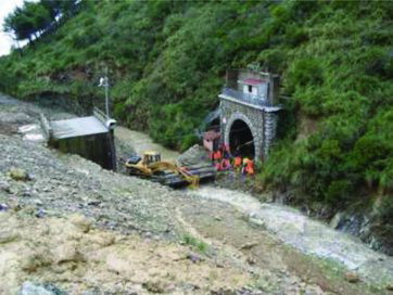
The phenomenon we are considering is taking place in Pisciotta (Campania Region, Italy), on the left side of the final portion of the Fiumicello stream, and causes extensive damage to both an important state road and to two sections of the railway line connecting North and South Italy (close to Cilento). The consequences of these movements are visible on a long stretch of road that appears to be completely disrupted (figure 1). Not long ago, due to a reactivation landslide event, the railway has been endangered and disrupted by landslide dam break just upstream: mud and soil brought by the landslide dam break into the river after heavy and prolonged rains have caused the blockage of both tunnels and the interruption of rail traffic on the main north-south railway line in Italy for about one day (figure 2).

Figure 1. State Road 447 deformations and ruptures.

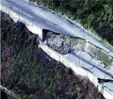
Figure 2. Dam break by Pisciotta landslide local reactivation that caused the interruption of the rail traffic in the odd track of the Salerno-Reggio Calabria railway and the obstruction of the stream. The catastrophic event occurred during the period December 2008–January 2009. In the picture, you can see the railway tunnel and the rescue personnel at work (belonging to both the Italian State Railways and Civil Protection Department).

According to the widely accepted and used definition for landslide as ‘‘the movement of a mass of rock, debris or earth down a slope’’, established by Cruden (1991) and Cruden and Varnes (1996), the active Pisciotta landslide is defined as a landslide system with a deep seated main body affected by long-term, rototranslation, slow displacements and on it secondary earth slide-flow with an intermediate sliding rupture surface and shallow, rapid earth flows (Coico 2010; Guida & Siervo 2010; Coico et al. 2011).

Our case study is a wide area of nearly 10 hectares. Since 2005, when the ground movement monitoring started, a traditional topographical survey has been performed by materializing a set of vertexes on the landslide body and controlling its position: this was done by measuring angles and distances from the slope facing the area. These operations allowed a first estimate of the magnitude of the ground movement, but such a control network is not sufficient to describe mass movements and changes in the shape of the slope. The first surveying campaigns were carried out by “Provincia di Salerno” (PdS), that is the management authority for the road damaged by the landslide; a specialized company, Iside Srl, is monitoring the landslide trend on behalf of PdS. The phenomenon monitoring activity was carried out from 2005 to 2009 using topographic and geotechnical methods (Iside 2007); it was mainly oriented to the monitoring of the area close to the road. The monitoring system they realized was basically made up of a number of sensors, like fixed weather stations, piezometers, inclinometers, strain gauges and of a topographical network.

In the period 2005–2009, two topographical surveys per month were performed.

The results of the periodic surveys show that the amount of planimetric displacements in a period of about four years is about 7 m while the altimetric one is 2.5 ÷ 3.5 m. The average daily speed of the landslide is approximately 0.5 cm per day with peaks of up to 2 cm per day in planimetry and of about 0.2 cm per day with peaks up to 1.5 cm per day in height. The movements were measured with respect to two pillars (here called I1, I2) placed on the opposite hillside of the valley; the upper part of the sliding slope is visible from them.

In such a way it is possible to determine reliably and accurately the movements of the single observed points and to obtain information on the dynamics of the phenomenon, but is quite impossible to compute the correct amount of the moving material or to define precisely the area affected by the landslide.

2.1. TLS surveying campaigns

The goal of the survey campaigns we had been running from 2010 to 2012 was to describe numerically the terrain morphology of the landsliding slope and its variation over time. For this purpose we decided to use the TLS surveying methodology in order to obtain a reliable 3D model of the landslide surface (Barbarella & Fiani 2012; 2013).

Monitoring requires a strict programme of surveying and data processing methodologies that can be repeated systematically at different times, always avoiding changing any detail of the procedure. If this is not done the differences in the details of the procedures can falsify the real movements and deformations of the object.

We carried out a TLS “zero” survey and about four months later a repetition measurement using a long-range instrument, Optech ILRIS 36D; a further surveying campaign was carried out one year later by using two different instruments, a long range (Riegl VZ400) and a medium range one (Leica Scanstation C10). The last campaign dates back to June 2012. Here we used both Optech and Leica instruments.

The rugged morphology of the surveyed area has been a strongly conditioning element in the choice of the sites where the stations have been placed. The strong dynamics of the landslide implies that the measurement campaigns have to be carried out in a very short period of time. This is why we ran both the TLS and the GPS surveys during the same day. Each surveying campaign lasted 2–3 days.

In all our survey campaigns we have recorded laser scan measurements acquired from several TLS stations, located on the stable slope at different altitudes, in order to measure both the upper and the lower parts of the landslide, downstream; here distances are smaller and short-range instruments can be used, obtaining a larger density of points. At the toe of the landslide there is a railway bridge connecting the two tunnels and the terrain above the entrance of the tunnel can be measured with high accuracy; not far from this, towards the valley, there is a longer bridge and a tunnel.

In each scan, we use a number of targets in order to frame the whole survey in a given reference system. The coordinates of both the target and the TLS stations were measured by GPS receivers in static mode keeping fixed the coordinates of two vertices.

In better details, as for the survey frame

• the targets and the TLS stations have been surveyed by GPS baselines referred to a “near reference” system;

• the “near reference” system consists of two pillars materialized on a concrete wall in the stable area located at walking distance from the survey one;

• the two pillars were themselves connected to two permanent stations belonging to a network real-time kinematic (NRTK) for real-time surveying service of the Campania Region, far away 26 (Castellabate) and 38 (Sapri) km from the landslide.

In view of the distance between the landslide areas we made continuous GPS observations during two days.

We used different types of targets, both spherical and of the type suggested by the software vendors (cylindrical and plane) for easy recognition when using the processing software. The “final” coordinates of the targets came from a least-squares adjustment in ITRF05.

In this paper we considered only the data acquired with the same instrument Optech from the two measurement campaigns more temporally distant, i.e. in February 2010 and in June 2012.

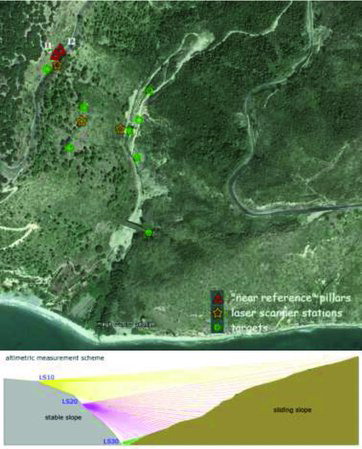
In figure 3 (upper panel), one can see the positions of the “near reference” pillars (red triangles), of the TLS station points (orange stars) and of the targets (green circles). In the panel below, we show the altimetric scheme of the same campaign with the different areas analysed with the different tilts. For the first campaign the measurement scheme is almost similar.

Figure 3. 2012 survey. In the upper panel we show the location of the “near reference” pillars (elaboration from Google Maps^TM), the laser scanner stations and the targets. In the panel below we show the altimetric scheme of the same campaign.

2.2. Data processing

The initial phase of the data processing from surveys aims at determining the positions of both targets and TLS stations in the selected reference framework. In this way all the scans will be referred in a specific frame and we will be able to compare them over time. The first step of the process is the connection between the reference stations of the NRTK network taken as fixed points and the two pillars of the near reference frame.

The second step concerns the connection between both targets and laser stations and the pillars assumed as fixed. We also perform a data snooping analysis on the results of the minimum constraint adjustment of the GPS network; this analysis detected two blunders in the 2012 measurement set. The final target coordinates were determined in ITRS05. Table 1 shows the values (in cm) obtained for the standard deviations of the adjusted geographic coordinates of the two pillars I1 and I2, and a summary of the values obtained for the standard deviations on the targets. The level of accuracy we have achieved for the survey of 2012 is lower than the one achieved for the previous surveys.

Table 1. Standard errors on pillars and targets.

	February 2010			June 2012
Standard deviation (cm)	σφ	σλ	σh	σφ	σλ	σh
Pillars
I1	0.4	0.4	0.9	0.5	0.4	1.4
I2	0.3	0.3	0.8	0.6	0.5	1.5
Targets
Mean	0.3	0.2	0.6	1.3	1.0	4.0
Standard deviation	0.1	0.1	0.3	0.2	0.3	1.3
Max value	0.1	0.1	0.2	1.4	1.4	5.6

For the data coming from TLS the processing steps are: scans alignment, editing and georeferencing. We used PolyWorks software package for data processing.

The alignment step is very important for the metric quality of the final product.

One must take special care in the scan pre-alignment phase, especially in the choice of the area overlapping between adjacent clouds and of homologous points. This phase, called co-registration, is mathematically realized by a six-parameter transformation before the best-fitting alignment final step, usually based on the “iterative closest point” algorithm. The Optech ILRIS 36D TLS instrument records multiple tasks for each cloud (each one with a width of 40 × 40 deg). When the instrument is well calibrated and rectified all tasks should be in a single reference system. Nevertheless, we have decided to set a large overlap between tasks in order to check the effectiveness of this automatic co-registration.

From an operational point of view, first we aligned all the tasks referred to each scan collected with a specific tilt from every TLS station.

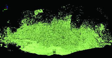
Alignment procedure has been performed by locking the central task and then adding one by one, one to the right and one to the left of the central one, the further tasks, so as to minimize the effects of error propagation. Once having reassembled all the scans acquired with different tilts from the same TLS station, we have added also the more detailed scans acquired over the targets. At last, all the scans have been aligned, producing a single global scan describing that specific measurement campaign. In figure 4, we show the aligned clouds of the last survey (July 2012).

Figure 4. Whole point clouds obtained during the 2012 survey campaign.

The resulting scans must be edited in order to remove from the dataset all the points not belonging to the bare soil; in our application, this concerns essentially the vegetation, but also artefacts. For example, the points inside the tunnel have to be removed from the dataset. The next step of data processing is the scan georeferencing in a single reference system. Especially when there are no terrain details that can be considered stable and that are placed in a suitable position within the cloud, a precise georeferencing of the cloud in each epoch is of course a critical step.

We made a six-parameter transformation in order to georeferencing all the scans; a seven-parameter transformation (conformal transformation) gives almost the same results. We note that usually the laser data processing software packages do not provide a rigorous analysis of the quality of the standardized residuals of the transformation. The process of georeferencing has led to values of 3D residuals ranging from 5 to 6 cm.

Once these steps have been done, two point clouds that describe the landslide surface in two different epochs are available. Since all the surveys have been framed in the same reference system, it will be possible to compare the digital terrain models (DTMs) elaborated starting from the point clouds obtained at different times.

3. Method validation and control procedures

Deformation analysis requires that the data collected during repeated surveys were framed in a common reference system that must be stable over time. If a number of stable details are in the neighbourhood or inside the surveyed area, they can be used for georeferencing all the scans and thus make the surveys comparables. If no detail within the point cloud may be considered undoubtedly stable, the need to refer the surveys to far stable areas arises.

Once all the point clouds are framed in a common reference system, we can compare them over time. To do this we need a DEM that represents the earth's surface. The DEMs can be in the form of triangulated irregular network (TIN) or grid. While TINs are generally built applying the Delaunay criterion, in order to create a grid we have to choose an interpolation algorithm to calculate the grid node values starting from the sparse point clouds. The accuracy of a DEM and its ability to faithfully represent the surface depends on the terrain morphology, the sampling density and on the interpolation algorithm (Fiani & Troisi 1999; Aguilar et al. 2005; Kraus et al. 2005; Pfeifer & Mandlburger 2009).

This raises the question of how the different interpolation methods used in order to reconstruct the terrain surface are able to produce very different shapes. With this goal in mind we performed a number of tests comparing the surfaces built using several DEM interpolation methods on the same sample of data.

3.1. Absolute referencing and its reliability

In our case study, the only detail in the whole scene that can give us some assurance of stability over time is the entrance of the tunnel located on the landslide toe. It is nevertheless not large enough and peripheral in the scan to guarantee a correct georeferencing of the whole area.

Since even the two pillars that have been built outside the landslide give us an a priori stability guarantee, they have been connected to two vertices belonging to the network of GPS permanent station for real-time survey. These permanent stations (PSs) are therefore monitored continuously.

The connection with reference points located far away from the area causes a large uncertainty in the position of the targets; the situation is however improved by the fact that the reference frame is stable. The result of the GPS baselines adjustment gives the values shown in table 1 for the standard deviations of the target coordinates for a single survey. The error on the differences of the coordinates measured in the two surveys taken at different epochs, if no systematic or gross error occurred in the dataset, amounts at one and half times the above value.

Both the bridge and the mouth of the tunnel do not show any evidence of deformation occurred. So they can be used as stable details to check on them the absolute georeferencing of the data coming from the two periods, allowing us to estimate the local shift. This is probably due to the error in the estimation of the baselines between the pillars and the fixed points that are far away. We have been able to evaluate the amount of the difference of the position of the same detail by comparing the coordinates of a number of “homologous” points identified on the artefact. The coordinate differences between the very few points, really “homologues” belonging to the two scans (2012 and 2010), reached 6, 4 and 4 cm on average, respectively, in the north, east and height components, with standard deviations of the means of 2 cm on average for all three.

The comparison between the heights of the points located on the top of the tunnel confirmed the magnitude of the coordinate differences (see Section 4). We therefore could evaluate the overall georeferencing error (locally) within 10 cm. It is not possible to cancel this error but we can reduce its effect performing a rigid body transformation, i.e. a translation of the amount previously found. We made this before the comparison between scans. Then we made the comparison in order to obtain the differences over time between both surfaces and volumes or the profiles, we should therefore take in account an uncertainty in the coordinates of the order of nearly 5 cm, due to the georeferencing step.

3.2. Surface reconstruction via interpolation

There are many interpolation algorithms for generating surface grid-based DEM. In landslide analysis the choice of the algorithm is not obvious, depending on various factors as terrain morphology and presence of discontinuities. The assessment of the surface deformation occurred over time is strongly influenced by the DEM construction mode.

For the choice of the interpolator we used a very simple criterion, i.e. the degree of adherence of the interpolated surface to the original data used to generate the surface.

For this we calculated the deviation of the laser points from the interpolated surface.

The difference between the height z of the point and the interpolated height z_int(x_k,y_k) is here called residual. We made our tests on sample data related to the landslide toe. We chose this area since it is both without vegetation and quite complex; an artefact, i.e. the mouth of a tunnel is visible in the scene (figure 5).

Figure 5. The data sample we tested, extracted from the full mesh obtained by the alignment of the point clouds (2012 survey campaign).

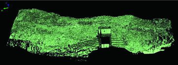
The sample consists of about 4 million points; we extracted from it one point every one hundred one (by decimation). We then calculated the height differences between the N points belonging to this check sample and the interpolated surface built starting from the remaining 99% of the data.

We tested the following algorithms widely used in the modelling of surfaces and frequently present in several software packages (the acronym we used is written in parentheses):

• Inverse distance to a power, second degree (Idw2)

• Kriging, linear variogram (Kri)

• Natural Neighbor (NatNe)

• Local polynomial, first and second degree (LP1°, LP2°)

• Radial basis function, multiquadric, smoothing factor 0 (RBF0), 0.0001 (RBF0001), 0.0013 (RBF0013) and 0.01 (RBF01).

A few checkpoints give residuals with very high absolute values. These points are mainly located in areas characterized by rapid changes in morphology (the tunnel wall, abrupt slopes, etc.). However, the residuals exceeding 1 m have been considered outliers; their percentage ranges from 3.8% to 5.5%. Some researchers have tended to use the root mean square error (RMSE) as a global measure of a DEM's accuracy (Yang & Hodler 2000). Since a few outliers are present in our sample, we have considered the number of events that fall in certain ranges of values, precisely the checkpoints that have height value with respect to the fitted surface ranging from 5 cm to 1 m unlike the RMSE in order to evaluate the performance of the various interpolators. This operation has been done for all the algorithms aforesaid.

In table 2 we show the relative frequency of the residuals (in percentage on the total of n points, including outliers) for the ranges we took in account. Here we report only the residual values that range from 5 to 25 cm, in steps of 5; in the last column you can see the percentage of values that fall under one meter.

Table 2. Relative frequency of the absolute values of the residuals, divided into ranges. The percent value is computed on the whole sample of check points.

	% of check points
Algorithm	5 cm	10 cm	15 cm	20 cm	25 cm	1 m
Idw2	73.5	84.6	88.6	90.5	91.7	96.2
LP2°	73.8	84.6	88.4	90.3	91.4	95.7
RBF0	73.2	84.3	88.4	90.3	91.5	96.1
LP1°	73.5	84.4	88.3	90.2	91.5	95.9
NatNe	73.3	84.2	88.3	90.3	91.4	96.0
Kri	73.0	84.0	88.2	90.2	91.4	96.1
RBF0001	67.1	80.0	85.0	87.5	89.1	94.8
RBF0013	65.9	79.1	84.3	87.1	88.6	94.5
RBF01	67.1	76.2	81.7	84.6	86.5	94.4

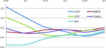
If we compare the algorithms in terms of their performances in domain adaptation, the best are Idw2, local polynomial and radial basis function (with smoothing factor sf = 0), even if the differences between them are substantially quite small. More in detail, the height differences between the checkpoints and their interpolated value are greater than 20 cm in less than 10% of the sample; almost 85% of the residuals are less than 5 cm in absolute value. The graph of figure 6 shows the behaviour of the algorithms. The percentage differences between each algorithm we tested and the Idw2 are given. The intervals we considered range from 5 to 30 cm.

Figure 6. Percentage differences between the different interpolation algorithms we tested and inverse distance to a power (Idw2).

In view that a few algorithms give results quite similar, the ability to insert the breaklines has also been taken into account in the choice of the algorithm to use. Breaklines (or similarly defined characteristic lines, skeleton lines or faults) are, as well known, linear elements that describe changes in smoothness or continuity of a surface.

Breaklines are usually used in order to describe extreme local occurrences and thus complete the overall terrain structure and its digital representation. Their preservation and integration in the database is essential to obtain a reliable DEM (Lichtenstein & Doytsher 2004).

In our case study this ability may be useful to describe the edges of the facing of the tunnel. For this reason too we chose the algorithm inverse distance to a power in order to get the interpolated surface of the landslide.

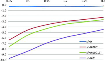
It is also noteworthy that radial basis function algorithm with multiquadric basis function has not produced the best fit (on the basis of the criterion we adopted). As Mongillo (2011) noted, the choice of the value of smoothing factor is critical; in our tests first we chose a value equal to 0.0001, then a value purposely too high, i.e. 0.01, and finally the value of 0.00013, which has been suggested by a software based on the criterion where d is the length of diagonal of the data extents and n is the number of points.

In figure 7, the graph of the differences between radial basis function and inverse distance to a power varying the smoothing factor parameter is shown.

Figure 7. Percentage differences between the algorithms radial basis function and inverse distance to a power varying the smoothing factor (sf) parameter.

To conclude, the following analysis is referred to a grid DEM built by means of Idw2 algorithm; we designed the breaklines only in correspondence of the mouth of the tunnel, which is the sole artifact present in the scans.

4. Results

4.1. Surface comparison

A first comparison between the two point clouds could be performed considering as a reference surface the interpolated mesh of one of the two clouds. A triangular mesh is the polygonal surface obtained triangulating the points of a cloud (triangular irregular network).

In order to follow the evolution of the landslide morphology here, it has been chosen to consider the 2010 surface as the reference one. The “Compare” procedure implemented in PolyWorks consists in measuring the distance of each point of a cloud with respect to a reference surface.

Distances could be measured in several ways, with respect to different directions, considering a certain angle and search radius defined by the user. Here it has been chosen to measure distances along the shortest path from the point to the surface.

The sign of the distance depends on the relative position of cloud and mesh: if a point is above the mesh the distance is positive (in this case it corresponds to accumulation of debris, represented from yellow to brown in figure 8); otherwise, if it is below the mesh, the sign is negative (“erosion”, from light to dark green; the meaning of the term “erosion” will be better explained in the following).

Figure 8. Comparison of 2012 point clouds with respect to the 2010 reference mesh.

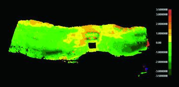
At the end of this process input data points are represented in a chromatic scale whose entities correspond to the distance values. The result shown in figure 8 was obtained considering a search radius of 3.5 m, the process has been performed in terrain coordinates. The results of a comparison procedure like this are suitable for a quick identification of stable/unstable areas but do not allow performing metric estimates of mobilized volumes.

4.2. Cross sections

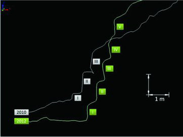
A quantitative analysis of the variations in terrain surfaces is possible comparing cross sections of interpolated meshes; following the indications of the geomorphologists who are studying the landslide, several cross sections have been taken, one of which is shown in figure 9.

Figure 9. Profile of the hillslope affected by landsliding from the midslope to the toeslope. The section has been drawn near the railway tunnel.

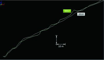
Allowing a high degree of detail in representation along parallel profiles of a landslide, cross sections represent one of the most useful tools for geomorphologists. Several cross sections have been taken, measuring the differences along the vertical between the two profiles.

From February 2010 to July 2012 the variation in height (thickness) measured in some points of the processed sample has nearly reached 3.5 m.

4.3. Mobilized volumes

In the study of a landslide, the knowledge of the amount of debris mobilized in a certain period is very important. In commercial software packages oriented to TLS data processing, this result is often achieved differencing the volumes comprised between the interpolated surfaces and a horizontal reference plane. Anyway information related to the global volume could be not representative of relative displacements between portions of the landslide.

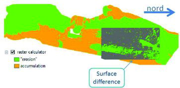
For this reason it is advisable to perform volume calculations considering homogenous areas with respect to the relative position (below/above) of the two surfaces (figure 10). This classification has been performed in a GIS environment using a raster calculator (analogous results have been obtained in ArcGIS considering TINs, using a Surface Difference tool).

Figure 10. Automatic segmentation into two classes: in green, points in accumulation, in orange points corresponding to excavation; being interested by vegetation, the depletion zone of accumulation points is not comprised in the processed sample. The class of “stable” points here has been omitted for sake of clarity. Similar results have been obtained in the sample area on the right subtracting the two TINs, as pointed out by the continuity in colours.

The two scans have been first interpolated with an inverse weighted distance algorithm with a second-order exponent applied to the distance (Idw2), and 20 cm cell width. The search radius has been of 2 m, considering a neighbourhood of 64 points. The cell width has been chosen accordingly to the mean span of the points in both the surveys. The main geometries of the railway tunnel have been considered as hard breaklines in the interpolation.

The grids corresponding to interpolated surfaces have then been differenced, subtracting the 2010 one to the 2012 one (figure 11). To distinguish areas in erosion from those of accumulation, the resulting grid has been classified into three classes:

Figure 11. Grid obtained subtracting the 2010 surface to the 2012 one, in dark green the 3D breaklines corresponding to the main geometries of the railway tunnel. Palette: cells with colours from blue to green correspond to “erosion” areas, cells from yellow to brown cells to accumulation ones.

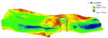
• −0.1 ÷ 0.1 m, representing the points which could be considered stable;

• ≥ 0.1 m, points in accumulation from 2010 to 2012 (e.g. 2012 surface is above the 2010 one);

• ≤ −0.1 m, points in “erosion” (e.g. 2012 surface is below the 2010 one).

The threshold of 10 cm for stable/unstable points corresponds to a rough estimate of the overall precision of the method (deriving from alignment, georeferencing, interpolation and comparison accuracy).

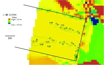
It has to be noted that the difference values in points corresponding to railway tracks are around zero: given the intrinsic stability of the tracks this fact could be considered as an evidence of georeferencing quality and correction shift appropriateness (figure 12).

Figure 12. Contours extracted from the 2012–2010 difference grid, considering the tunnel main geometries as breaklines (in black), with a sampling interval of 5 cm; the contours corresponding to railway tracks are comprised from 0 to 10 cm. The yellow colour in the grid corresponds to difference values around zero.

The term “erosion” here should not only be interpreted as landslide displacement or as weathering, but also as an effect of removal of landslide debris which could dam the Fiumicello creek and the nearby gravel road.

Then the corresponding volumes have been calculated, resulting in 297 m³ of total accumulation and 2148 of total “erosion”, mainly due to excavation. The total volume corresponding to points considered as stable (from −0.1 m to 0.1 m of difference) is about 3.5 m³, i.e. a negligible amount.

The area around the tunnel has not been considered in volume calculations, in order not to affect the results with spurious differences deriving from the different acquisition geometries of the two scans. As previously mentioned, railway tunnel and tracks could be considered the only stable part of all the scenery. As expected, “stable” points are located near the railway tunnel and between accumulation and erosion areas.

These results are in agreement with the comparison performed in PolyWorks, taking into account the different directions considered in calculations (along the vertical in DTM comparison, along the shortest path from the point to the reference mesh in PolyWorks). This classification represents a sort of rough segmentation, which would had been the proper way to study the landslide in all its aspects but it would have required specific algorithms.

In 2011, in the framework of the actions taken to stabilize the toe of the landslide, the concrete blocks of the retaining wall on the right of the tunnel were removed and repositioned, passing from three to five rows. This change is not clearly noticeable in the comparison results, probably because the surface of the reference mesh is continuous and more or less the blocks are positioned along the steepness of the slope.

Only a few anomalies have been pointed out by some patches clearly different from the surrounding areas, with irregular shapes not corresponding with the geometry of an ashlar (figure 13). Conversely, this intervention is evident in cross sections, as shown in figure 14.

Figure 13. Comparison results over the ashlars nearby the railway tunnel.

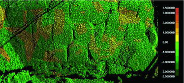
Figure 14. Cross section taken along the concrete blocks of the retaining wall, close to the railway tunnel.

5. Discussion and conclusions

The survey of a landslide slope often requires more than one scan to overcome visibility issues but with respect to other techniques, allows the acquisition of a huge amount of data in a relatively small time.

In case the objective is to monitor the slope over time, a crucial aspect is to identify a reference system which is stable over time. If no stable elements with such characteristics are to be found in the point cloud, it is necessary to identify and use points located outside the point cloud, even if located at a distance, if they are stable over time.

Given the lack of stable reference benchmarks nearby the landslide, georeferencing could be made with respect to continuously operating reference stations, today present in many countries, which are continuously monitored over wide areas for their intrinsic consistency.

Connection to targets by global navigation satellite systems (GNSS) receivers implies some uncertainness in the determination of point positions, in this case about 5 cm in each coordinate; this estimate has been assessed considering the difference in positions of homologous points in the two surveys identified in the only stable object present in the scenery, the railway tunnel.

The processing of the acquired clouds is undoubtedly the most time consuming task of the entire work, not only for the co-registration of the several scans constituting each single cloud, but also for surface reconstruction from clouds.

In case of DEM production over a grid, it is worthwhile an evaluation of which algorithm allows the better interpolation of the scanned surface, depending on landslide morphology and on points density.

Several tests performed over a check sample of points not considered in the interpolation have indicated the inverse square distance weighted as the most suitable algorithm. These tests have also confirmed the sensitivity of radial basis function algorithms to the proper smoothing factor.

Displacements detection could be performed considering DEMs, both in TIN or in grid format: in order to obtain useful results for understanding the phenomenon, there is the need to perform not only surface comparisons (for instance rendering a cloud with a chromatic scale of point to mesh distances) but also to take cross sections, which could point out variations in shape otherwise not clearly noticeable.

In this case, cross sections allow to detect (with quantitative estimations) human interventions in the blocks of the retaining wall that otherwise would be not so easily understandable in point to mesh comparisons.

Evaluation of mobilized volumes is all the more interesting for the morphological analysis as much as possible on areas run by a homogeneous behaviour.

An attempt for an automation (even if only partial) of segmentation of the difference grid still remains an open problem.

References

- Abellan A, Jaboyedoff M, Oppikofer T, Vilaplana JM. 2009. Detection of millimetric deformation using a terrestrial laser scanner: experiment and application to a rock fall event. Nat Hazards Earth Syst Sci. 9:365–372.
- Abellan A, Vilaplana JM, Calvet J, Blanchard J. 2010. Detection and spatial prediction of rock falls by means of terrestrial laser scanning modelling. Geomorphology. 119:162–171.
- Aguilar FJ, Agüera F, Aguilar MA, Carvaj F. 2005. Effects of terrain morphology, sampling density, and interpolation methods on grid DEM accuracy. Photogrammetric Eng Remote Sensing. 71:805–816.
- Barbarella M, Fiani M. 2012. Landslide monitoring using terrestrial laser scanner: georeferencing and canopy filtering issues in a case study. Int Arch Photogramm Remote Sens Spatial Inf Sci. XXXIX-B5:157–162. Available from: www.int-arch-photogramm-remote-sens-spatial-inf-sci.net/XXXIX-B5/157/2012/isprsarchives-XXXIX-B5-157-2012.pdf
- Barbarella M, Fiani M. 2013. Monitoring of large landslides by terrestrial laser scanning techniques: field data collection and processing. Eur J Remote Sensing. 46:126–151.
- Briese C. 2010. Extraction of digital terrain models. In: Vosselman G, Maas HG, editors. Airborne and terrestrial laser scanning. Dunbeath: Whittles; p. 135–167.
- Carter W, Shrestha R, Tuell D, Bloomquist D, Sartori M. 2001. Airborne laser swath mapping shines new light on earth's topography. EOS Trans Am Geophys Union. 82:549–555.
- Coico P. 2010. Hydrogeological disaster multirisk hotspots: methods and identification [dissertation]. Naples (IT): University of Naples Federico II.
- Coico P, Calcaterra D, De Pippo T, Di Martire D, Guida D. 2011. A preliminary perspective on landslide dams of Campania region, Italy [abstract]. The Second World Landslide Forum. Oct 3–9; Rome (IT).
- Cruden DM. 1991. A very simple definition for a landslide. IAEG Bull. 43:27–29.
- Cruden DM, Varnes DJ. 1996. Landslide types and processes. In: Turner AK, Schuster RL editors. Landslides: investigation and mitigation, Transportation Research Board Special Report 247, National Research Council. Washington (DC): National Academy Press; p. 36–75.
- Derron MH, Jaboyedoff M. 2010. LIDAR and DEM techniques for landslides monitoring and characterization [preface]. Nat Hazards Earth Syst Sci. 10:1877–1879.
- Elseberg J, Borrmann D, Nuchter A. 2011. Full wave analysis in 3D laser scans for vegetation detection in urban environments. Proceedings of the XXIII International Symposium on Information, Communication Automation Technologies; IEEE Xplore, ISBN 978-1-4577-0746-9. 2011 Oct 27–29; Sarajevo (Bosnia and Herzegovina).
- Fiani M, Siani N. 2005. Comparison of terrestrial laser scanners in production of DEMs for Cetara tower. CIPA 2005 XX International Symposium; 2005 Sep 26-Oct 1; Torino (Italy). Available from: http://cipa.icomos.org/fileadmin/template/doc/TURIN/277.pdf
- Fiani M, Troisi S. 1999. DEM's comparison for the evaluation of landslide volume. Proceedings of ISPRS WG VI/3 International Cooperation Technology Transfer; 1999 Feb 15–19; Parma (Italy).
- Gruen A, Akca D. 2005. Least squares 3D surface and curve matching. ISPRS J Photogrammetry Remote Sensing. 59:151–174.
- Guarnieri A, Pirotti F, Vettore A. 2012. Comparison of discrete return and waveform terrestrial laser scanning for dense vegetation filtering. Int Arch Photogramm Remote Sens Spatial Inf Sci. XXXIX-B7:511–516. Available from: http://www.int-arch-photogramm-remote-sens-spatial-inf-sci.net/XXXIX-B7/511/2012/isprsarchives-XXXIX-B7-511-2012.pdf
- Guida D, Siervo V. 2010. Seminar on Landslides in Structurally Complex Formations. Geologist Regional Ass. in Salerno, Italy.
- Guzzetti F, Mondini AC, Cardinali M, Fiorucci F, Santangelo M, Chang KT. 2012. Landslide inventory maps: new tools for an old problem. Earth Sci Rev. 112:42–66.
- Heritage GL, Large ARG. 2009. Laser scanning for the environmental sciences. London: Wiley-Blackwell.
- Hesse C, Stramm H. 2004. Deformation measurements with laser scanners – possibilities and challenges. Proceedings of the International Symposium Modern Technologies, Education Professional Practice in Geodesy Related Fields; 2004 Nov 4–5; Sofia (Bulgaria).
- Iside Srl. 2007. Servizio di monitoraggio dei corpi franosi insistenti sulla ex s.s. n. 447 tra km 70 e 72 nel Comune di Pisciotta [Monitoring service of landslides threatening the former ss n. 447 between km 70 and 72 in the town of Pisciotta]. Available from: http://www.centroiside.net/ita/frane.php
- Jaboyedoff M, Oppikofer T, Abellán A, Derron MH, Loye A, Metzger R, Pedrazzini A. 2012. Use of LIDAR in landslide investigations: a review. Nat Hazards. 61:5–28.
- Kraus K, Karel W, Briese C, Mandlburger G. 2006. Local accuracy measures for digital terrain models. Photogrammetric Rec. 21:342–354.
- Kraus K, Pfeifer N. 2001. Advanced DTM generation from LIDAR data. ISPRS Archives. XXXIV-3/W4:23–30. Available from: http://www.isprs.org/proceedings/xxxiv/3-w4/pdf/kraus.pdf
- Lichtenstein A, Doytsher Y. 2004. Geospatial aspects of merging DTM with breaklines. FIG Working Week 2004, May 22--27, Athens, Greece. Available from: http://www.fig.net/pub/athens/papers/ts06/ts06_5_lichtenstein_doytsher.pdf
- Mallet C, Bretar F. 2009. Full-waveform topographic LIDAR: state-of-the-art. ISPRS J Photogrammetry Remote Sensing. 64:1–16.
- Mongillo M. 2011. Choosing basis functions and shape parameters for radial basis function methods. Available from: www.siam.org/students/siuro/vol4/S01084.pdf
- Pfeifer N, Mandlburger G. 2009. LIDAR data filtering and DTM generation. In: Shan J, Toth CK, editors. Topographic laser ranging and scanning. Principles and processing. Boca Raton (FL): Taylor and Francis; p. 307–334.
- Pirotti F, Guarnieri A, Vettore A. 2013a. State of the art of ground and aerial laser scanning technologies for high-resolution topography of the earth surface. European J Remote Sensing. 46:66–78. doi: 10.5721/EuJRS20134605
- Pirotti F, Guarnieri A, Vettore A. 2013b. Ground filtering and vegetation mapping using multi-return terrestrial laser scanning. ISPRS J Photogrammetry Remote Sensing. 76:56–63. doi:10.1016/j.isprsjprs.2012.08.003
- Pirotti F, Guarnieri A, Vettore A. 2013c. Vegetation filtering of waveform terrestrial laser scanner data for DTM production. Appl Geomatics. 5:311–322. doi:10.1007/s12518-013-0119-3
- Prokop A, Panholzer H. 2009. Assessing the capability of terrestrial laser scanning for monitoring slow moving landslides. Nat Hazards Earth Syst Sci. 9:1921–1928.
- Slatton KC, Carter WE, Shrestha RL, Dietrich W. 2007. Airborne Laser Swath Mapping: achieving the resolution and accuracy required for geosurficial research. Geophys Res Lett. 34(23). doi:10.1029/2007GL031939
- Slob S, Hack R. 2004. 3D terrestrial laser scanning as a new field measurement and monitoring technique. In: Hack R, Azzam R, Charlier R, editors. Engineering geology for infrastructure planning in Europe: a European perspective. Berlin/Heidelberg: Springer; p. 179–189.
- Teza G, Atzeni C, Balzani M, Galgaro A, Galvani G, Genevois R, Luzi G, Mecatti, D, Noferini L, Pieraccini M, et al. 2008. Ground based monitoring of high risk landslides through joint use of laser scanner and interferometric radar. Int J Remote Sensing. 29:4735–4756.
- Teza G, Galgaro A, Zaltron N, Genevois R. 2007. Terrestrial laser scanner to detect landslide displacement fields: a new approach. Int J Remote Sensing. 28:3425–3446.
- Ujike K, Takagi M. 2004. Measurement of landslide displacement by object extraction with ground based portable Lased Scanner. Proceedings of the 25th Asian Conference on Remote Sensing, Chiangmai, Thailand, pp.83–89. Available from: http://www.aars.org/acrs/proceeding/ACRS2004/Papers/3LS04-4.htm
- Vosselman G, Sithole G. 2004. Experimental comparison of filter algorithms for bare-earth extraction from airborne laser scanning point clouds. ISPRS J Photogrammetry Remote Sensing. 1:85–101.
- Yang X, Hodler T. 2000. Visual and statistical comparisons of surface modelling techniques for point-based environmental data. Cartography Geogr Inf Sci. 27:165–175.