From rainfall to slope instability: an automatic GIS procedure for susceptibility analyses over wide areas

Abstract

The paper proposes an automatic procedure in geographic information system (GIS) for the analysis and prediction of landslides due to rainfall events over wide areas. It runs, for each unit cell, a hydrological balance based on the Curve Number method (USDA-SCS 1985–1986), computing the evolution of groundwater as a result of precipitation and then checks the overcoming, or not, of limit equilibrium conditions of the land in the domain of interest. The mathematical model was implemented in the free and open source GIS GRASS. For any sequence of consecutive days of rain, according to the conditions of soil moisture prior to the time history under study, the hydro-geotechnical model allows (1) the determination of the oscillations of the phreatic table, (2) the part of saturated soil and (3) the slope stability analysis, by taking into proper account the pore pressures buildup. The results of this procedure are returned in raster format, allowing an easy and intuitive interpretation of the land mass sensitivity to meteoric actions. The suggested procedure was applied on an extensive kinematic phenomenon surrounding the city of Santo Stefano d’Aveto (Liguria, Italy). The realized maps of landslide susceptibility are in excellent agreement with what is evident on site.

1. Introduction

1.1. Motivations and objectives

This applied research relates with the forecast of large soil-mass movements (such as wide sliding movements, both shallow and deep ones) triggered by meteorological actions, in order to assess the risk of property damage and, consequently, gain the ability to be proactive by revisiting existing urban plans and/or summon well-defined mitigating actions.

The typical approaches of slope stability analyses are appropriate at the scale of the slope but practically unsuitable on a territorial scale. In addition, the usual analyses are two-dimensional (2D) and so they are ineffective for kinematic phenomena with a marked three-dimensional (3D) character. As shall be illustrated in the following, a geographic information system (GIS) platform may be very effective in pursuing this field of interest, allowing the implementation of a specific computational procedure.

1.2. Past research and overview

Several studies (e.g. Guzzetti et al. 1999; Dahal et al. 2008; Bovolenta & Federici 2010) have been conducted for landslide susceptibility mapping using GIS and applied probabilistic models. The fuzzy logic operator and the artificial neural network have been also applied (e.g. Lee 2007; Pradhan & Lee 2010) for susceptibility mapping. Instead, other studies (e.g. Ohlmacher & Davis 2003; Ayalew & Yamagishi 2005) used the logistic regression model to landslide susceptibility mapping. Besides, many programs have been proposed for rainfall-induced landslide analyses, applying geotechnical models and using the safety factor formulation. The soil is usually assumed isotropic and homogeneous or at least horizontal heterogeneity is accounted for by allowing input values to vary from cell to cell (e.g. Iverson 2000; Baum et al. 2008; Montrasio & Valentino 2008). Often, from the hydrological point of view, only the steady state is considered, while in other cases physically based models of hillslope hydrology are adopted to simulate the processes involved (e.g. Montgomery & Dietrich 1994; Wu & Sidle 1995; Iverson 2000; Baum et al. 2008; Qiu et al. 2007; Lu & Godt 2008; Baum et al. 2010). Sometimes, the computational effort is considerable and consequently the models are poorly suited to analysis on a wide area.

The integrated hydrological–geotechnical (IHG) model discussed in this article, allows one to evaluate the propensity of a certain portion of land to collapse due to a rainfall event. In fact, a fully automatic procedure in GIS has been developed for the analysis of landslide susceptibility of large areas. The analysis is performed for each cell with a very modest computational effort, even where large areas are divided into pixels of small size (5 m × 5 m). Having a proper characterization of the soil, it is possible to take into account parameters that vary in vertical and horizontal directions. Moreover, the histories of rain (if necessary also the snowmelt) and the conditions of soil moisture prior to the rain event can be taken into account. Contrary to other methods, there are no limits on the duration of the rain histories that can be considered, and particular attention has been devoted to define a proper infiltration model.

In analogy with other codes (e.g. TRIGRS, Montrasio & Valentino 2008), the scheme of infinite slope has been assumed. It is worth noting that since the cells generally have different characteristics (from the geometrical, geotechnical and hydraulic points of view), the combined shape of the global collapse surface is not flat and parallel to the slope, as assumed in the infinite slope approach, but it is irregular.

This research started during the development of the EU InterReg Project called “GeRiA” (Gestione dei Rischi Ambientali, i.e. Management of Environmental Risks, Passalacqua 2002). Then, in the following years, it was carried on improving both the procedure (Passalacqua & Baretto 2003; Passalacqua & Bovolenta 2011) and the on-site investigation techniques (Passalacqua et al. 2012). In fact, the following issues are mainly relevant and have to be addressed when performing these kinds of analyses:

• the overall ground surface 3D description,

• the buried bedrock layout of the whole area,

• the relevant loose soil parameters, needed by both an hydrological model, to assess the groundwater level evolutions due to specific rain/snowmelt histories, and a geotechnical model, to compute the susceptibility of the soil mass to the meteorological actions.

Only the first issue is rather trivial, being handled by using a digital terrain model (DTM). Anyway, available DTMs may be too coarse, thus, proper interpolation techniques have to be selected in order to refine and optimize the ground surface description.

The bedrock depth may be reckoned using different techniques, as from borehole loggings, or by some faster and cheaper geophysical investigations, being these most appropriate when dealing with a rather large area of interest.

The soil parameters are available at spot locations, thus they have to be spatially distributed by proper extrapolations.

The continuous domain has to be 3D-discretized (both in plan and down to the local bedrock level), in order to perform the hydrological and geotechnical computations as they shall be described in the following. This implies a tessellation of the whole surface into pixel unit squares, whose dimension should comply the rule “smaller is best”. Hence, for instance, an overall area of 5 km², with the bedrock at a medium depth of 20 m from the ground level, is divided into millions of 3D-unit blocks.

Each unit block (cell from now on) has to be examined, with respect of both its water retention and sliding stability. Therefore, the hydrological and the geotechnical models must be as simple as possible, while not so crude to vanish the validity of the procedure.

As described in the following, the authors are still working on considering more complicated collapse mechanisms and on modelling cells’ interaction, both from the mechanical and hydraulic standpoints.

2. The automatic procedure

The automatic procedure herein presented was developed for the analysis and prediction of wide landslides due to rainfall events.

It runs, for each unit cell, an hydrological balance based on the modified Curve Number (CN) method (US Department of Agriculture Soil Conservation Service [USDA-SCS] 1985, 1986), computing the evolution of groundwater level as a result of precipitation and then checks the overcoming, or not, of limit equilibrium conditions of the loose soils in the domain of interest.

The implementation was performed in the free and open source GIS GRASS (Geographic Resources Analysis Support System) and the source code (r.slide.rain) will be made available to the community in the GRASS Add-ons (http://grass.osgeo.org/download/addons/) as soon as possible.

2.1. The Curve Number evaluation

The mathematical model, which has been implemented in the GIS environment, starts by evaluating the CN for each cell of the analysed area. In hydrology, CN is used to determine how much of a given rainfall run-off on the surface, while the closing balance represent the infiltration in the soil. A high CN is proper for high run-off and low infiltration (typically in urbanized areas), whereas a low CN means low run-off and high infiltration (natural soil surfaces). Other GIS platforms were used to simulate and predict flash floods, given the rainfall height and modelling the surface run-off (some examples are Mancini & Rosso 1989; Maidment 1993; Garcia 2002). Differently, the aim of the present work is to analyse the susceptibility of the soil mass to meteorological actions, mainly modelling the infiltration.

Because CN depends on land use and hydrologic response of the soil, the input data are the land use map and the geo-lithological map, quite common information to find. They both have to be in vector format, or must be converted into, because the present procedure integrates such information working on their attribute table, allowing to associate more than one value to each homogeneous area.

The procedure starts associating at each geo-lithological area its corresponding hydrological characteristics, i.e. their infiltration capacity, in medium moisture conditions(type A, B, C or D if run-off is potentially very low, low, medium or high,respectively). For example, clay is associated to type D, while limestone to typeA.

Then four CN values, one for each hydrological type, are associated to each land use areas, by means of well-known tables in the literature (USDA-SCS 1986). For instance, querying the land use table in an urban area the GIS will return CN equals to 61, 75, 83 and 87 related to type A–D, respectively.

Such map reclassification was performed integrating SCS tables in the attribute table of land use and geo-lithological vector data, creating new columns and adding such information in the correct row through structured query language (SQL) query statement.

Hence, the map showing spatial variation of CN is created automatically by intersecting such vector data.

Following the USDA-SCS (1985, 1986) approach, the previous CN map is related to medium antecedent moisture conditions (AMC) and it is referred to as CN_II. To take into account different moisture levels due to rainfall, CN maps related to minimum and maximum AMC (respectively, CN_I and CN_III) are created applying the following equations (USDA-SCS 1985, 1986):(1)

2.2. The modified CN method

Later, an IHG model, referred to as the modified CN method, is applied on the overall domain, treating each cell as an underground reservoir (see figure 1). Such reservoir has maximum storage capacity equal to the potential maximum soil moisture retention S, given by (USDA-SCS 1985, 1986)(2)

Figure1. Representation of the behaviour of the soil, according to the modified CN method.

where CN assumes different values (i.e. CN_I or CN_II or CN_III), depending not only on soil type, but also on different moisture level due to the rainfall history of the previous days.

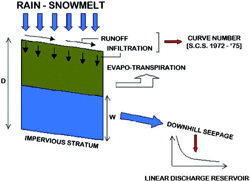
The reservoir is fed by the portion of the rain that infiltrates into the ground and emptied by subsurface flow and evapotranspiration Ev.

The rain that infiltrates into the ground is the rainfall height H(t), reduced by the run-off quantity R(t) which is calculated as follows:(3) where I_a is the initial abstraction, i.e. the initial rain height for which no run-off occur, usually assumed equal to 0.2S (USDA-SCS 1985, 1986).

The subsurface flow is described through an emptying function of the reservoir, ruled by an exponential function of λ, which is a discharge constant representative of the basin, as follows (Passalacqua 2002):(4)

The value of λ must be assessed according to the coefficient of hydraulic conductivity K_s, the slope gradient i and drainage length of the basin L, as(5) where K_s and i are parameters evaluated for each cell. The first one indicates the site permeability and is obtained reclassifying the land use map; the second one is simply calculated from the DTM. The drainage length of the basin L is a unique value for the whole basin, estimated performing a watershed analysis.

Given the emptying constant λ, the half-life time T_1/2, i.e. the time that the reservoirs employ to halve their own volume of water in the absence of supply, can be calculated as follows:(6)

The evapotranspiration of the vegetation covering the surface, Ev, is a factor difficult to evaluate, being a function of temperature, aspect and prevailing winds. In the present procedure mean daily values are automatically calculated depending on the daily average temperature observed in the site. For our case study, Ev values have a seasonally range between 10 and 15 mm/day in summer, and between 1 and 3 mm/day during winter.

The CN being a spatially distributed information, every cell is characterized by its own values of S, λ, T_1/2 and Ev. Moreover, the daily rainfall heights and temperatures are associated with each influence area, through the attribute table of the vector layer.

For any sequence of consecutive days of rainfall, according to the conditions of soil moisture due to the preceding four days’ rain history (as defined by the CN method), the IHG model calculates the water quantity that infiltrates into the ground H(t) − R(t) and its subsurface flow V(t+Δt). Hence, it allows determining:

• the oscillations of the phreatic table, with respect to its average level (previously assessed, if the site is characterized by a significant circulation even in the absence of rain as, for instance, when fed by perennial sources or snowy precipitations), and the actual volumes of infiltrating rain increasing the latter;

• the part of saturated soil.

2.3. The limit equilibrium conditions

Widespread slope stability analyses by a rather simplified global limit equilibrium method (Skempton & Delory 1957) are performed. This type of analysis is generally used when the following conditions occur:

• rupture surface (real or assumed) is formed by a plane (which often represents a discontinuity surface) which is approximately parallel to the slope;

• thickness of the layer involved in the landslide is small compared to the length of the landslide (you can then take the slope of infinite length, neglecting edge effects);

• the geomechanical properties of the soil and the pore pressure are constant along planes parallel to the ground level.

In this procedure, the method by Skempton & Delory (1957) is applied to each pixel of the model. Consequently the mass subject to landslide is not analysed by a single element (as in the method of infinite slope). Besides, since the cells can have different properties and conditions (from the geometrical, geotechnical and hydraulic standpoint) the shape of the whole 3D collapse surface can be irregular.

The implemented procedure allows the 3D assessment of local instability phenomena due to meteorological events. If many pluviometers are available, the rain history can be spatially varying.

For any rain history, the automatic calculation of the sliding safety factor for each cell is thus done by applying the equation (7).(7) where (see also figure 2)

Figure2. Cross section of the slope subjected to plane translational slide and identification of a vertical “slice” (the unit cell) of weight W.

F_S = sliding safety factor, c′ = soil's cohesion in effective stress terms, ϕ′ = soil's effective friction angle, z = cell's height, θ = inclination of the eventual slip surface, assumed as parallel to the ground surface, γ = unit weight of the soil, γ_w = unit weight of the water, and m = ratio between the saturated soil stratum and the element heights.

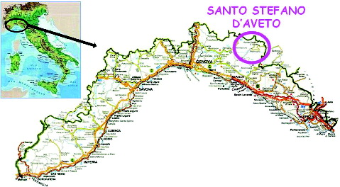
Figure3. The Santo Stefano d’Aveto site (Liguria, Italy).

It is worth recalling that the above-mentioned parameters are pertinent to each cell of the model.

The element height z is continuously increased until the bedrock level is reached, then the minimum obtained value of F_s is selected and this is assumed as the safety factor pertinent to that pixel unit. Consequently, for any rain history the safety factor is evaluated for each cell of the model, taking into account both the local features and parameters.

Finally, the results of the whole procedure are rendered in raster format, suitable even for not GIS expert users because of the immediacy of the map chromatic scale. The conversion from raster and vector data is always possible, for instance delimiting homogeneous areas.

3. A case study: the diffused and continuous kinematic phenomenon in Santo Stefano d’Aveto (Liguria, Italy)

The proposed procedure can be applied to any slipping site if well characterized from the hydrological and geotechnical points of view. In fact, information about the average level of the phreatic table and realistic values of the soils’ parameters has to be previously determined.

In the present research an extensive kinematic phenomenon surrounding the city of Santo Stefano d’Aveto (Italy) was examined, being this site strongly triggered by rainfall events and already interested by previous studies.

The sliding area is not limited to only one slope but it involves a region with complex morphology, composed by zones really affected by displacements or by areas influencing the neighbouring parts from the hydrological and geotechnical point of view.

3.1. Brief description of the site and phenomenon

A quite large area (∼5 km²) in the north-east sector of the Genoa province (see figure 3), which is part of the Liguria region (Northern Italy), is subjected to a complex and diffused kinematic phenomenon of sliding, not unanimously classified. A small town and six of its surrounding hamlets are located there. Normally almost 1250 inhabitants reside but, being this locality a well renown resort for both the winter and summer vacations, during a whole quarter of the year the residents’ number rises up to four times.

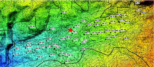
Figure4. Geophysical tests: 70 noise measurement points and one seismic array (red star) for the evaluation of the loose soil thickness.

The area of interest is sited on a top-valley gentle slope (mean dip angle 11°), which downgrades directly from the south-side faces of the Northern Apennines summits, locally arriving at 1800 m AMSL (above mean sea level). The entire area is classified as a large relict landslide, formed by a pliocenic glacial till and characterized by widely assorted sediments. The area, however, is affected by movements, so the above classification is improper. The main trigger actions on the soil body's behaviour are the seasonal rain/snow falls on the watershed. The soil heterogeneity and the correlated complicated hydrologic conditions of the zone induce significant relative displacements. Many buildings and generic structures (retaining walls, small bridges, etc.) exhibit damages, imputable to the widespread and locally differential movements at ground level. The state institutions, land authorities, as well as some of the private citizens, are applying their economical efforts in the rehabilitations and the assessment/control of the active phenomena.

Given the extension and complexity of the landslide, the use of a GIS-based platform is particularly indicated. It may integrate the DTM, the ground water and the bedrock layers. Moreover, the adoption of the automatic procedure, as described above, allows the analysis and prediction of instabilities triggered by rainfall events.

3.2. The 3D model

3.2.1. The loose soils’ thickness

From the geological and morphological points of view, the entire area was formed by a pliocenic glacial till and its body of widely assorted sediments had been classified as a large relict landslide, even if movements occur. The loose soils’ thickness spans from few meters up to 90, before of reaching the bedrock formations (argyllites, sandstones, mudstones, ophiolites and diabases in pillows).

Information about the subsoil has been deduced from:

• soil tests,

• data from boreholes, inclinometers and piezometers,

• seismic prospecting and MASW 2D.

Further information about the soil movements have been deduced by:

• traditional topography, GPS surveying and monitoring,

• synthetic aperture radar (SAR) interferometry.

The typical characterization techniques appear generally improper on such a wide scale and extremely variable loose soils’ deposit. Consequently, the authors have in this instance employed some non-conventional methods of deep-soundings and criteria of interpretation, in order to assess affordable but reliable site recognition over all its extension. Dealing with a rather large territorial dimension, one of the relevant issues is to find the proper techniques to spatially distribute the loose soils’ depth information, as well as the pertinent geotechnical parameters which, usually, are all gathered at spot locations but, as it is obvious, they are needed on the whole area in order to allow a widespread slope stability analysis approach. In the present analysis the geotechnical characteristics (unit weight of the soil, friction angle, cohesion and permeability) of the material involved were gathered only in three locations, then constant values were extrapolated for the whole area as a best guess. The availability of more information about the geotechnical characteristics, also in vertical direction, would improve the results obtained by the present procedure, which is able to consider complex sites.

Since the buried bedrock spatial morphology, depth and steepness have a key role on these sliding phenomena, a further characterization of the site geophysical tests have been performed. Noise measurements were made at more than 70 locations, placed on different parts of the loose soil body and of the surrounding exposed rock formations (see figure 4). Some of the recordings were carried out in proximity of those boreholes which had reached the bedrock depth, with the aim of assessing the shear velocity values of the glacial till materials. By using spectral ratio techniques, a good image of the resonance frequencies of the loose soil body was obtained. Moreover, one array set-up of six seismic stations allowed the study of the Rayleigh and Love wave dispersion.

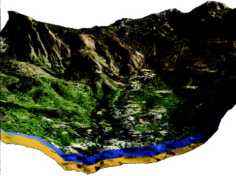
Figure5. The 3D GIS model; sections of the ground level, of the phreatic table (in blue) and of the bedrock (in yellow) are shown in the section at the lower part of the image, as three continuous surfaces.

Finally, the whole set of both the existing and the obtained data have been spatially distributed, by using standard interpolators available within the GIS platform. In particular, inverse distance weighted, regularized spline with tension and triangulated irregular network methods (respectively: r.surf.idw, r.surf.rst and r.surf.nnbathy commands in GRASS) were tested, searching the interpolator parameters in order to obtain the maximum accordance with measured data. The best performing method for this specific application was the triangulated irregular network one, by means of Delaunay algorithm.

3.2.2. The ground water

Since the subsurface water influence on the phenomenon is very important, the site was studied and tested from the hydrological point of view. The hydrological analysis of the site was divided into four phases.

The first one was carried out by a campaign of discharge measurements in the two rivers that through the glacial till longitudinally and join together downstream.

In the second one, the study of the superficial water flow in the rivers was based on a linear reservoir model, calibrating the pertinent parameters in accordance with the discharge measurements.

In the third phase, the model of the kinematic wave was used in order to define the steady groundwater level respecting the drainage in the riverbed and in the underground.

In the fourth and last one, the phreatic level oscillations were studied modelling each cell as an underground reservoir, as was described in Section 2.2.

Other methods could be used to estimate the position of the average phreatic level. It could be derived from the interpretation and interpolation of piezometric measurements, or via the present GIS procedure by analysing the evolution of the groundwater level triggered by a long-term (several years) rain history, until the configuration of stationary state is establishing.

3.2.3. The GIS platform

All the available and measured data were georeferenced and integrated into the GIS GRASS (ver. 6.4) platform, in order to examine the site. The spatial data had been thoroughly scrutinized, verified, assessed and assigned to different thematic layers.

The location was set up in the Gauss-Boaga cartographic projection and Rome40 reference system, coherent to the available regional technical cartography.

Additional and relevant information were added to the GIS platform, in the formof both raster and vector layers, such as the regional DTM, with resolution 5 m × 5 m, the land use map and the geo-lithological map, both at the scale 1:25,000, the reckoned landslides map at scale 1:10,000 and the results of a permanent scatterers’ interferometry analysis on SAR images (PSInSAR), which was yet performed by others (Gorziglia et al. 2008).

The steady distribution of the phreatic surface along the longitudinal axis of the glacial till, obtained as previously described, was extrapolated in the transversal direction through a Voronoi's tessellation.

From the loose soils’ thickness, computed by the shear wave velocities and the frequencies measured at spots (figure 4), a 3D model of its spatial distribution was created, selecting the most appropriate interpolation technique to obtain a reliable continuous description of the interface between loose soil and bedrock.

Consequently, the 3D model realized in GRASS contains three surfaces, corresponding to the DTM, the phreatic level and the bedrock (see figure 5).

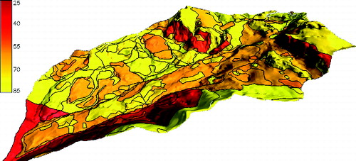
Figure6. 3D map showing the spatial variation of CN_II (low CN means low run-off and high infiltration).

3.3. Application of the procedure to the case study

The automatic procedure was applied to nine rainfall events of the past 7 years (see table 1). The analyses were made considering time windows 4 or 8 days long each, in which there had been a significant precipitation of rain. Periods characterized by not significant heights of rain were also analysed, in order to verify the reliability of the model.

Table1. Cumulative rainfall heights relative to the analysed events.

Year	Period	Time windows (days)	H (mm)
2003	27 October–3 November	8	249
2005	2–5 December	4	139
2006	14–17 August	4	111
2007	17–24 August	8	69
2007	21–24 November	4	228
2008	28–31 October	4	162
2008	9–16 December	8	152
2009	22–25 December	4	258
2010	31 October–3 November	4	196

Adopting the equations reported in Section 2.1, the spatial distribution of the CN was evaluated (an example is reported in figure 6). Then, the IHG model was applied to obtain the oscillations of the phreatic table (see figure 7), with respect to its steady level, and consequently the part of saturated soil. Finally, the attitude of the soil to slide as a result of meteorological events was analysed taking into account the local features. As final result of the procedure, a map of landslide susceptibility was automatically created (see figure 8), classifying the territory in function of the safety factor, defining as stable the zones characterized by F_s > 1.3 and as unstable the areas characterized by F_s < 1.0. The susceptibility to instability varies in function of the chromatic scale shown in figure 8. For any rain history, the calculation was performed on a total of 120,000 pixel units in 10 seconds.

Figure7. Map of the depth of the groundwater level, in metres with respect to the ground level, on the peak day of the analysed rainfall event occurred during November 2007.

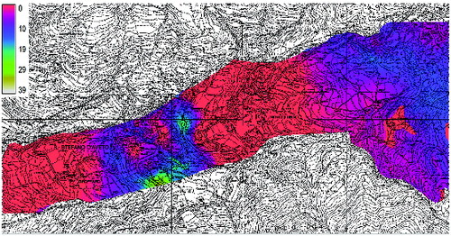
Figure8. Landslide susceptibility map relative to the analysed rainfall event occurred during November 2007; red and light green colours indicate high (F_s < 1) and low (F_s > 1.3) susceptibility, respectively.

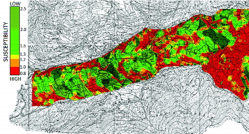
Figure9. Ground water levels measured in situ (at the yellow diamond) and calculated by the procedure (in metres below ground level); structural damages observed at the buildings highlighted in yellow.

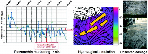
It is worth underlining that, in addition to the calculation of the ground water level at the end of the rain history, the model can also be used to observe its daily evolution, and thanks to the implementation in GIS, it can be represented for any desired cross-section.

Besides, the procedure is able to reproduce both localized and distributed variations of ground water table, depending on the type of rain history and on the period in which the rain occurs (temperature, conditions of initial moisture of the soil).

3.4. Validations of the results

As described above, the on-GIS implementation of the IHG method allows to obtain the groundwater's level variations, due to selected rain histories, and the spatially distributed susceptibility of the loose soils’ deposit to slide.

To validate the results obtained by the use of the implemented procedure, useful comparisons have been done. Some geotechnical and hydrological peculiarities were well detected.

The water pressure values deduced for the November 2007 rain history have been compared with the pertinent measured data. The obtained values of groundwater levels are in excellent agreement with piezometers’ recordings (see figure 9).

Figure10. Identification of Lake Riane (indicated by the red circle) in the half-time discharge map relative to the analysed rainfall event occurred during November 2007. The high values (in days) of half-time discharge enhance the high time necessary to the reservoirs to halve its volume of water in the absence of supply.

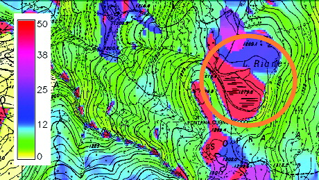
Moreover, analysing the processed results relating to the half-time discharge, the algorithm caught with marked accuracy the presence of a small vanishing lake. In figure 10 the high values of half-time discharge enhance the transient necessary to the reservoirs to halve their volume of water in the absence of supply. Such intermittent lake is indicated in cartography as Lake Riane and shows outcropping water very rarely, only when the rainfalls are significant.

Figure11. The PSInSAR rendering map (courtesy of Gorziglia et al.)

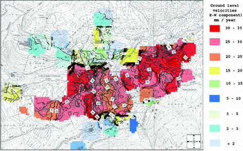
Besides, the IHG model's behaviour shows a good conceptual fit with the ground level's movements rendered by PSInSAR and by inclinometers, as can be seen in figures11 and 12. The comparison, although not strictly lawful, between zones with significant susceptibility to slide and high displacement areas, hints a qualitative reliability of the automatic procedure. A thorough site inspection showed that high significant structural damages were detected (both in recent and old structures, regardless of the type of structure and building material) in areas with high oscillations of groundwater level (see figure 13) and/or high susceptibility (see figure 14).

Figure12. Ground level displacements measured in a zone (indicated by the blue circle on the map which is relative to the analysed rainfall event occurred during November 2007), that lies downstream of an high susceptibility area.

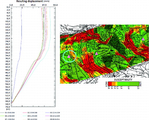
Figure13. Map of the average percentages of rising of groundwater level (relative to the analysed rainfall event occurred during November 2007) and images of structural damage in the castle and the leaning bell tower, as a result of ground displacements.

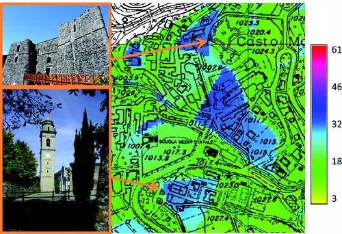
Figure14. Structural damages as seen on-site, caused by soil displacements, are in good agreement with the procedure results (relative to the analysed rainfall event occurred during November 2007).

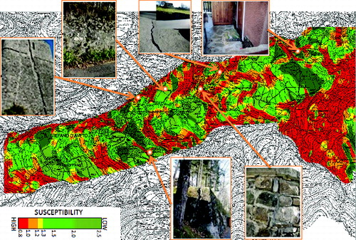
In figures 12–14, there are some inconsistencies. In fact, the on-site monitoring by inclinometers shows significant displacements in an area defined by the IHG model as not susceptible. Similarly, structural damages are sometimes in sites only next to areas characterized by high oscillations of groundwater level, or high susceptibility to instability. In this regard it is worth highlighting that in the automatic procedure the various cells of the model are considered to be non-interacting. In reality, areas of land may undergo displacements because they are involved by the movement of the ground surrounding them. The procedure could be improved, keeping this aspect into account. However, a correct interpretation of the created map already provides significant and promising indications. Concluding, such comparisons are effective in demonstrating that this procedure provides useful information on a wide area, taking into account the seasonal period and the rain histories.

4. Conclusions

In the present research, an automatic procedure in GIS was implemented in order to analyse the attitude to slide of widespread areas, considering the rainfall/snowmelt histories as the main triggering factor.

It can be applied to complex sites from the geometrical (e.g. any soil slope is analysable), geotechnical (e.g. parameters that vary in vertical and horizontal directions) and hydraulic (e.g. the water table level can vary from cell to cell) standpoint, because every cell can have different properties and conditions, and consequently the shape of the whole 3D collapse surface can be irregular.

The whole procedure is totally automatic and needs a low computational effort, producing maps of landslide susceptibility very quickly, allowing the modelling of temporally extended rain events (taking into account also the soil's moisture condition antecedent the event) and spatially extended area at a high resolution (e.g. 5 m).

In the present study, an extensive kinematic phenomenon surrounding the city of Santo Stefano d’Aveto was examined, as an interesting example of strong correlation between rainfall and soil's displacements. The IHG model results seem to be in excellent agreement with what is evident on site. Some geotechnical and hydrological peculiarities were well detected.

Note that this procedure can also be usefully and effectively applied to predict the hazard of instability scenarios, simply assuming synthetic histories of rainfall.

This work highlights on how the GIS may be a useful tool for the integration and analysis of georeferenced information in order to monitor, manage and plan the territory, also in support of risk analyses and mitigation.

In this sense, the fact that the procedure was implemented using a free and open source software might be of particular interest, in view of reuse and continuous improvement of the described tool.

In the near future, the authors will improve the IHG model considering for instance the interaction among the cells and more complex sliding phenomena.

Once the procedure is improved, appropriate comparisons with other methods (e.g. Xie et al. 2003; Montrasio & Valentino 2008; Marchesini et al. 2012) are already planned. Moreover, other sites will be studied in order to further validate the methodology.

Acknowledgements

The authors would like to thank Prof. Paolo Bartolini and Prof. Daniele Spallarossa, respectively, for the analysis of hydrological and geophysical investigations in Santo Stefano d’Aveto, as well as all of the graduating students who contributed to this research: a particular mention is due to Luca Terrile, who collaborated extensively to the latest developments. Moreover, we wish to thank the Settore Informativo Territoriale of Liguria Region, in the person of Lucia Pasetti, for having made available the layer mapping for the study area.

References

- Ayalew L, Yamagishi H. 2005. The application of GIS-based logistic regression for landslide susceptibility mapping in the Kakuda-Yahiko Mountains, Central Japan. Geomorphology. 65:15–31.
- Baum RL, Savage WZ, Godt JW. 2008. TRIGRS – A FORTRAN program for transient rainfall infiltration and grid-based regional slope-stability analysis, version 2.0. USGS Open-File Report 2008-1159, 75 p. Available from: http://landslides.usgs.gov/research/software.php
- Baum RL, Godt JW, Savage WZ. 2010. Estimating the timing and location of shallow rainfall-induced landslides using a model for transient, unsaturated infiltration. J Geophys Res. 115(F3):F03013. doi:10.1029/2009JF001321
- Bovolenta R, Federici B. 2010. Automatic procedure for landslide hazard mapping through GRASS. FOSS4G Conference, Barcelona, p. 1–6.
- Dahal RK, Hasegawa S, Nonomura S, Yamanaka M, Masuda T, Nishino K. 2008. GIS-based weights-of-evidence modelling of rainfall-induced landslides in small catchments for landslide susceptibility mapping. Environ Geol. 54(2):314–324.
- Garcia SG. 2002. A GIS GRASS-embedded decision support framework for flood forecasting. In: Proceedings of the Open source GIS-GRASS Users Conference 2002; September 11–13; Trento (Italy).
- Gorziglia G, Bottero D, Poggi F, Castello R, Minervini G. 2008. Final report on the Santo Stefano d’Aveto site surveys. Italian. Genoa (IT): Regione Liguria – Dipartimento Ambiente – Settore Assetto del Territorio.
- Guzzetti F, Carrarra A, Cardinali M, Reichenbach P. 1999. Landslide hazard evaluation: a review of current techniques and their application in a multi-scale study, Central Italy. Geomorphology. 31:181–216.
- Iverson RM. 2000. Landslide triggering by rain infiltration. Water Resour Res. 36(7):1897–1910.
- Lee S. 2007. Application and verification of fuzzy algebraic operators to landslide susceptibility mapping. Environ Geol. 52:615–623.
- Lu N, Godt J. 2008. Infinite slope stability under steady unsaturated seepage conditions. Water Resour Res. 44:W11404. doi:10.1029/2008WR006976
- Mancini R, Rosso R. 1989. Using GIS to assess spatial variability of SCS Curve Number at the basin scale. In: Kavas ML, editor. New directions for surface water modeling. IAHS Publication no. 181; p. 435–444.
- Maidment DR. 1993. GIS and hydrologic modeling. In: Goodchild MF, Parks BO, Steyaert, LT, editors. Environmental modeling with GIS. Oxford: Oxford University Press; p.147–167.
- Marchesini I, Cencetti C, De Rosa P. 2012. A preliminary method for the evaluation of the landslides volume at a regional scale. GeoInformatica. 13(3):277–289. doi:10.1007/s10707-008-0060-5
- Montgomery DR, Dietrich WE. 1994. A physically based model for the topographic control on shallow landsliding. Water Resour Res. 30(4):1153–1171.
- Montrasio L, Valentino R. 2008. A model for triggering mechanisms of shallow landslides. Nat Hazards Earth Syst Sci. 8:1149–1159. doi:10.5194/nhess-8-1149-2008
- Ohlmacher GC, Davis JC. 2003. Using multiple logistic regression and GIS technology to predict landslide hazard in northeast Kansa, USA. Eng Geol. 69:331–343.
- Passalacqua R. 2002. Vulnerabilità territoriale da frane e crolli in roccia [Spatial vulnerability to landslides and rock falls. Albenga (SV): Edizioni del Delfino Moro; p. 1–37. ISBN 88-88397-05-1. Italian.
- Passalacqua R, Baretto A. 2003. Landslides and rockfalls predictions by GIS in Western Liguria. In: Picarelli L, editor. Proceedings of the International Conference on Fast Slope Movements Prediction and Prevention for Risk Mitigation (FSM2003); 2003 May 11–13; Naples; p. 421–429. ISBN 8855526995.
- Passalacqua R, Bovolenta R, Spallarossa D, De Ferrari R. 2012. Geophysical site characterization for a large landslide 3-D modelling. In: Coutinho RQ, Mayne PW, editors. Proceedings of the 4th International Conference on Geotechnical and Geophysical Site Characterization, Porto de Galinhas, Brazil; 2012 Sept 17–21; London: Taylor & Francis Group (CRC Press – Balkema); p. 1765–1771. ISBN 978-0-415-62136-6.
- Passalacqua R, Bovolenta R. 2011. Integration of spatially distributed data for the 3D modelling of a kinematic phenomenon in Italy. In Proceedings of the IAMG (International Association for Mathematical Geosciences) 2011 Conference; Austria: University of Salzburg; p. 111–119. doi:10.5242/iamg.2011.0185
- Pradhan B, Lee S. 2010. Regional landslide susceptibility analysis using back-propagation neural network model at Cameron Highland, Malaysia. Landslides. 7:13–30.
- Qiu C, Esaki T, Xie M, Mitani Y, Wang C. 2007. Spatio-temporal estimation of shallow landslide hazard triggered by rainfall using a three-dimensional model. Environ Geol. 52:1569–1579.
- Skempton AW, Delory FA. 1957. Stability of natural slopes in London Clay. In Proceedings of 4th International Conference on Soil Mechanics; London (UK); Vol. 2; p.378–381.
- [USDA-SCS] US Department of Agriculture Soil Conservation Service. 1985. National engineeringhandbook: Section 4 – Hydrology (NEH-4). Washington (DC): US Department of Agriculture.
- [USDA-SCS] US Department of Agriculture Soil Conservation Service. 1986. Urban hydrology for small watersheds. Technical Release No. 55 (TR-55). 2nd ed. Washington (DC): US Department of Agriculture.
- Wu W, Sidle RC. 1995. A distributed slope stability model for steep forested basins. Water Resour Res. 31(8):2097–2110.
- Xie M, Esaki T, Zhou G, Mitani Y. 2003. Geographic information systems-based three-dimensional critical slope stability analysis and landslide hazard assessment. J Geotech Geoenviron Eng. 129(12):1109–1118.