Simulating land use change by integrating ANN-CA model and landscape pattern indices

Abstract

Artificial neural network–cellular automata model has been applied successfully in land use change simulation. However, it has rarely been integrated with landscape pattern indices (LPIs), the embodiment of the spatial heterogeneity of land use. This paper proposed to integrate LPIs as the parameters of artificial neural network–cellular automata model. Subsequent to a description of the principles and implementation of the model, a case study was presented in Changping district. In the case study, two LPIs, the landscape similarity index and patch density, along with 10 other spatial variables, were selected as the influencing factors of land use change. Based on land use maps in years 1988 and 1998, a land use map in 2008 was simulated by the proposed model. Comparing with the actual land use map in 2008 and the simulated result of artificial neural network–cellular automata model, the results showed that the proposed model is more applicable for simulating land use change in the study area; the limitation of this model is the spatial scale and calculation method of LPIs.

1. Introduction

Simulation of land use change (LUC) provides a new approach to support the planning and management of land use. However, LUC is a complex process, which would be driven by a series of natural and social factors. Also, the drivers operate across a variety of spatial–temporal scales in a nonlinear way. Modelling LUC simulation systems is challenging. Therefore, advanced approaches are required (Tayyebi et al. 2014a, 2014b).

Artificial neural networks–cellular automata (ANN-CA) model, a nonlinear tool, has been applied successfully in LUC simulation (Mahajan & Venkatachalam 2009; Pijanowski et al. 2014). In the model, CA performs as a bottom-up simulation framework. ANN is used as data mining tools to mine the transition rules of LUC for CA; it means that ANN is used to understand the underlying patterns in LUC data. ANN has the advantage of being able to observe relationships in data by emulating the brain's ability to sort patterns through the interconnected systems of many neurons (Arekhi & Jafarzadeh 2014; Tayyebi & Pijanowski 2014). ANN is an appropriate global parametric model for simulating LUC whereas various spatial drivers simulate land transformation in a non-linear way. Also, ANN is very effective in handling incorrect and inferior data, and capturing non-linear, complex features in modelling processes; therefore, it has been generally accepted that they are capable of achieving results with superior accuracy in modelling (Li & Yeh 2002). Tayyebi et al. (2014b, 2014c) compared the land transformation models based on ANN, classification, and regression tree, and multivariate adaptive regression spline model, and proved the advantage of ANN than other models in both temporal and spatial accuracies.

There are few studies that use ANN-CA model to simulate LUC; however, in the former research works, the landscape pattern indices (LPIs) have not been integrated into the ANN-CA model. LPIs, the embodiment of the spatial heterogeneity of land use, were often used for describing the LUC (Seto & Fragkias 2005; Serra et al. 2008; Liu et al. 2010; Feng et al. 2011). Researches have shown that LPIs can influence a variety of ecological phenomena. Recently, they have been researched as influence factors of urban expansion and LUC (Zeng et al. 2004; Mitsuda & Ito 2011). Also, researchers have started to attempt to integrate LPIs into urban expansion simulation model and LUC simulation model (Liu et al. 2014; Li et al. 2013; Yang et al. 2014).

Liu et al. (2014) build an urban expansion simulation model by integrating LPIs and CBR (case-based reasoning)-CA. A particular LPI, landscape expansion index (LEI, an index designed based on LPIs) was used to identify the growth type to influence the cellular evolution. In contrast with traditional LPIs which only reflect the spatial characteristics at a given time, LEI can capture the information on formation processes of a landscape pattern. LEI was calculated for each cell, which could help identify urban growth type, and then got different transition rules for different growth types. Li et al. (2013) build an urban expansion simulation model by integrating LPIs and GA (genetic algorithm)-CA. They attempted to calibrate urban expansion simulation models according to the LPIs of the whole study area. Their model uses a fitness function based on LPIs to affect the weights of urban expansion factors, which are generated by GAs. Put simply, it controls the urban expansion by controlling the landscape pattern of the whole study area. Yang et al. (2014) have attempted to build an LUC model by integrating LPIs with Markov-CA model (Markov-CA-LPIs). In the model, relationships between un-transition probabilities and LPIs of land use types in different sub-regions among the study area are discovered, and then used to generate un-transition probability maps, which are used as suitability maps of Markov-CA model. In this integrating way, the last transition probabilities of LUC are dependent on the transition probabilities calculated by LPIs and the transition probabilities calculated by some other variables.

In this paper, an ANN-CA-LPIs simulation model, integrating LPIs into ANN-CA model, was proposed. This model also tries to differentiate the transition probabilities of land use in different spatial regions of study area through a different landscape pattern, which is the same as Markov-CA-LPIs model. However, different from the Markov-CA-LPIs model, in the model proposed by this paper, the last transition probabilities of LUC are dependent on the transition probabilities calculated by LPIs and other variables.

To demonstrate the feasibility and advantage of the model, a case study of the Changping district in Beijing is presented. The paper is organized as follows: Section 2 presents a description of LPIs, explains the architecture of the ANN-CA model, and describes the integration of LPIs and ANN-CA model. Section 3 presents the case study. In Section 4, conclusion and outlook for the future are presented.

2. Landscape pattern indices

LPIs are quantitative descriptions of landscape patterns (Hu & Dong 2013). Landscape patterns are distinguished by spatial relationships among component parts, and can be characterized by both composition and configuration. Landscape composition refers to features associated with the presence and amount of each patch type within the landscape, but without being spatially explicit. Landscape configuration refers to the physical distribution or spatial character of patches within the landscape.

There are various indices for describing landscape patterns quantitatively (McGarigal & Cushman 2002). If all of them were chosen to be integrated into the LUC simulation model, the simulation process must be very complicated. Taking the former research as the reference, in this paper, the landscape similarity index (LSI) and patch density (PD) at class level were chosen to be integrated into the LUC model.

The LSI at class level represents the per cent of the landscape occupied by the class. It is an index to quantify the landscape composition. It was chosen because the LUC of a patch could be influenced by the abundance of patches of the same land use type in the surrounding landscape. A patch with a high LSI for land use types in the landscape may be more difficult to change to other land use types. This index is calculated as follows: (1) where i represents the patch types (land use classes); j represents the number of patches; n is the total number of patches; a_ij is the area (m² ) of patch ij; A is the total landscape area (m²); and LSI_i is the landscape similarity index of the land use class i.

PD is a fundamental index that represents the landscape configuration. It expresses the number of patches per unit within an area, and best describes landscape fragmentation. Holding the total area constant, a landscape with a greater density would be considered more fragmented than a landscape with a lower density. A land use type with a high PD in the landscape may be easier to change to another land use type. This index is calculated as follows: (2) where PD_i is the patch density of land use class i and n is the total number of patches.

The LPIs could be calculated using FRAGSTATS, which is an outstanding software developed to quantify landscape structure (Liu et al. 2010).

3. Integrating LPIs into ANN-CA model

ANN-CA model has been applied widely in LUC change simulation, and in those literatures, the ANN-CA model was described in detail. In this section, after a brief introduction of the ANN-CA model, the integration of LPIs with ANN-CA model is introduced.

In an ANN-CA model, the CA provides a spatio-temporal framework for LUC simulation; ANN is applied to discover the local transition rules of CA (Li & Yeh 2002; Lin et al. 2011). In the input layer of ANN, neurons are a set of cellular attributes, which are social, economic, and physical factors. It was assumed that these attributes determined the LUC probabilities. A neuron in the output layer of ANN corresponds to a land use class. The value of a neuron in the output layer represented the transition probability from the existing class to the corresponding land use class.

In this paper, LPIs were incorporated as attributes, which are set as neurons in the input layer of ANN to determine the LUC probabilities. Therefore, transition probability of land use class is conducted by LPIs and other conditions together. The probability of LUC is designed as follows: (3) where P_LUC is the probability of LUC; is a probability calculated by a function consisting of LPIs, Other conditions, and a set weight generated from ANN. In ANN, the function is non-linear and hidden. Other conditions are mentioned as the social, economic, and physical factors of LUC.

The integrating way of LPIs with ANN-CA is absolutely different from the way in Markov-CA-LPIs. In Markov-CA-LPIs model, the transition probability maps conducted by LPIs are similar to the suitability maps, and LUCs are determined by the value of suitability. In the Markov-CA-LPIs model, the transition probability of land use class is conducted by the probability conducted by LPIs and the probability conducted by other conditions. The probability of LUC can be described as follows: (4) where P_LPIs is the probability of LUC conducted by LPIs; is the probability of LUC conducted by the other conditions; and is the minimum value between P_LPIs and .

Combined with the above description, the structure of the ANN-CA model could be described as shown in figure 1. There is a problem that LPIs are the characteristics of a land use class, but the attributes in the input layer of ANN are the characteristic of a cell. To solve the problem, the LPIs must be transformed to the characteristic of a cell. Therefore, in this paper, LPIs of a cell were set as the LPIs of the cellular land use class in a certain landscape.

Figure 1. Processing architecture of ANN-CA model coupling with LPIs.

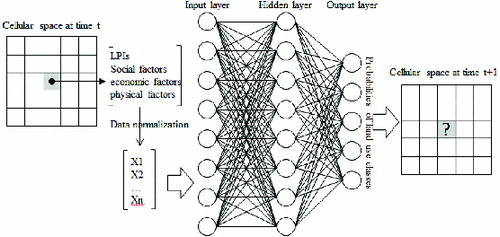
In the simulation process, the LUC of a cell was determined by comparing the values of transition probabilities generated by neurons in the output layer. Land use class would transit to the class that is associated with the highest value of transition probability. If the classes have the same highest transition probability, randomness could be generated to make the decision.

The simulation of LUC was carried out by running CA and an ANN for a sufficient number of steps. Whether a cell is converted or not is usually decided by many steps of evolution. To control the rate of LUC in one step, a predefined threshold (ranged from 0 to 1) should be set. In this paper, a relative large value of 0.9 was defined as the threshold. It was proved that this value is useful for obtaining the fine simulation patterns, which can prevent land use from changing too fast.

4. Implementation of the model

To demonstrate the feasibility of ANN-CA-LPIs model, it was implemented to simulate LUC in the Changping district (with an area of 1352 km²), Beijing, China. This district was selected as a study area because of its significant spatial differences in the landscape patterns and the data availability. As some of its edges comprised the outer borders of the central area of Beijing, Changping is a rapidly growing area. While it was undergoing rapid economic development, the land use changed dramatically under the influence of human environmental systems.

4.1. Data sources

The data used to provide actual urban areas for this case study included three land use maps generated from the classifications of Landsat TM5 images, acquired during the summers of 1988, 1998, and 2008, at a spatial resolution of 30 m. Each land use map was treated as a cellular space, with each pixel representing a cell. Thus, each cell represents an area of 30 × 30 m, or 900 m². The maps contained five land use/land cover classes: forest land (FL), cultivated land (CuL), construction land (CoL), water (WL), and other land uses (OLU). The two maps for 1988 and 1998 were used to capture the transition rules. The 2008 map was used to test the simulation result.

In this paper, in addition to the two LPIs, a total of 10 spatial variables were used for the attributions of the cells. Table 1 lists the details of the spatial variables. They included a series of distance-based variables, neighbourhood conditions, and physical attributes, which could be derived from remote sensing and GIS data. Studies have shown that these variables are closely related to the probability of LUC. In this paper, social and economic variables were not chosen as the attributions of the cells because the fine resolution census data at early in Changping are rarely available.

Table 1. Spatial variables used for the conditional items of local transition rules.

	Spatial variable	Short name
Physical attribute	Cellular initial state	IS
	Distance from the cell to the major urban areas	Dist(MU)
	Distance from the cell to the closest town areas	Dist(CT)
Distance-based variables	Distance from the cell to the closest road	Dist(CR)
	Distance from the cell to the closet railway	Dist(CW)
	Amount of cells used as forest	Num(FL)
	Amount of cells used as cultivated land	Num(CuL)
Neighbourhood conditions	Amount of cells used as construction land	Num(CoL)
	Amount of cells whose states are water	Num(WL)
	Amount of cells used as other unused land	Num(OLU)

To derive the distance-based variables, traffic data were prepared from urban and town areas (in GIS format) from the years 1988 and 1998. The Euclidean distance function of ArcMap was used to obtain the Euclidean distance raster map for the distance-based variables.

To derive the neighbourhood conditions, a standard 7 × 7 contiguity filter was used. Other types of contiguity filters could be used; however, an earlier research (Pan et al. 2010) indicated that a combination of small cell sizes and small neighbourhood sizes generated improper expressions of land use transitions.

4.2. Analysis of LPIs and LUC

An analysis of LPIs and LUC of different spatial sub-regions in Changping from 1988 to 1998 was performed. The analysis about the differences of LUC and LPIs among different sub-regions may be helpful for examining the viability of simulating LUC integrating with LPIs. To realize the analysis well, 12 sub-regions were extracted from the maps using the Extract by Mask tool in ArcGIS. The sub-regions are clearly with different landscape patterns.

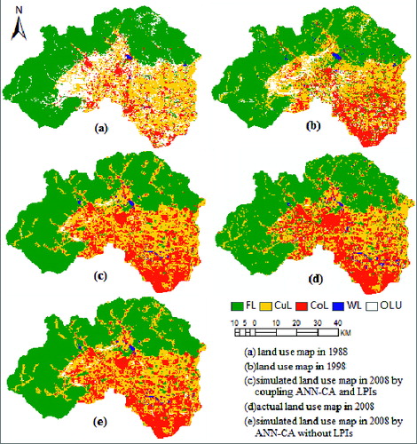
First, the LUCs from 1988 to 1998 in the whole Changping district were calculated. The land use maps in 1988 and 1998 were shown in figure 2(a) and 2 (b). Using the CROSSTAB model in IDRISI, LUCs were obtained and shown in table 2. Then, the LUCs of the 12 sub-regions in Changping from 1988 to 1998 were calculated. Using the CROSSTAB model in IDRISI, LUCs in those sub-regions were obtained and shown in table 3. From table 3, it can be seen that changes in the area of each land use class among those sub-regions had great differences. The change ratios of the sub-regions and the entire Changping district also had great differences. Finally, LSI and PD of the sub-regions were calculated using the software FRAGSTATS (table 4).

Table 2. Changes in land use area in Changping, 1988–1998^a.

	FL	CuL	CoL	WL	OLU
1988 (km^2)	671.93	313.38	121.34	2.87	242.48
1998 (km^2)	680.81	367.28	206.46	5.83	91.62
Changed area (km^2)	8.88	53.9	85.11	2.96	−150.85
Change ratio (%)	0.657	3.987	6.295	0.219	−11.158

^aThe change ratio is the percentage of changed area in the study area.

Table 3. Change ratios (%) in land use area in the sub-regions of Changping, 1988–1998^b.

No. of sub-regions	FL	CuL	CoL	WL	OLU
1	0.418	1.770	0.055	−0.405	−1.838
2	20.980	3.878	−23.131	0.132	−1.858
3	8.466	14.319	−18.997	−0.142	−3.646
4	22.774	18.266	14.594	−0.115	−55.519
5	6.312	0.492	19.452	−2.274	−23.982
6	15.610	17.471	−26.001	2.415	−9.495
7	−8.002	24.259	10.544	−0.086	−26.716
8	2.009	9.384	2.783	−0.178	−13.998
9	5.814	3.351	−5.016	0.379	−4.528
10	16.013	−0.318	1.616	−0.041	−17.269
11	25.261	10.148	−0.399	−1.600	−33.410
12	27.773	2.403	−4.901	−1.125	−24.149

^bThe change ratio is the percentage of changed area in the sub-region.

Table 4. LPIs in 12 sub-regions of Changping in 1988.

	FL		CuL		CoL		WL		OLU
No. of sub-regions	LSI	PD	LSI	PD	LSI	PD	LSI	PD	LSI	PD
1	97.498	0.184	0.204	0.398	0.055	0.061	0.405	0.031	1.838	2.018
2	5.283	11.998	46.020	3.321	39.983	2.035	0.024	0.030	8.690	4.428
3	2.790	6.174	13.315	2.736	52.750	0.430	0.106	0.091	5.966	2.556
4	13.158	10.939	10.846	3.463	12.479	3.384	0.480	0.126	63.037	1.212
5	7.602	13.929	30.302	4.485	30.160	2.725	2.664	0.246	29.273	3.785
6	8.078	14.251	30.740	6.111	48.765	1.667	0.202	0.169	12.215	4.299
7	44.336	6.330	7.547	1.427	10.679	2.488	0.086	0.220	37.352	1.976
8	84.662	0.879	0.211	0.381	0.137	0.117	0.178	0.322	14.812	1.904
9	1.918	4.487	14.214	1.926	35.340	0.618	0.038	0.076	5.168	2.307
10	68.944	2.200	4.440	2.389	0.311	0.177	3.387	0.286	17.313	2.718
11	38.566	8.018	12.830	4.627	9.767	2.589	1.125	0.177	35.449	2.417
12	23.420	10.088	32.842	3.196	15.042	2.297	0.405	0.031	27.570	3.726

Figure 2. Land use maps. (a), (b) and (d) reprinted from Ecological Modelling, Vol. 233, X. Yang, X.Q. Zheng and L.N. Lv, A spatiotemporal model of land use change based on ant colony optimization, Markov chain and cellular automata, pp. 11-19. Copyright 2012, with permission from Elsevier. To view this figure in colour, please see the online version of the journal.

From tables 3 and 4, we can see that similar to LUC, LPIs among the sub-regions had great differences too. It is difficult to obtain quantitative conclusions by observing data of LUCs and LPIs, and no attempt was made to quantify the relationship between the LUCs and LPIs, or to measure their strength. A conclusion was reached that LUCs in the regions with different landscape patterns were also different.

4.3. Simulation process

The 10 spatial variables of a cell, listed in table 1, were easy to obtain. The determination of the LPIs for the cells, however, was a problem. As mentioned in Section 2.2, the LPIs of a cell were set as LPIs of the cellular land use class within a specific region; therefore, the calculation of the LPIs first required the determination of a spatial region for a cell. It was unwise to generate a sub-region for each cell (the sub-region takes the corresponding cell as its centre), and calculate the LPIs of those sub-regions. Although this method was impartial to all the cells, the LPIs of each cell obtained by this method could best represent the characteristics of the spatial environment in which it was located. This would require very sizeable calculations.

In order to simplify the calculations, the Changping district was divided into 12 sub-regions, of four equal longitudinal sections, and three equal latitudinal sections. Through visual observations, landscape patterns from the sub-regions in 1988 displayed great differences, and again in 1998, they also displayed significant differences. Using the software FRAGSTATS, LPIs (LSI and PD) were calculated at class levels of the 12 sub-regions in both 1988 and 1998. The LPIs of a sub-region were set as the LPIs values of the cells, which are in located in the sub-region.

After preparing data, training the ANN was essential before the simulation using the ANN-CA model. The data from 1988 to 1998 were used to train the ANN and obtain the transition rule for the CA. It was unwise to use the whole data-set for training, because the data volume was so large. A total of 50,000 random samples (about 33% of all cells) were proportionally selected from the different land use classes, and they were evenly distributed within 12 sub-regions. There were a total of 12 variables for each cell, and consequentially, there were 12 neurons in the input layer. The number of neurons within the hidden layer was also set as 12. The number of land use classes decided the number of neurons in the output layer. So there were 5 neurons in the output layer. No explicit transition rules were required for an ANN-CA model. The only task was to train the neural network to obtain parameter values based on empirical data.

After training the ANN using the 50,000 samples, setting the LPIs and the spatial variables in 1998 as neurons in input layer of ANN, the ANN could then be used to generate the transition probabilities of cells from 1998 to 2008, which were provided for CA to simulate the land use map in the year 2008.

4.4. Results and discussion

The simulated land use map in 2008 was generated, and was shown in figure 2 (c). In order to analyse the simulated result, it should be compared with the actual land use map in 2008, which is shown in figure 2(d).

Visual comparisons with the actual land use map indicated that FL, CuL, CoL, and WL in the simulated map were relatively close to the corresponding classes in the actual map. The greatest agreement was shown in the FL in the north of Changping. The main deviations were located in the central area, where there were much greater OLU and CuL, and a lesser amount of CoL in simulated map.

Then, quantitative comparison was carried out to analyse the accuracy of the simulation results. The simulated areas, the actual areas, the simulated changed ratio from 1998 to 2008, the actual changed ratio from 1998 to 2008, and the error rates, counted by categories, were listed in table 5. The CROSSTAB model in IDRISI was then used to obtain the Kappa Index of Agreement (KIA) with the actual land use map as reference. KIAs were also listed by categories in table 5.

Table 5. Comparison of accuracy for simulated area by coupling ANN-CA and LPIs and actual area.

	Simulated area (km^2)	Actual area (km^2)	Simulated changed ratio (%)	Actual changed ratio (%)	Error rate	KIA
FL	674.38	666.75	−0.944	−2.065	0.0114	0.761
CuL	383.65	354.01	4.457	−3.613	0.0837	0.582
CoL	255.64	316.11	23.821	53.110	−0.1913	0.497
WL	8.56	10.73	46.827	84.048	−0.2022	0.372
OLU	29.77	4.39	−67.507	−95.209	5.7813	0.084

In terms of quantitative accuracy, error rates for FL and CuL were particularly low at −0.0114 and 0.0837, respectively. Comparing the simulated changed ratios and actual changed ratios, we can see that (1) for the simulated result, the area of land use classes except FL and OLU was expanded. However, actually, only CoL and WL were expanded; the area of CuL was decreased. (2) The actual decrease speeds of FL and OLU were faster than the simulated decrease speed, and the actual expansion speed of CoL was also faster than the simulated expansion speed. Those are caused by using transition rules from 1988 to 1998 to simulate the transitions from 1998 to 2008; however, the urbanization from 1998 to 2008 was more intensive than urbanization from 1988 to 1998. In terms of the spatial accuracy, the KIAs for FL, CuL, CoL, and WL are at 0.761, 0.582, 0.497, and 0.372, respectively. This means the accuracy of the spatial distributions was acceptable.

The results showed that the accuracies of the quantity and spatial distributions were both acceptable. Therefore, the simulation accuracies were acceptable. This indicated that the ANN-CA-LPIs model could simulate future land use patterns objectively and accurately.

4.5. Model validation and comparison

In order to validate the advantage of integrating LPIs into the ANN-CA model, the result simulated by ANN-CA-LPIs was compared with the result simulated by ANN-CA model without integrating LPIs. The spatial variables other than the LPIs, as parameters of local transition rules used in the ANN-CA model, were the same as those used in the ANN-CA-LPIs. The map simulated by the ANN-CA model was shown in figure 2(e).

To compare the results quantitatively, the simulated results, the error rate, and the KIA of the ANN-CA model were listed by categories in table 6, from which it could be seen that the error rates of the ANN-CA model were close to the error rates of the ANN-CA-LPIs model. This demonstrates that in terms of the total amount of land use, the two models also showed high accuracies. In terms of the spatial accuracy of the ANN-CA model, the KIAs for FL, CuL, and WL were at 0.714, 0.536, and 0.398, respectively, which were lower than those of the ANN-CA-LPIs model. The KIA for the CoL of the ANN-CA model was slightly higher than that of the ANN-CA-LPIs model. The KIAs for the OLU of the ANN-CA and ANN-CA-LPIs models were both very low.

Table 6. Simulation result of ANN-CA model without LPIs.

	Simulated area (km^2)	Error rate	KIA
FL	674.41	0.0114	0.714
CuL	383.59	0.0836	0.536
CoL	255.65	−0.1912	0.499
WL	8.55	−0.2032	0.398
OLU	29.79	5.7859	0.041

Further discussions of the quantitative analysis result were carried out through visual comparison. Using the crosstab map generated from the analysis of CROSSTAB, error maps, non-match maps and match maps between the simulation results, and actual map in 2008 were obtained, as shown in figures 3 and 4.

Figure 3. Error maps and non-match maps of simulation results conducted by the two models. The two sub-figures (ALL, ANN-CA-LPIs) and (ALL, ANN-CA) are non-match maps; cells in (ALL, ANN-CA-LPIs) mean that they have different land use classes in map simulated by ANN-CA-LPIs and actual map in 2008; cells in (ALL, ANN-CA) mean that they have different land use classes in map simulated by ANN-CA and actual map in 2008. The other sub-figures are error maps; those error maps are defined as follows: taking (FL, ANN-CA-LPIs) as example, land use class of the cells in the error map is FL in actual map of 2008, but they are not FL in the map simulated by ANN-CA-LPIs.

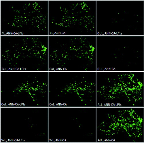
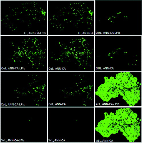
Figure 4. Error maps and match maps of simulation results conducted by the two models. The two sub-figures (ALL, ANN-CA-LPIs) and (ALL, ANN-CA) are match maps; cells in (ALL, ANN-CA-LPIs) mean that they have the same land use classes in map simulated by ANN-CA-LPIs as actual map in 2008; cells in (ALL, ANN-CA) mean that they have the same land use classes in map simulated by ANN-CA as actual map. The other sub-figures are error maps; definitions of those error maps are different from figure 3; they are defined as follow: taking (FL, ANN-CA-LPIs) as example, land use class of the cells in the error map is simulated as FL, but in the actual map, they are not FL.

In figure 3, the two sub-figures (ALL, ANN-CA-LPIs) and (ALL, ANN-CA) are non-match maps; cells in (ALL, ANN-CA-LPIs) mean that they have different land use classes in map simulated by ANN-CA-LPIs and actual map in 2008; cells in (ALL, ANN-CA) mean that they have different land use classes in map simulated by ANN-CA and actual map in 2008. The other sub-figures are error maps; those error maps are defined as follows: taking (FL, ANN-CA-LPIs) as example, land use class of the cells in the error map is FL in actual map of 2008, but they are not FL in the map simulated by ANN-CA-LPIs.

In figure 4, the two sub-figures (ALL, ANN-CA-LPIs) and (ALL, ANN-CA) are match maps; cells in (ALL, ANN-CA-LPIs) mean that they have the same land use classes in map simulated by ANN-CA-LPIs as actual map in 2008; cells in (ALL, ANN-CA) mean that they have the same land use classes in map simulated by ANN-CA as actual map. The other sub-figures are error maps; definitions of those error maps are different from figure 3; they are defined as follows: taking (FL, ANN-CA-LPIs) as example, land use class of the cells in the error map is simulated as FL, but in the actual map, they are not FL.

From error maps, non-match maps, and match maps, simulation characteristic of the two models can be obtained conveniently. Error maps in figure 3 implied that in simulation models, conditions of the cells in those map in year 1998 were difficult for them to transit to or maintain the corresponding land use class. Error maps in figure 4 implied that in simulation models, conditions of the cells in those map in year 1998 were easy for them to transit to or maintain the corresponding land use class. There exist some differences between error maps in figure 3. However, it seems not easy to detect the difference between the two models from figure 3.

The most obvious differences exist between the OLU error maps in figure 4. In the map simulated by the ANN-CA model, there were still some OLU in the east of Changping that did not transited; but in the map simulated by the ANN-CA-LPIs model, the OLU in the east of Changping did completely transited, which was closer to the actual situation. In the east of Changping, the transition probabilities of OLU in the ANN-CA-LPIs model were greater than those in the ANN-CA model.

Other obvious differences exist between the FL error maps in figure 4. In the southeast of Changping, the FL in the simulated map of the ANN-CA model was obviously larger than the FL in the simulated map of the ANN-CA-LPIs model. In the southeast of Changping, the transition probabilities of the FL in the ANN-CA model were smaller than those from the ANN-CA-LPIs model.

The other differences exist between the CuL error maps in figure 4. In the southwest of Changping, the CuL in the simulated map of the ANN-CA model was obviously larger than the CuL in the simulated map of the ANN-CA-LPIs model. In the southwest of Changping, the transition probabilities of the FL in the ANN-CA model were smaller than those from the ANN-CA-LPIs model.

For the other two land use classes, (1) the areas of WL were small, and therefore, the differences between the results simulated by the two models were slight; (2) although KIA of FL in the map simulated by ANN-CA model is higher than ANN-CA-LPIs model, there were no obvious differences between the error maps of FL in figure 4. It seems that the integration of LPIs did not achieve good result for WL and CoL.

Overall, combining the quantitative accuracy and the spatial accuracy, the model proposed by this paper has much better simulation performance. With the same spatial variable restrictions, this model enhanced the ANN-CA model by improving the spatial accuracy through the use of LPIs to restrict spatial distribution.

5. Conclusion

This paper proposed to integrate LPIs into ANN-CA while simulate LUC. LPIs, a useful quantitative measure for describing the structures and patterns of a landscape, could be used to quantify spatial heterogeneity and to reflect important spatial properties. These indices provide important information that can characterize urban and land-use systems. They have been applied in the areas of the detection of LUC, urban expansion, biodiversity, and habitat fragmentation.

In this paper, two LPIs, the landscape similarity index and patch density, were selected to be integrated into the ANN-CA model. Also, the model was applied to simulate LUC in Changping, China. To simplify the calculations of LPIs, the Changping district was divided into 12 sub-regions, of four equal longitudinal sections and three equal latitudinal sections; cells with the same land use class in the same sub-region have the same LPIs. The experimental results indicated that the simulation accuracies of this model were superior to the accuracies of an ANN-CA model. That was achieved through differentiating the transition probabilities of land use in different spatial regions of study area through the different landscape pattern.

Although the proposed method can yield reasonable simulation results, it was subject to some limitations. One limitation was the spatial scale of the LPIs. In this study, the Changping district was simply divided into 12 small sub-regions. Another limitation was the calculation method of LPIs, which is impartial for some cells. For example, the cells in the boundary area of a sub-region showed landscape pattern conditions that were the same as the cells in the centre of the sub-region, which is obviously inaccurate and counterproductive for improving the simulation accuracy. The accuracies of some land use classes (e.g. KIA of FL) may be restricted by those limitations. These problems will need to be addressed in further research.

Additional information

Funding

This research was supported by the National Key Technology R&D Program [grant number 2012BAK27B02]; China Postdoctoral Science Foundation [grant number 2014M560120]; and National Public Benefit Research Foundation of China [grant number 201310118].

References

- Arekhi S, Jafarzadeh AA. 2014. Forecasting areas vulnerable to forest conversion using artificial neural network and GIS (case study: northern Ilam forests, Ilam province, Iran). Arab J Geosci. 7:1073–1085.
- Feng Y, Luo G, Lu L, Zhou D, Han Q, Xu W, Yin C, Zhu L, Dai L, Li Y, et al. 2011. Effects of land use change on landscape pattern of the Manas River watershed in Xinjiang, China. Environ Earth Sci. 64:2067–2077.
- Hu R, Dong S. 2013. Land use dynamics and landscape patterns in Shanghai, Jiangsu and Zhejiang. J Resour Ecol. 4:141–148.
- Li X, Lin J, Chen Y, Liu X, Ai B. 2013. Calibrating cellular automata based on landscape metrics by using genetic algorithms. Int J Geogr Inf Sci. 27:594–613.
- Li X, Yeh AG. 2002. Neural-network-based cellular automata for simulating multiple land use changes using GIS. Int J Geogr Inf Sci. 16:323–343.
- Lin YP, Chu HJ, Wu CF, Verburg PH. 2011. Predictive ability of logistic regression, auto-logistic regression and neural network models in empirical land-use change modeling – a case study. Int J Geogr Inf Sci. 25:65–87.
- Liu X, Li X, Chen Y, Tan Z, Li S, Ai B. 2010. A new landscape index for quantifying urban expansion using multi-temporal remotely sensed data. Landsc Ecol. 25:671–682.
- Liu X, Ma L, Li X, Ai B, Li S, He Z. 2014. Simulating urban growth by integrating landscape expansion index (LEI) and cellular automata. Int J Geogr Inf Sci. Jan 2; 28:148–163.
- Mahajan Y, Venkatachalam P. 2009. Neural network based cellular automata model for dynamic spatial modeling in GIS. International Conference on Computational Science and its Applications; Seoul.
- McGarigal K, Cushman SA. 2002. Comparative evaluation of experimental approaches to the study of habitat fragmentation effects. Ecol Appl. 12:335–345.
- Mitsuda Y, Ito S. 2011. A review of spatial-explicit factors determining spatial distribution of land use/land-use change. Landsc Ecol Eng. 7:117–125.
- Pan Y, Roth A, Yu Z, Doluschitz R. 2010. The impact of variation in scale on the behavior of a cellular automata used for land use change modeling. Comput Environ Urban Syst. 34:400–408.
- Pijanowski BC, Tayyebi A, Doucette J, Pekin BK, Braun D, Plourde J. 2014. A big data urban growth simulation at a national scale: configuring the GIS and neural network based land transformation model to run in a high performance computing (HPC) environment. Environ Model Softw. 51:250–268.
- Serra P, Pons X, Sauri D. 2008. Land-cover and land-use change in a Mediterranean landscape: a spatial analysis of driving forces integrating biophysical and human factors. Appl Geogr. 28:189–209.
- Seto KC, Fragkias M. 2005. Quantifying spatiotemporal patterns of urban land-use change in four cities of China with time series landscape metrics. Landsc Ecol. 20:871–888.
- Tayyebi A, Perry PC, Tayyebi AH. 2014a. Predicting the expansion of an urban boundary using spatial logistic regression and hybrid raster-vector routines with remote sensing and GIS. Int J Geogr Inf Sci. 28:639–659.
- Tayyebi A, Pijanowski BC. 2014. Modeling multiple land use changes using ANN, CART and MARS: comparing tradeoffs in goodness of fit and explanatory power of data mining tools. Int J Appl Earth Obs. 28:102–116.
- Tayyebi A, Pijanowski BC, Linderman M, Gratton C. 2014b. Comparing three global parametric and local non-parametric models to simulate land use change in diverse areas of the world. Environ Model Softw. 59:202–221.
- Tayyebi AH, Tayyebi A, Khanna N. 2014c. Assessing uncertainty dimensions in land-use change models: using swap and multiplicative error models for injecting attribute and positional errors in spatial data. Int J Remote Sens. 35:149–170.
- Yang X, Zheng XQ, Chen R. 2014. A land use change model: integrating landscape pattern indexes and Markov-CA. Ecol Model. 283:1–7.
- Zeng H, Jiang F, Li S. 2004. Impacts of urban landscape structure on urban sprawl: a case researches in Nanchang. Acta Ecol Sin. 24:1931–1937.