Deterministic slope failure hazard assessment in a model catchment and its replication in neighbourhood terrain

Abstract

In this work, we prepare and replicate a deterministic slope failure hazard model in small-scale catchments of tertiary sedimentary terrain of Niihama city in western Japan. It is generally difficult to replicate a deterministic model from one catchment to another due to lack of exactly similar geo-mechanical and hydrological parameters. To overcome this problem, discriminant function modelling was done with the deterministic slope failure hazard model and the DEM-based causal factors of slope failure, which yielded an empirical parametric relationship or a discriminant function equation. This parametric relationship was used to predict the slope failure hazard index in a total of 40 target catchments in the study area. From ROC plots, the prediction rate between 0.719–0.814 and 0.704–0.805 was obtained with inventories of September and October slope failures, respectively. This means September slope failures were better predicted than October slope failures by approximately 1%. The results show that the prediction of the slope failure hazard index is possible, even in a small catchment scale, in similar geophysical settings. Moreover, the replication of the deterministic model through discriminant function modelling was found to be successful in predicting typhoon rainfall-induced slope failures with moderate to good accuracy without any use of geo-mechanical and hydrological parameters.

1. Introduction

Shallow rainfall-induced landslides or simple slope failures in topographic hollows generally occur due to a rapid increase in porewater pressure during heavy rainfalls. The process of an increase in porewater pressure depends on a number of factors, e.g. a topographic hollow area, soil type, soil depth, slope morphology, slope gradient, vegetation pattern, microclimate, lithology, geological history, and rainfall pattern. (Crosta 1998; Crozier 1999; Van Asch et al. 1999; D’Odorico and Fagherazzi 2003; Wieczorek and Glade 2005). Rainfall events are temporal and their impacts are localized, so they make slope failure process a stochastic phenomenon (Talebi et al. 2008). It is often hard to identify ‘when’ and ‘where’ hillslopes fail and ‘how’ widespread a potential slope failure event could be during a rainfall event (Godt et al. 2008). Moreover, rainfall-triggered slope failure is a recurring problem in the hillslopes of loose colluvium. So, slope failure hazard analysis and its management in catchment scales has been a primary concern of geoscientists and geoengineers (Montgomery and Dietrich 1994; Guzzetti et al. 2005; Zolfaghari and Health 2008; Hadmoko et al. 2010; Arnone et al. 2011; Ching et al. 2011; Ghimire 2011; Dahal et al. 2012; Segoni et al. 2012). Slope failure hazard maps in catchment scales can be used as a cost-effective tool for slope failure hazard mitigation planning and risk analysis. With the availability of advanced mapping tools, such as ILWIS, GIS, Remote sensing, etc., and high-resolution digital topographical data, a number of methods have been developed mainly for the spatial prediction of potential slope failures, which include heuristic methods, statistical methods, and deterministic methods (Soeters and van Westen 1996; Guzzetti et al. 2006).

Heuristic methods (such as in Barredo et al. 2000, Dai et al. 2002; Saha et al. 2002; Pavel et al. 2008; Bijukchhen et al. 2013) are based on expert opinion. Therefore, these methods can not be easily replicated in other areas. In addition, these methods do not include the influence of geo-mechanics and porewater pressure, which are deemed necessary in deterministic methods (Jia et al. 2012).

In statistical methods, a relationship between slope failure location and the independent causal factors of the slope failure is established in the form of an empirical parametric function, which is then used to obtain a slope failure hazard map of the target catchment area (Carrara et al. 1999; Cannon et al. 2004; Bell 2007; Dahal et al. 2008a; Pradhan et al. 2010), and also to replicate the hazard index of one catchment to another with a similar set of parameters (Ghimire 2011; Dahal et al. 2012, etc.). However, as with heuristic methods, the statistical methods do not incorporate the influence of geo-mechanical processes and hillslope hydrology.

In the deterministic methods, on the other hand, the causal factors are expressed in algebraic terms to determine the factor of safety (Terlien et al. 1995; Wu and Sidle 1995; Borga et al. 1998; D’Odorico and Fagherazzi 2003; Godt et al. 2008; Salciarini et al. 2008; Harp et al. 2009). These approaches utilize a large amount of detailed geo-mechanical and hydrological parameters derived from field and laboratory experiments, and computer tool-based modelling. On most occasions, however, the geo-mechanical and hydrological parameters are not available for a large portion of the target area (Aleotti and Chowdhury 1999; Wang et al. 2013). Therefore, the application of a deterministic method in a larger area or its replication from one catchment to another through the same set of geo-mechanical and hydrological parameters is difficult due to limitations in the availability of these parameters.

In this study, we employ the deterministic hazard modelling technique to prepare a slope failure hazard map in a tertiary sedimentary terrain in the Shikoku Region in west Japan that suffered a large number of slope failures and debris flows leading to a heavy loss of life and property in 2004. The study area is relatively small, so the spatial variations in the causal factors, such as the amount of precipitation, geology, vegetation, aspect, etc. are negligible. This leads to a situation in which if the number of causal factors considered in the hazard analysis is low, it results in an extremely low prediction rate. It is inevitable that such an area needs a deterministic approach for the hazard analysis. So, the prime objective of this study is to prepare a deterministic slope failure hazard model for a catchment, and replicate it for other catchments of the study area so as to generate slope failure hazard maps. For this, we selected a small catchment in the study area as the model site, which was severely damaged during the extreme typhoon rainfall events of 2004, and 40 other catchments in the same terrain in order to replicate the hazard model.

2. Study area

The study area is situated in the northeastern hills of Niihama city in Ehime Prefecture, Japan (figure 1). In 2004, this area suffered extensive slope failure damage due to extreme typhoon rainfalls of September and October. The total study area covers 30.5 sq. km, with ground elevation ranging from 2.5 m to 285 m. It is surrounded by river flood plains in all directions except for the northeast corner where it faces the Seto Inland Sea. Two rivers in Niihama, the Kawahigashi and the Kawanishi, divide the study area hills into two main regions; Kita-yama and Nishi-no-yama. The study area is well forested with short-height evergreen and deciduous plants, such as Japanese red pine (Pinus deniflora), camphor (Cinanamomum camphora), and Japanese oak (Quercus serrata and Quercus variabilis), and Baby rosa (Rosa multiflora), and China root (Smilax china). The upper sections of the hillslopes consist of loose, thin colluvial soil over impervious bedrock, which is subject to frequent slope failures. The bases of the slopes have debris flow deposits. Also, densely populated residence areas are found close to the base of the hills.

Figure 1. (a) Location map of the study area; and (b) geological outline of Shikoku Island (modified after Bhandary et al. 2013).

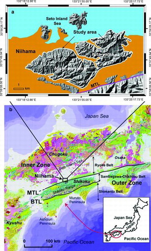
The geology of the Shikoku region is characterized by three distinct units, namely the Ryoke, Sambagawa-Chichibu, and Shimanto Belts. Two northerly dipping major faults, the Median Tectonic Line (MTL) in the north and the Butsuzo Tectonic Line (BTL) in the south, separate the three geological units (Hashimoto 1991; Dahal et al. 2011). The selected study area falls in the Ryoke Belt, and consists of tertiary shales and sandstones of the late Cretaceous age often known as the Izumi group. Typical feature of this geological formation is that piles of intercalated sandstone and shale run in an east–west direction.

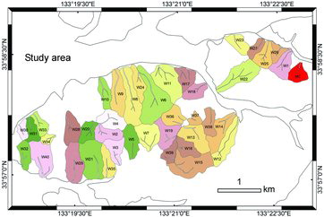
Japan often experiences heavy rainfalls during periods of extreme climate such as a typhoon. June to October is usually the typhoon season in Japan. In 2004, a series of nine typhoons hit Shikoku Island causing extreme typhoon rainfalls of various intensities, which resulted in a massive loss of life and property. Typhoon 0423 and 0421 severely impacted Ehime, Kochi, and Kagawa Prefectures in the region. Niihama city (about 140,000 residents) in Ehime Prefecture was the hardest hit area where many debris flows near the hill bases caused 25 deaths and 40 billion yen worth of property damage (Bhandary and Yatabe 2005). A total of 424 slope failures in September and 1396 slope failures in October were identified to have occurred in the selected area (figure 2). A higher number of slope failures was found in the Kita-yama area than the Nishi-no-yama area. It was later understood that the maximum hourly rainfall exceeded 50 mm and the maximum one-day rainfall exceeded 300 mm, and were the main causes of slope failures (Dahal et al. 2006; Bhandary et al. 2013). Altogether 41 catchments were delineated in the topographical map (figure 2) in the study area. The catchments were selected on the basis of an abundance of both September and October slope failures. Figure 3 shows the selected catchments in detail (indicated by MC and W1-W40; here, MC is the model catchment and others are the test catchments). In this study, both September and October slope failures were utilized separately to assess the prediction accuracy of slope failure hazard maps in the selected test catchments.

Figure 2. Distribution of slope failures of September and October of 2004 in selected catchments of Niihama.

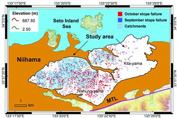
Figure 3. The selected model catchment and test catchments in detail.

3. Methodology

The research framework of this study is illustrated in figure 4. The Higashifukubegawa catchment, indicated by MC in figure 3, was used for the deterministic slope failure hazard assessment. For this, basic geo-mechanical and hydrological properties of soil obtained from various sources were utilized. Both hydrological and stability models were considered in the hazard assessment. Hydrological modelling was done at a hillslope scale. The catchment scale hydrology was derived from the sub-surface hydrology of individual hillslope profiles. The results obtained from the hydrological modelling were then used in stability modelling in pixel basis for the entire model catchment so as to obtain a deterministic slope failure hazard model. The deterministic model thus obtained was then replicated to the test catchments through statistical regression modelling using DEM-derived parameters. The following subsections describe the details of the methods and materials used in the analysis.

Figure 4. Research flow in this study.

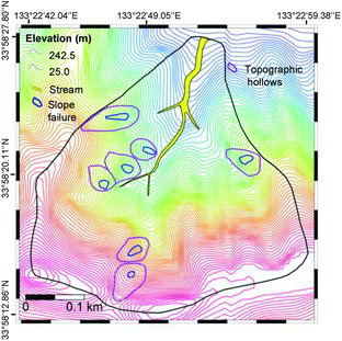
3.1. Model catchment

The Higashifukubegawa catchment has a tentative oval shape (figure 5). It has a spatial extension of 142,000 sq. m and the elevation varies from 2.5 m to 285 m from the mean sea level. The catchment is characterized by steep slopes with shallow colluvium. The slope varies between 0 and 60.57° with a mean value of 32.37°. Almost 2/3 of the catchment has slope between 20° and 40°. A detailed slope failure inventory of the catchment was prepared through field checks, Google Earth Image interpretation and inventories of September and October slope failures of 2004. After this, there were no inventories of September and October slope failures for model catchment. The detailed slope failure inventory contains seven slope failures (figure 5), each lying on separate topographic hollows or zero order basins.

Figure 5. Higashifukubegawa catchment with detailed slope failure inventory, showing slope failures lying in topographic hollows.

3.2. Geo-mechanical and hydrological data collection

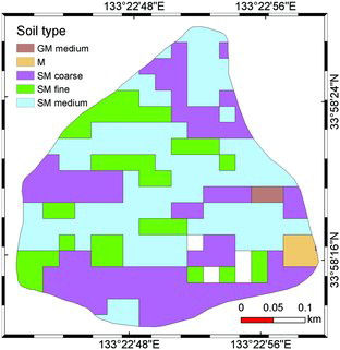
Field visits were made in October, November, December, and April of 2011 as well as November of 2012 in the model catchment to observe the response of catchment slopes during various rainfall events in these months. To obtain detailed in-situ/laboratory data, the model catchment was divided into 25 sq. m blocks. The total number of blocks was 261 (figure 6). The in-situ tests, such as the dynamic cone penetration test to measure the soil thickness above weathered bedrock and the Hasegawa in-situ permeability test (Daitou Techno Green 2009) to measure soil permeability within the unsaturated zone, were conducted in each square block. These tests revealed that soil thickness varied from 0.1 m to 1.91 m and soil permeability from 10⁻⁵ m/s to 10⁻⁸ m/s in the model catchment. At least one soil sampling was done at each block to determine the basic geo-mechanical properties of soil and to classify the soil type. Mohr-Coulomb parameters of soil strength (C′, φ′) were determined from direct shear test results. Root cohesion () was estimated from the findings of Neupane (2005) and information provided by Sidle (1991) for similar types of plants in this study. Also, the laboratory tests for saturated unit weight (γ_sat), bulk unit weight (γ_t), porosity or volumetric water content (n), and particle size distribution of soil were conducted following the specifications of ASTM. Based on the results of particle size distribution (after referring to USCS and ASTM standards), the soils were classified into five major soil domains, namely SM (fine), SM (coarse), SM (medium), GM, and M [SM is silty sand, GM is silty gravel, and M is silt]. The extreme values of geo-mechanical and hydrological properties in five major soil domains are given in table 1. Based on soil domains, the model area was partitioned into five zones (figure 7) for deterministic slope failure hazard modelling (see in Section 3.5).

Table 1. Geo-mechanical and hydrological properties of soil domains

	Major soil domains
	SM (fine)		SM (medium)		SM (coarse)		GM (medium)		M
Soil properties	MIN	MAX	MIN	MAX	MIN	MAX	MIN	MAX	MIN	MAX
C′ (kN/m^2)	0.31	10.76	1.62	14.11	0.31	12.50	4.49	10.85	9.48	12.50
φ′ (°)	23.91	43.59	20.92	40.59	22.15	44.59	21.91	33.14	24.33	34.64
C′r (kN/m^2)	1.92	4.79	0.00	4.79	1.50	4.48	1.92	4.31	1.40	3.35
γt (kN/m^3)	10.58	15.04	11.74	16.74	9.58	14.07	14.44	15.07	11.59	13.94
γsat (kN/m^3)	15.43	18.90	16.33	19.90	15.33	17.39	16.79	17.19	17.43	18.29
n	0.48	0.51	0.45	0.55	0.45	0.52	0.42	0.47	0.41	0.51
k (m/s)	6.12×10^−8	2.66 × 10^−5	7.18 × 10^−8	4.67 × 10^−5	8.01 × 10^−8	3.69 × 10^−5	7.78 × 10^−8	1.48 × 10^−5	6.16 × 10^−8	2.17 × 10^−5

Note: Saturation depth (h) and soil depth (z) data are not included in this table. The spatial distribution of these two properties will be prepared in raster format for the whole model area (see in Section 3.5).

Figure 6. 25 sq. m blocks in model catchment. The hollow blocks representing bedrock were excluded from the analysis.

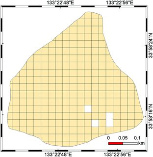
Figure 7. Major soil domains in the model catchment after soil classification.

3.3. Model selection

The reliability of a hazard map depends not only on quality/amount of the incorporated data and working scale but also on appropriate methodology (Baeza and Corominas 2001). The models should be chosen also with climatic realization. For this study, we chose SEEP/W (GeoStudio 2005) as a hydrological modelling tool and considered infinite slopes for the stability modelling. Likewise, we used a discriminant function model (multivariate regression model) for the replication purpose. These models have been acknowledged worldwide in recent landslide research such as Gasmo et al. 2000; Acharya et al. 2006; Godt et al. 2008; Lee et al. 2008; Trandafir et al. 2008; Eeckhaut et al. 2009; Cascini et al. 2010; Tarolli et al. 2011; Ghosh et al. 2012; Harris et al. 2012; and Jagielko et al. 2012. The SEEP/W (GeoStudio 2005) hydrological model is first used in slope failure hazard assessment in this study. The following subsections briefly describe the models.

3.3.1. Hydrological model

As also stated earlier, rainfall is a temporal stochastic phenomenon. The amount of rainfall varies with time (Ng and Shi 1998), and with time varying infiltration, the porewater pressure rises/falls above impervious bedrock. This rise/fall (transient behaviour) of porewater pressure often controls hillslope instability (Reid and Iverson 1992), but it is difficult to estimate the transient porewater pressure information required for the slope stability analysis of hillslopes (Harp et al. 2009). SEEP/W (GeoStudio 2005) solves this problem. It is a finite element mesh model of non-linearized Richard's equation. Richard's equation explains both saturated and unsaturated Darcian flows through soil layers. Richards's equation to compute 2-dimensional seepage in SEEP/W has the following form: (1) where k_x is the coefficient of permeability in the x direction; k_y is the coefficient of permeability in y direction; H is the hydraulic head or total head; q is applied flux at the boundary; m²_w is the slope of soil–water characteristics curve; and γ_w is the unit weight of water. With these inputs, this study uses SEEP/W to compute transient porewater pressure distribution in hillslopes. The computed seepage is then used in the infinite slope stability model.

3.3.2. Infinite slope stability model

The hillslopes with loose soil colluviums can be recognized as infinite slopes when the soil thickness is limited compared to slope length and width, slope gradient is constant throughout the length, and underlying ground water flow is parallel to the ground surface (Taylor 1948). In such slopes, the failure mass is analyzed as the movement of a single block of soil, disregarding the head and toe portions (Arnone et al. 2011). Infinite slopes are easily destabilized due to a rapid rise in positive porewater pressure or a loss of soil suction during rainfall (Iverson et al. 1997). The slope mass fails typically at or near the contact between the soil colluvium and impervious bedrock. Generally, the nature of failure is translational. The shear strength acting along the slip surface is given by the Mohr–Coulomb criterion (Terzaghi and peck 1967). (2) where τ is the shear strength of unsaturated soil; C′ is the effective cohesion (kN/m²); (σ_n − u_w) is the net normal stress; σ_n is the total normal stress (kN/m²); u_w is porewater pressure (kN/m²); and φ′ is the angle of shearing resistance (°). During failure, shear stress (T) exceeds shear strength (τ). The ratio F = τ/T is called the factor of safety. For an infinite slope, the factor of safety can be expressed as below (Hammond et al. 1992). (3)

In which

where is the effective root strength; β is the slope inclination (°); γ_sat (kN/m³) is the saturated unit weight of soil; γ_t (kN/m³) is the bulk unit weight of soil; h is the vertical saturation depth (m); and D is the vertical soil depth (m) (as expressed in Section 3.3.1; h is estimated from hydrological modelling). The effect of surcharge is disregarded in this study. When the factor of safety is greater than 1, the hillslope is stable and when it is equal to 1, the slope mass is on the verge of failure (limit equilibrium state). An infinitesimal perturbation can result in sliding.

The Mohr–coulomb strength parameters (i.e. C′, φ′) computed in the laboratory and the root strength () estimated from past studies may vary from the actual field values. So, these have some degree of uncertainty. The erroneous strength parameters either should not be used (van Westen and Terlien 1996) or the factor of safety computed by using such parameters should be checked for error. Various methods exist in the literature for analyzing the propagation of error (Ward et al. 1981; Hammond et al. 1992; Terlien 1996; Burrough and McDonnell 1998). Calculating the expected value and the variance of the factor of safety and incorporating these into a stability analysis to compute a z-score is a reliable method (Dahal et al. 2008b). Based on these, equation 4 is converted in the following linear form. (4) where

In this study, the expected value and variance of the factor of safety, and the z-score are ascertained by using the following equations (Ward et al. 1981; Ross 2004). (5) (6) (7) where, E[.] is the expected value; V[.] is the variance, and Z is the z-score. The expected values and variance of the Mohr–Coulomb strength parameters are computed based on their nature of distribution (see in Section 3.5). E[FS] is the average value of the factor of safety. V[FS] gives the total propagation of error due to the variation of C′, _, and tanφ′. The z-score is equivalent to the corrected factor of the safety score or the factor of safety score after adjusting for error. It is considered as the susceptibility/hazard score (Guzzetti et al. 2005; Dahal et al. 2008b). In this study, the failure probability score is computed from the z-score that is then implemented into ILWIS 3.8.1 to prepare the slope failure probability map. Thus, with the availability of geo-mechanical (C′, C′_r, φ′, γ_sat, γ_t), hydrological (h), and geometric properties (β), the evaluation of hillslope instability or slope failure hazard is possible as carried out in this study.

3.3.3. Discriminant function model

The discriminant function model is used to determine the relationship between the outcome or the dependent variable (e.g. slope failure) and the independent or predictor variables (causal factors of slope failure) (Nagarajan et al. 2000; Carrara et al. 2003; Ghosh et al. 2012; Jagielko et al. 2012). This model is required when there are multiple (i.e. >2) categories of dependent variables (e.g. types of failures). The model determines multiple combinations of employed independent variables (which are the discriminant functions) and selects the most significant combination (it is the combination that best discriminates categories of dependent variables) (Baeza et al. 2010; Dong et al. 2009). For example, if there are m categories of dependent variables, the possible combination of independent variables or discriminant functions will be m-1. Finally, the selected combination of variables is included in the discriminant function equation. The discriminant function equation is a linear combination of weighted independent variables as given below. (8)

Where DFs is the discriminant function score; b_o is the coefficient that maximizes the variability between categories of dependent variables; b_n is the discriminant weight value or discriminant coefficient. The negative/positive sign of the discriminant weight values determine the contribution of employed independent variables to discriminant categories of dependent variables (or these determine the significance of independent variables to cause instability); X_n is the most significant combination of independent variable (slope failure causal factor). The goodness of fit of the discriminant function model was tested using the Wilk's lambda test (Baeza et al. 2010; Jamaludin et al. 2006; Ghosh et al. 2012; He et al. 2012). The Wilk's Lambda score measures the discriminating potential of a combination of parameters. The smaller the value of Wilk's Lambda, the higher the discriminating capability. Hence, a small value of Wilk's Lambda (<1) is always preferred in discriminant function analysis. In the Wilk's Lambda test, if the significance of the Chi-square value is less than 0.05, the combination of parameters is significant and the discriminant function model can be accepted (Baeza et al. 2010, Ghosh et al. 2012). In this study, different low and high hazard classes of the deterministic slope failure hazard model were used as categories of dependent variables and slope failure causal factors (DEM-based parameters) as independent variables in discriminant function modelling.

3.4. Seepage modelling

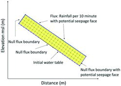
Seepage modelling was performed in SEEP/W (GeoStudio 2005) to obtain porewater pressure information required for the slope stability analysis in the model catchment. For this, 55 slope profiles were drawn in the model area parallel to the direction of maximum subsurface flow. Their locations are represented by slope profile lines in figure 8. The profile geometry of these lines was prepared using DEM (5 m resolution) of the study area and the soil thickness data considering the topographical break in slope (figure 9). All the profile continuums were discretized into a mesh of fine squares of four nodes and a nine-integration order. The dimensions of all the elements were the same with a side length of <0.2 m and unit thickness. The soil water characteristics curve (SWCC) and soil permeability were the two major input parameters required for the seepage simulation of each profile unit. For this, the mean values of volumetric water content (porosity) and soil permeability of all the square blocks lying below slope profile were computed for each slope profile. The computed mean values were integrated with SWCC and the soil permeability functions available in the SEEP/W library. SEEP/W is highly sensitive to initial ground water table conditions. To prevent an unnecessary negative porewater pressure regime, a limiting value of −20 kPa suction was applied as the initial condition. The initial ground water table was defined along the boundary between the soil colluvium and the bedrock. Boundary conditions control porewater pressure distribution along the profile length. A null flux boundary condition was applied on the left vertical edge, the right vertical edge, and along the bedrock (figure 10). The phreatic line itself acts as the upper boundary along the exposed sloping face. The potential seepage face was considered to be on the right vertical edge and along the exposed sloping face to avoid ponding on the slope.

Figure 8. Slope profile lines constructed in the entire model catchment.

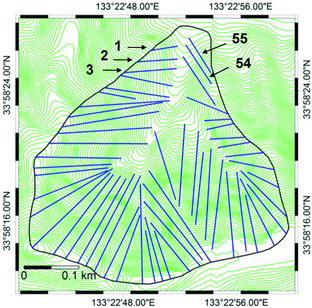
Figure 9. Typical examples of geometrical configurations of slope profiles 1, 2, 3, 4, 5, and 6 (from figure 7).

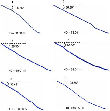
Figure 10. Boundary conditions applied to finite element mesh model.

There was considerable rainfall almost every day in October 2004 and slope failure occurred on October 20, but no data were available for porewater pressure variation that could describe the initial seepage condition in the slopes prior to the rainfall events. So, the initial seepage conditions were disregarded and the simulation was preceded with the precipitation data of October 19–20. Two days of hourly rainfall data were discretized into 283 time steps of 10 min in length and applied onto the exposed face of the profiles from upward at an equal pressure head and elevation condition. Transient pore water pressure lines (transient pore water pressure distributions) were developed at each time step. The ground water tables at succeeding time steps had higher depths compared to the preceding ones along each profile length due to the accumulation of rainfall above the bedrock. The peak hourly rainfall intensity was at 12:00 noon on 20 October 2004. There was no eyewitness for the exact time of failure on 20 October, but the peak porewater pressure reached two hours after peak rainfall hour (i.e. at 14:00 rainfall hour) on the same day in all simulations. This implies that the slope failure in the model catchment might have begun at 14:00 hours of rainfall on 20 October (i.e. the 38 hours of continuous rainfall on 19–20 October). Owing to this, the ground water table, which developed at 14:00 hours of rainfall on 20 October 2004, was decided to implement in limit equilibrium analysis. The vertical depth of saturation was recorded at various points along each slope profile in the selected ground water table. With these data, a point map of saturation depths was prepared.

3.5. Deterministic slope failure hazard modelling

The geo-mechanical and hydrological properties (table 1) of hillslope materials were parameterized in the ILWIS 3.8.1 platform. The point map of soil depth (prepared in field) and saturation depth (prepared from seepage modelling) covering the entire model area were digitized. The spatial correlation of both data was investigated. The spatial correlation provides a semivariogram model about the spatial behaviour of the soil properties (Jorge 2009). The rotational Quadratic semivariogram model was best fitted by both digital soil depth and saturation depth data [figure 11 (a, b, c)], and this model yielded values of nugget, sill, and range for each data type. These three parameters were inputs to the Kriging interpolation along with the respective soil spatial properties. With the ordinary Kriging interpolation method, the randomly distributed point values of soil depth and saturation depth are converted into regularly distributed grid values. To prepare the saturated unit weight and the bulk unit weight map, first the average value of these properties (table 1) were computed for each zone of the model area and then converted into a raster image using ILWIS functions. To prepare the expected and variance maps of the strength parameters (C′, , φ′), the uniform distribution of these properties was assumed in the entire model area. For uniformly distributed data, the expected values and variance are computed using the following relationships: (9) (10)

Figure 11. Rotational quadratic semi-variogram models to estimate spatial distribution of (a) soil depth and (b) saturation depth in model catchment. Nugget, sill, and range were fit parameters for both models, which is illustrated in (c).

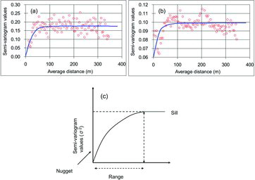
Figure 12. Slope failure probability map.

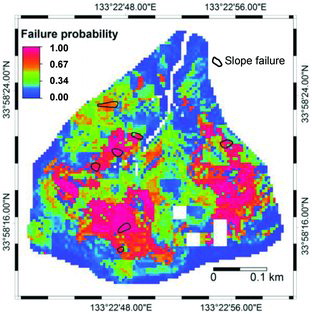
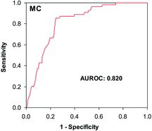
Figure 13. Area under ROC curve estimated from Higashifukubegawa catchment after deterministic slope failure hazard modelling.

where where a and are minimum and maximum values of strength parameters. These values were employed to compute the expected values and variances of the strength parameters for each zone outside ILWIS. The computed expected values and variances were then imported into ILWIS and converted into a generalized continuous raster form. The slope gradient map was obtained from the DEM of the model catchment. All these maps were used for deterministic slope failure hazard modelling.

To obtain a robust deterministic slope failure hazard model, a complete parametric analysis was performed by varying shear strength parameters (C′, , φ′). The expected map and variance map of factor of safety were prepared on a cell-by-cell basis (5 m resolution) using equations 5 and 6. These maps were directly implemented in the z-score computation (equation 7). The z-score herein is the slope failure hazard score. The area under the standardized normal weights of the z-score between F = 1 and Z = −∞ gives failure probability. In the case with large voluminous data, as in the present study, the commercially available spreadsheet software can be utilized to calculate probability from the z-score (Dahal et al. 2008b). In this study, the z-score was exported to Microsoft Excel and the NORMSDIST function was employed to compute probability. This process of calculation of failure probability is in accordance with Terlien (1996) and van Westen and Terlien (1996). The probability value computed in excel was imported into ILWIS and rasterized to prepare the slope failure probability map. This map was validated using the detailed slope failure inventory of the model catchment. The hazard classes were determined by visual inspection of the distribution of pixels with higher values of probability from the ROC prediction rate. Generally, high-hazard classes consist of pixels with high probability values (the greatest number of pixels where slope failures occurred) and low hazard classes cover the regions of low probability values (the fewest number of slope failure pixels). Finally, the zonation map was once again crosschecked with the detailed slope failure inventory for spatial agreement.

3.6. Replication of deterministic model and accuracy check

After confirming a good predictive success rate from the validation, the results of the deterministic slope failure hazard model were applied to 40 selected test catchments of the study area. For this, first discriminant function modelling was carried out amongst the deterministic model and causal factors of slope failure, and the discriminant function equation was obtained for the model catchment. Using this equation and using the same set of seven DEM-based slope failure causal parameters, the slope failure hazard index maps were obtained in the test catchments. These maps were compared separately with the prevailing slope failure inventories of September and October 2004 to check their prediction accuracy.

4. Results

4.1. Deterministic modelling

Figure 12 shows the slope failure probability map obtained after performing full parametric modelling of shear strength parameters. To validate this map against the detailed slope failure inventory, the ROC curve (AUROC) method (Zweig and Campbell 1993) was used. It determines the predictive capability of a model (Yesilnacar and Topal 2005; Van Den Eeckhaut et al. 2006). The ROC makes a diagnosis for spatial agreement of prevailing slope failures with the failure probability score. The variables used in ROC curve analysis in SPSS are a binary (0-1) map of the slope failure inventory and the failure probability score. Based on the degree of spatial matching between these two variables, the ROC curve method determines the area under the ROC curve (AUROC). This area is the measure of the robustness of the model to predict future slope failures. The AUROC value of the model catchment based on its detailed slope failure inventory was 0.82 (figure 13). The ROC curve also suggests that about 68% of the slope failure numbers were concentrated in areas showing upper 20% of the failure probability index. These reasonably verify the ability of the model to predict future slope failures.

Figure 14. Slope failure hazard zonation map of Higashifukubegawa catchment (deterministic model).

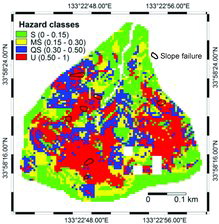
Figure 15. Slope failure distribution in hazard classes of zonation map.

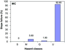
Based on the ROC prediction rate and the coverage of a higher percentage of slope failure at a higher value of probability, the slope failure probability map was classified into four hazard classes: Stable (S, <30% probability value), Metastable (MS, 30%–50% probability value), Quasi-stable (QS, 50%–70% probability value), and Unstable (U, 70%–100% probability value) (figure 14), which is from a low- to a high-hazard level. The classes were assigned the colours green, yellow, blue, and red, respectively. This is the deterministic slope failure hazard model in the Higashifukubegawa catchment. Finally, the zonation map was crossed with the raster map of the detailed slope failure inventory. The result (figure 15) shows that a total of 92.6% of the slope failures were found to occur in the U class, which is very promising. Also, only a few pixels of slope failures were located in the QS and MS classes (which are 1.90% and 5.60% of the total slope failures, respectively). There was no slope failure pixel in S class.

Figure 16. Slope failure hazard index maps of catchments W20 and W30 after application of discriminant function weight values of each parameters from Higashifukubegawa catchment (HI: Hazard Index).

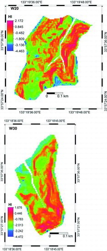
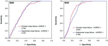
Figure 17. Area under ROC curve estimated from slope failure hazard index score of catchments W20 and W30 after replication of deterministic model.

4.2. Discriminant function modelling

As mentioned earlier, the categories of dependent variables and independent variables are required to obtain a discriminant function equation. Here, the four hazard classes of the deterministic model: S, MS, QS, and U were used as categories of dependent variables. A failure probability number: 1, 2, 3, and 4 was assigned to the classes from a low- to a high-hazard class. Similarly, a set of seven significant and easily available topographical and hydro-geological parameters, namely slope, relief, plan curvature, profile curvature, wetness index, flow accumulation, and drainage density, were selected as the independent variables in model catchment. All of these parameters were derived from DEM (5 m resolution). With inputs of the above-mentioned dependent and independent variables, the discriminant function modelling was performed in the SPSS platform. The results of the discriminant function modelling are presented in tables 2–4

Table 2. Unstandardized canonical discriminant function coefficients.

	Functions
Parameters	1	2	3
Slope	0.101	0.003	0.012
Relief	−0.0000178	0.017	0.009
Plan curvature	−0.014	−0.047	0.362
Profile curvature	−0.755	0.321	0.328
Wetness index	0.067	−0.118	0.314
Flow accumulation	−0.0003190	−0.001	0.0000708
Draining density	7.565	−8.124	36.413
Constant	−3.711	−1.454	−3.651

Table 3. Wilk's lambda test.

Function (s)	Wilk's lambda	Chi-square	df	Sig.
1 through	0.705	1932.105	21	0.000
2 through	0.987	74.947	12	3.76E-11
3	0.996	23.394	5	2.84E-04

Table 4. Standardized canonical discriminant function coefficients.

	Functions
Parameters	1	2	3
Slope	0.988	0.027	0.114
Relief	−0.00100	0.874	0.459
Plan curvature	−0.016	−0.052	0.400
Profile curvature	−0.207	0.088	0.090
Wetness index	0.112	−0.198	0.524
Flow accumulation	−0.10500	0.229	0.023
Draining density	0.174	−0.187	0.837

Table 5. ROC prediction rates for test catchments.

	Prediction rate
Catchment ID	October slope failure	September slope failure
W1	0.704	0.743
W2	0.732	0.726
W3	0.731	0.752
W4	0.727	0.740
W5	0.762	0.789
W6	0.751	0.734
W7	0.754	0.736
W8	0.794	0.759
W9	0.790	0.814
W10	0.760	0.814
W11	0.788	0.741
W12	0.761	0.768
W13	0.755	0.719
W14	0.788	0.760
W15	0.773	0.783
W16	0.772	0.788
W17	0.791	0.772
W18	0.741	0.753
W19	0.776	0.780
W20	0.750	0.757
W21	0.805	0.802
W22	0.798	0.784
W23	0.733	0.746
W24	0.763	0.807
W25	0.743	0.730
W26	0.763	0.784
W27	0.734	0.743
W28	0.741	0.789
W29	0.790	0.752
W30	0.803	0.794
W31	0.800	0.796
W32	0.783	0.799
W33	0.727	0.765
W34	0.738	0.773
W35	0.744	0.763
W36	0.735	0.721
W37	0.743	0.735
W38	0.725	0.747
W39	0.783	0.735
W40	0.805	0.770

The discriminant function model produced three combinations of casual parameters of slope failure or discriminant functions (table 2), which was 1 less than the number of the hazard classes of the deterministic model. All three combinations of the parameters were found significant since the significance of the Chi-square value was less than 0.05 in all combinations (table 3). However, the lowest Wilk's Lambda score (0.734) and significance level (0.00) of the first combination enable us to confirm that the first combination is the most significant among the three (i.e. it most discriminates the hazard classes of the deterministic model or the group means are significantly different for this combination). Based on these results, the first combination of parameters or the discriminant function is included in the discriminant function equation. The discriminating potential of the employed independent slope failure causal parameters to the hazard classes can be understood from the Standardized Canonical Discriminant Function Coefficients listed in table 4

4.3. Replication and validation

To apply the results from discriminant function modelling, the same set of seven DEM-derived slope failure causal parameter maps were prepared in all the test catchments. The discriminant weight values of the parameters of the model catchment were applied to the corresponding parameters of the test catchments and the discriminant function equation was portrayed to compute the discriminant function score or the slope failure hazard index. Figure 16 shows the resulting slope failure hazard index maps of two typical test catchments W20 and W30. The slope failure hazard score was more or less similar in all 40 catchments. To check the prediction accuracy, the resulting hazard maps were crossed with the existing inventories of the September and October slope failures of 2004, and the ROC curves were plotted. The area under the ROC curve gives the prediction rate. Figure 17 exhibits the prediction rate obtained with hazard index maps of catchments W20 and W30. The prediction rate with respect to the September and October slope failures in 40 test catchments is summarized in table 5. From this table, it is understood that the prediction rate was higher with the inventory of the September slope failure in 22 test catchments (W1, W3, W4, W5, W9, W10, W12, W16, W17, W18, W19, W20, W21, W22, W25, W26, W28, W29, W32, W36, W37, and W38) whereas in the remaining test catchments, the prediction rate was higher with the inventory of the October slope failure. Overall, the prediction rates from 0.719 to 0.814 and 0.704 to 0.805 were noted with the inventories of September and October slope failures, respectively, from table 5. This implies that the prediction of the September slope failure was better than the October slope failure by approximately 1%. However, a moderate-to-good prediction accuracy was obtained with both inventories for spatial agreement.

5. Discussion

In this study, deterministic slope failure hazard analysis was carried out in the Higashifukubegawa catchment. But, this kind of analysis can not be conducted in any of the other test catchments since it is very difficult to obtain the detailed geo-mechanical and hydrological properties of soils required for the analysis. Therefore, it is necessary to explore for replication methodology that incorporates the deterministic model and can predict the slope failure hazard in catchments of similar geological and geomorphological settings. In this study, we have presented and examined the replication process of a deterministic slope failure hazard model in numerous catchments of the selected study area. The deterministic model prepared for the Higashifukubegawa catchment included an area under ROC as 0.82, which is a good success rate. The results of the deterministic model from Higashifukubegawa were then replicated through discriminant function modelling using DEM-based parameters. In this research, it is assumed that the underlying physical processes associated with hillslope failures would be the same in similar geological/geomorphological settings and if the index properties of the soil do not vary significantly. Under such conditions, hillslopes fail in a similar way or under the same combination of parameters.

The discriminant function modelling performed between the deterministic model and a set of seven DEM-based parameters (i.e. slope, relief, plan curvature, profile curvature, wetness index, flow accumulation, and drainage density) in the model catchment resulted in a significant combination of parameters or discriminant function with Wilk's lambda (0.705), the Chi-square value (1932.105), and the significance level of the Chi-square value (0.000). As a result, the model characteristics were transferred into an empirical parametric relationship known as a discriminant function equation. This relationship was applied to 40 test catchments of the study area with the same set of DEM-based parameters and slope failure hazard index maps were obtained. In the results, the prediction accuracies were found to vary over a wide range, from moderate to good with both inventories. In a few catchments, the accuracy was in the same range of model accuracy rate (0.82). From this, it is well understood that if replication of a deterministic model is carried out employing parameters-based multivariate regression modelling, the prediction accuracy can be significantly increased. Replication of slope failure hazard, as in the present study, can be reviewed in a very few catchment-scale studies, such as Ghimire 2011 and Dahal et al. 2012 with a similar reasonable performance. However, this study has first indicated the possibility of the replication of a deterministic slope failure hazard model, although research on the deterministic shallow landslide hazard assessment or physically based modelling of shallow landslides has been practised worldwide for the past few decades (Montgomery and Dietrich 1994; Borga et al. 1998; Moon and Blackstock 2004; Rosso et al. 2006; Meisina and Scarabelli 2007; Dahal et al. 2008b; Godt et al. 2008; Salciarini et al. 2008; Sorbino et al. 2010). The parametric relation obtained in the Higashifukubegawa catchment can be used to predict slope failure hazard conditions in other areas with similar geological/geomorphological characteristics if the DEM-based parameters are available. Further, the replication of a deterministic model could be performed with higher accuracy if enough considerations were given to the quality of the geo-mechanical and hydrological parameters in model catchments as well as the quality of the DEM-based parameters.

6. Conclusions

From this work, we conclude with the following statements.

1. We were successful in connecting hillslope-scale (local-scale) sub-surface hydrology to catchment-scale (landscape-scale) sub-surface hydrology.

2. We understood that the geo-mechanical and hydrological properties of hillslope materials are the key controlling factors of slope failure hazard in tertiary sedimentary terrain in the Shikoku Region of Japan.

3. We have obtained 0.719–0.814 and 0.704–0.805 prediction accuracy rates for the spatial prediction of slope failures of the 2004 September and October slope failure inventories, respectively. This reasonably validates the model and replication process.

4. We have been successful in replicating the model through parameters-based multivariate modelling for the purpose of predicting the slope failure hazard index without using geo-mechanical and hydrological parameters.

5. Finally, the work in this study indicates that the replication process used here to predict the slope failure hazard condition on a small-catchment scale has a wide applicability in other areas of similar geological and geomorphological characteristics.

Acknowledgements

We are thankful to Mr Masatoshi Anakura and Dr Manita Timilsina (former graduate students of Ehime University) for their help in field/laboratory data preparation.

References

- Acharya G, Smedt F De, Long NT. 2006. Assessing landslide hazard in GIS: a case study from Rasuwa, Nepal. Bull Eng Geology Environ. 65:99–107.
- Aleotti P, Chowdhury R. 1999. Landslide hazard assessment: summary review and new perspectives. Bull Eng Geology Environ. 58:21–44.
- Arnone E, Noto LV, Lepore C, Bras RL. 2011. Physically-based and distributed approach to analyze rainfall-triggered landslides at watershed scale. Geomorphology. 133:121–131.
- Baeza C, Corominas J. 2001. Assessment of shallow landslide susceptibility by means of multivariate statistical techniques. Earth Surface Processes Landforms. 26:1251–1263.
- Baeza C, Lantada N, Moya J. 2010. Validation and evaluation of two multivariate statistical models for predictive shallow landslide susceptibility mapping of the Eastern Pyrenees (Spain). Environ Earth Sci. 61:507–523.
- Barredo J, Benavides A, Hervas J, van Westen CJ. 2000. Comparing heuristic landslide hazard assessment techniques using GIS in the Tirajana basin, Gran Canaria Island, Spain. Int J Appl Earth Observation Geoinformation. 2:9–23.
- Bell R. 2007. Lokale und regionale gefahren- und risikoanalyse gravitativer massenbewegungen an der schwäbischen Alb [Local and regional hazard and risk analysis of gravitational mass movements at the Swabian Jura]. Bonn (Germany): University of Bonn German.
- Bhandary NP, Dahal RK, Timilsina M, Yatabe R. 2013. Rainfall event-based landslide susceptibility zonation mapping. Nat Hazards. 69:365–388.
- Bhandary NP, Yatabe R. 2005. Influence of precipitation pattern on triggering surface-layer failures of slopes during 2004 Niihama disasters. In: Proceedings of the One-day Symposium on Geo-disasters and Geo-environment, Ehime (Japan): Ehime University; p. 63–70.
- Bijukchhen SM, Kayastha P, Dhital MR. 2013. A comparative evaluation of heuristic and bivariate statistical modelling for landslide susceptibility mappings in Ghurmi–Dhad Khola, East Nepal. Arab J Geosciences. 6(8):2727–2743.
- Borga M, Fontana GD, Ros DD, Marchi L. 1998. Shallow landslide hazard assessment using a physically based model and digital elevation data. J Environ Geol. 35:81–88.
- Burrough PA, McDonnell RA. 1998. Principles of geographical information systems. Oxford: Oxford University Press.
- Cannon SH, Gartner JE, Rupert MG, Michael JA. 2004. Emergency assessment of debris-flow hazards from basins burned by the Padua fire of 2003, southern, California (US Geological Survey Open-File Report 2004–1072). Reston (VA): US Geological Survey; p. 14.
- Carrara A, Crosta GB, Frattini P. 2003. Geomorphological and historical data in assessing landslide hazard. Earth Surf Process Landf. 28:1125–1142.
- Carrara A, Guzzetti F, Cardinali M, Reichenbach P. 1999. Use of GIS technology in the prediction and monitoring of landslide hazard. Nat Hazards. 20:117–135.
- Cascini L, Cuomo S, Pastor M, Sorbino G. 2010. Modeling of rainfall-induced shallow landslides of the flow-type. J Geotech Geoenviron Eng. 136(1):85–98.
- Ching J, Liao HJ, Lee JY. 2011. Predicting rainfall-induced landslide potential along a mountain road in Taiwan. Geotechnique. 61:153–166.
- Crosta G. 1998. Regionalization of rainfall thresholds: an aid to landslide hazard evaluation. Environ Geol. 35:131–145.
- Crozier MJ. 1999. Prediction of rainfall-triggered landslides: a test of the Antecedent Water Status Model. Earth Surf Process Landf. 24(9):825–833.
- Dahal RK, Hasegawa S, Bhandary NP, Poudel PP, Nonomura A, Yatabe R. 2012. A replication of landslide hazard mapping at catchment scale. Geomatics, Nat Hazards Risk. 3: 161–192.
- Dahal RK, Hasegawa S, Nonomura A, Yamanaka M, Dhakal S. 2008b. DEM-based deterministic landslide hazard analysis in the Lesser Himalaya of Nepal. Georisk: Assess Manag Risk Eng Syst Geohazards. 2:161–178.
- Dahal RK, Hasegawa S, Nonomura A, Yamanaka Y, Dhakal S, Paudyal P. 2008a. Predictive modelling of rainfall-induced landslide hazard in the Lesser Himalaya of Nepal based on weights-of-evidence. Geomorphology. 102:496–510.
- Dahal RK, Hasegawa S, Yamanaka M, Bhandary NP, Yatabe R. 2011. Rainfall-induced landslides in the residual soil of andesitic terrain, western Japan. J Nepal Geol Soc. 42: 127–142.
- Dahal RK, Hasegawa S, Yamanaka M, Nishino K. 2006. Rainfall triggered flow-like landslides: understanding from southern hills of Kathmandu, Nepal and northern Shikoku, Japan. In: Proceedings of the 10th Int Congr of IAEG ; 2006 Sep 6–10; Nottingham, UK. London: The Geological Society of London. IAEG2006 Paper no. 819, p. 1–14. (CD-ROM).
- Dai FC, Lee CF, Ngai YY. 2002. Landslide risk assessment and management: an overview. Eng Geol. 64(1):65–87.
- Daitou Techno Green. 2009. Hasegawa in situ permeability tester, operating manual. v. 3.1. Available from: http://www.daitoutg.co.jp/prd/pdf/tousui0703.pdf
- D’Odorico P, Fagherazzi S. 2003. A probabilistic model of rainfall-triggered shallow landslides in hollows: a long-term analysis. Water Resour Res. 39:1262. doi:10.1029/2002WR001595.
- Dong JJ, Tung YH, Chen CC, Liao JJ, Pan YW. 2009. Discriminant analysis of the geomorphic characteristics and stability of landslide dams. Geomorphology. 110:162–171.
- Eeckhaut MVD, Reichenbach P, Guzzetti F, Rossi M, Poesen J. 2009. Combined landslide inventory and susceptibility assessment based on different mapping units: an example from the Flemish Ardennes, Belgium. Nat Hazards Earth Syst Sci. 9:507–521.
- Gasmo JM, Rahardjo H, Leong EC. 2000. Infiltration effects on stability of a residual soil slope. Comput Geotechnics. 26:145–165
- GeoStudio. 2005. GeoStudio Tutorials includes student edition lessons. 1st ed. Calgary (Canada): Geo-Slope International.
- Ghimire M. 2011. Landslide occurrence and its relation with terrain factors in the Siwalik Hills, Nepal: case study of susceptibility assessment in three basins. Nat Hazards. 56:299–320.
- Ghosh S, van Westen CJ, Carranza EJM, Jetten VG, Cardinali M, Rossi M, Guzzetti F. 2012. Generating event-based landslide maps in a data-scarce Himalayan environment for estimating temporal and magnitude probabilities. Eng Geol. 128:49–62.
- Godt JW, Baum RL, Savage WZ, Salciarini D, Schulz WH, Harp EL. 2008. Transient deterministic shallow landslide modeling: requirements for susceptibility and hazard assessments in a GIS framework. Eng Geol. 102:214–226.
- Guzzetti F, Reichenbach P, Ardizzone F, Cardinali M, Galli M. (2006). Estimating the quality of landslide susceptibility models. Geomorphology. 81:166–184.
- Guzzetti F, Reichenbach P, Cardinali M, Galli M, Ardizzone F. 2005. Probabilistic landslide hazard assessment at the basin scale. Geomorphology. 72:272–299.
- Hadmoko DS, Lavigne F, Sartohadi J, Hadi P, Winaryo. 2010. Landslide hazard and risk assessment and their application in risk management and landuse planning in eastern flank of Menoreh Mountains, Yogyakarta Province, Indonesia. Nat Hazards. 54:623–642.
- Hammond C, Hall D, Miller S, Swetik P. 1992. Level I Stability Analysis (LISA), documentation for Versito 2.0, Gen. Tech. Rep. INT-285. Ogden (UT): Department of Agriculture, Forest Service, Intermountain Research Station; p. 190.
- Harp EL, Reid ME, McKenna JP, Michael JA. 2009. Mapping of hazard from rainfall-triggered landslides in developing countries: examples from Honduras and Micronesia. Eng Geol. 104(3–4):295–311.
- Harris SJ, Orense RP, Itoh K. 2012. Back analyses of rainfall-induced slope failure in Northland Allochthon formation. Landslides. 9:349–356.
- Hashimoto M, editor. 1991. Geology of Japan. Tokyo: Terra Sci. Pub.; p. 249.
- He S, Pan P, Dai L, Wang H, Liu J. 2012. Application of kernel-based Fisher discriminant analysis to map landslide susceptibility in the Qinggan River delta, Three Gorges, China. Geomorphology. 171–172:30–41.
- Iverson RM, Reid ME, LaHusen RG. 1997. Debris-flow mobilization from landslides. Annu Rev Earth Planetary Sci. 25:85–138.
- Jagielko L, Martin YE, Sjogren DB. 2012. Scaling and multivariate analysis of medium to large landslide events: Haida Gwaii, British Columbia. Nat Hazards. 60:321–344.
- Jamaludin S, Huat BBK, Omar H. 2006. Evaluation of slope assessment systems for predicting landslides of cut slopes in granitic and meta-sediment formations. American J Environ Sci. 2(4):135–141.
- Jia N, Mitani Y, Xie M, Djamaluddin I. 2012. Shallow landslide hazard assessment using a three-dimensional deterministic model in a mountainous area. Comput Geotechnics. 45:1–10.
- Jorge LAB. 2009. Soil erosion fragility assessment using an impact model and geographic information system. Sci Agric. (Piracicaba, Braz.). 66:658–666.
- Lee CT, Huang CC, Lee JF, Pan KL, Kin ML, Dong JJ. 2008. Statistical approach to earthquake induced landslide susceptibility. Eng Geol. 100:43–58.
- Meisina C, Scarabelli S. 2007. A comparative analysis of terrain stability models for predicting shallow landslides in colluvial soils. Geomorphology. 87:207–223.
- Montgomery DR, Dietrich WE. 1994. A physically based model for the topographic control on shallow landsliding. Water Resour Res. 30:1153–1171.
- Moon V, Blackstock H. 2004. A Methodology for assessing landslide hazard using deterministic stability models. Nat Hazards. 32(1):111–134.
- Nagarajan R, Roy A, Vinod Kumar R, Mukherjee A, Khire MV. 2000. Landslide hazard susceptibility mapping based on terrain and climatic factors for tropical monsoon regions. Bull Eng Geol Environ. 58:275–287.
- Neupane RR. 2005. Experimental analysis of strength of local grass and shrub roots used for slope stabilization, Thesis No. 059/MSW/418. Nepal: Master of Science in Water Resources Engineering, Institute of Engineering, Tribhuvan University; p. 85.
- Ng CWW, Shi Q. 1998. A numerical investigation of the stability of unsaturated soil slopes subjected to transient seepage. Comput Geotechnics. 22:1–28.
- Pavel M, Fannin RJ, Nelson JD. 2008. Replication of a terrain stability mapping using an artificial neural network. Geomorphology. 97:356–373.
- Pradhan B, Oh H-J, Buchroithner M. 2010, Weights-of-evidence model applied to landslide susceptibility mapping in a tropical hilly area. Geomatics Nat Hazards Risk. 1:199–223.
- Reid ME, Iverson RM. 1992. Gravity-driven groundwater flow and slope failure potential: 2. Effects of slope morphology, material properties, and hydraulic heterogeneity. Water Resour Res. 28:939–950.
- Ross SM. 2004. Introduction to probability and statistics for engineers and scientists. 3rd ed. Delhi (India): Academic Press (an imprint of Elsevier).
- Rosso R, Rulli MC, Vannucchi G. 2006. A physically based model for the hydrologic control on shallow landsliding. Water Resour Res. 42:W06410. doi: 10.1029/2005WR004369.
- Saha AK, Gupta RP, Arora MK. 2002. GIS-based landslide hazard zonation in the Bhagirathi (Ganga) valley, Himalayas. I J Remote Sens. 23(2):357–369.
- Salciarini D, Godt JW, Savage WZ, Baum RL, Conversini P. 2008. Modeling landslide recurrence in Seattle, Washington, USA. Eng Geol. 102:227–237.
- Segoni S, Rossi G, Catan F. 2012. Improving basin scale shallow landslide modelling using reliable soil thickness maps. Nat Hazards. 61:85–101.
- Sidle RC. 1991. A conceptual model of changes in root cohesion in response to vegetation management. J Environ Qual. 20:43–52.
- Soeters R, van Westen CJ. 1996. Slope instability recognition, analysis, and zonation. In: Turner AK, Schuster RL, editors, Landslides — investigation and mitigation. Transp. Res. Board Special Rep. Vol. 247. Washington DC: National Academy Press; p. 129–177.
- Sorbino G, Sica C, Cascini L. 2010. Susceptibility analysis of shallow landslides source areas using physically based models. Nat Hazards. 53:313–332.
- Talebi A, Uijlenhoet R, Troch PA. 2008. Application of a probabilistic model of rainfall-induced shallow landslides to complex hollows. Nat Hazards Earth Syst Sci. 8:733–744.
- Tarolli P, Borga M, Chang KT, Chiang SH. 2011. Modeling shallow landsliding susceptibility by incorporating heavy rainfall statistical properties. Geomorphology. 133:199–211.
- Taylor DW. 1948. Fundamentals of soil mechanics. New York (NY): Wiley.
- Terlien MTJ. 1996. Modelling spatial and temporal variations in rainfall-triggered landslides. [dissertation]. Enschede (The Netherlands): ITC Publication.
- Terlien MTJ, Van Westen CJ, Van Asch TW. 1995. Deterministic modelling in GIS-based landslide hazard assessment. In: Carrara A, Guzzetti F, editors. Advances in natural and technological hazard research. Dordrecht: Kluwer Academic Publishers; p. 51–77.
- Terzaghi K, Peck RB. 1967. Soil mechanics in engineering practice. Hoboken (NJ): Wiley Intersci.
- Trandafir AC, Sidle RC, Gomi T, Kamai T. 2008. Monitored and simulated variations in matric suction during rainfall in a residual soil slope. Environ Geol. 55:951–961.
- Van Asch Th.WJ, Buma J, Van Beek LPH. 1999. A view on some hydrological triggering systems in landslides. Geomorphology. 30:25–32.
- Van Den Eeckhaut M, Vanwalleghem T, Poesen J, Govers G, Verstraeten G, Vanderkerckhove L. 2006. Prediction of landslide susceptibility using rare events logistic regression: a case-study in Flemish Ardennes (Belgium). Geomorphology. 76:392–410.
- van Westen CJ, Terlien TJ. 1996. An approach towards deterministic landslide hazard analysis in GIS. A case study from Manizales (Colombia). Earth Surf Process Landf. 21:853–868.
- Wang X, Zhang L, Wang S, Lari S. 2013. Regional landslide susceptibility zoning with considering the aggregation of landslide points and the weights of factors. Landslides. doi: 10.1007/s10346-013-0392-6.
- Ward TJ, Li RM, Simons DB. 1981. Use of a mathematical model for estimating potential landslide sites in steep forested basin. In: Davis TRH, Pearce AJ, editors. Erosion and sediment transport in Pacific Rim steep lands. International Hydrological Science Publ No. 132. Wallingford, (Oxfordshire): Institute of Hydrology; p. 21–41.
- Wieczorek GF, Glade T. 2005. Climatic factors influencing occurrence of debris flows. In: Jakob M, Hungr O, editors. Debris-flow hazards and related phenomena. Berlin: Springer; p. 325–362.
- Wu W, Sidle RC. 1995. A distributed slope stability model for steep forested basins. Water Resour Res. 31:2097–2110.
- Yesilnacar E, Topal T. 2005. Landslide susceptibility mapping: a comparison of logistic regression and neural networks methods in a medium scale study, Hendek region (Turkey). Eng Geol. 79:251–266.
- Zolfaghari A, Heath AC. 2008. A GIS application for assessing landslide hazard over a large area. Comput Geotechnics. 35:278–285.
- Zweig MH, Campbell G. 1993. Receiver-operating characteristics (ROC) plots. Clin Chem. 39:561–577.