Standardization of figures and assessment procedures for DTM verticalaccuracy

Abstract

Digital Terrain Models (DTMs) are widely used in many sectors. They play a key role in hydrological risk prevention, risk mitigation and numeric simulations. This paper deals with two questions: (i) when it is stated that a DTM has a given vertical accuracy, is this assertion univocal? (ii) when DTM vertical accuracy is assessed by means of checkpoints, does their location influence results? First, the paper illustrates that two vertical accuracy definitions are conceivable: Vertical Accuracy at the Nodes (VAN, the average vertical distance between the model and the terrain, evaluated at the DTM's nodes) and Vertical Accuracy at the interpolated Points (VAP, in which the vertical distance is evaluated at the generic points). These two quantities are not coincident and, when they are calculated for the same DTM, different numeric values are reached. Unfortunately, the two quantities are often interchanged, but this is misleading. Second, the paper shows a simulated example of a DTM vertical accuracy assessment, highlighting that the checkpoints’ location plays a key role: when checkpoints coincide with the DTM nodes, VAN is estimated; when checkpoints are randomly located, VAP is estimated, instead. Third, an in-depth, theoretical characterization of the two considered quantities is performed, based on symbolic computation, and suitable standardization coefficients are proposed. Finally, our discussion has a well-defined frame: it doesn't deal with all the items of the DTM vertical accuracy budget, which would require a much longer essay, but only with one, usually called fundamental vertical accuracy.

1. Introduction

1.1. Terminology and acronyms

Digital Elevation Model (DEM) is the mathematical reconstruction of a surface, regardless of what it represents: the bare terrain (Digital Terrain Model, DTM) or the terrain plus vegetation and buildings (Digital Surface Model, DSM). Mass points are the input data for DTM creation; they are usually measured by aerial lidar or photogrammetry, but can also be extracted from existing maps. A DTM is constituted by points called nodes plus a structure. A DTM having a Triangulated Irregular Network (TIN) structure is constituted by irregular nodes and a Delaunay triangulation; nodes usually coincide with the original mass points, unless breaklines and constraints were imposed to the triangulation calculation. A DTM has a grid structure when the nodes occupy the vertices of a regular grid, squared or rectangular. There are two levels of interpolation, related to the calculation and use of a DTM. First interpolation is used to create a DTM from the measured mass points, by determining the height of the model at each node. TIN, Inverse Distance Weighted (IDW) and kriging are examples of methods used to perform this step (Isaaks & Srivastava 1989). Second interpolation is performed, once the model is created, to estimate the height of any unknown point; it is used, for instance, to compare the model to checkpoints or to calculate profiles. Within the frame of second interpolation, TIN methodology is used for triangulated models and bilinear interpolation is mostly used for grids.

1.2. Background

Due to technological development of surveying techniques, image matching in photogrammetry (Fritsch et al. 2013), lidar (Pirotti et al. 2013) and SAR (Krieger et al. 2010), the availability of DTMs has increased considerably in the past 10–15 years. DTMs are currently used in a number of sectors. They are used for general mapping applications and in particular digital orthophoto generation, 3D modelling and terrain analysis. They are also used in hydrology and hydraulics for flood risk maps, floodplain mapping, coastal management, erosion control and watershed management. Finally, DTMs are also employed for disaster management, precision farming, irrigation systems, forestry mapping and engineering planning.

For many of the listed applications, it is mandatory that the DTMs used actually have the believed quality. DTMs play a key role in hydrological risk prevention and mitigation, as shown by Apel et al. (2008) and Mazzorana et al. (2009). Hydraulic numeric simulations require the used DTM to have a defined accuracy, in order to obtain reliable results: Zenger et al. (2002) analyzed the storm surge risk in Australia and showed that small errors in the DTM may lead to large discrepancies in the predicted flooded area; the EXCIMAP handbook (2007), prepared under the umbrella of the European Union, states that the appropriate selection of the used DTM accuracy has a significant impact on the reliability of the obtained flood maps.

1.3. Motivation and key topics

This paper originates from two main questions.

• When it is stated that a DTM has a given vertical accuracy, is this assertion univocal?

• When DTM vertical accuracy is assessed by means of checkpoints (CKPs from now), does their location influence results?

The paper illustrates that two vertical accuracy definitions are conceivable: Vertical Accuracy at the Nodes (VAN, the average vertical distance between the model and the terrain, evaluated at the DTM's nodes) and Vertical Accuracy at the interpolated Points (VAP, in which the vertical distance is evaluated at the generic points). These two quantities are not coincident and, when they are calculated for the same DTM, different numeric values are reached: VAP is equal to approximately 70% of VAN, as shown in detail in Section 5. This may be a severe issue: when it is generically stated that a DTM has a vertical accuracy of 1 m, which definition was used during the assessment? If VAN was estimated, then VAP is 0.7 m (1 m × 0.7); if VAP was estimated instead, VAN is 1.4 m (1 m / 0.7). A theoretical characterization of the two considered quantities and of their stochastic properties is performed, based on symbolic computation. As a result, suitable standardization coefficients are proposed.

The paper also shows a simulated example of a DTM vertical accuracy assessment, highlighting that CKPs’ location plays a key role: when CKPs coincide with the DTM's nodes, VAN is estimated; when they are randomly located, VAP is estimated, instead. There are many papers in literature dealing with DEM vertical accuracy assessment, in which CKPs or reference DEMs are exploited for comparison: sometimes VAN is estimated and sometimes VAP, instead. Other times again, the authors don't specify the method used, because they are probably unaware of the two distinct definitions. As a consequence, results coming from different papers cannot always be directly compared.

Our discussion deals with the so-called fundamental vertical accuracy. It is only one of the items composing the DTM vertical accuracy budget, but it is the most significant one, according to several guidelines (Flood 2004; NDEP 2004; ICSM 2008). Furthermore, our paper isn't concerned with first interpolation and its related topics, such as the characteristics of the various interpolation methods and the accuracy attainable by the diverse surveying systems. It focuses instead on the assessment of existing, previously calculated DTMs.

1.4. Organization of the paper

Section 2 focuses on related work; Section 3 properly defines the accuracy and precision quantities involved; Section 4 shows a simulated example of DTM accuracy assessment; Section 5 carries out a detailed study of the stochastic properties of the quantities introduced in Section 3; Section 6 discusses results and proposes standardization coefficients.

2. Related work

This Section mainly concerns three topics: the main existing guidelines and their prescriptions on vertical accuracy assessment (Section 2.1); some examples of scientific papers adopting the VAN or VAP strategy, or mixing them (Sections 2.2 and 2.3); existing literature focusing on stochastic properties of TIN and bilinear interpolation (Section 2.4).

2.1. Guidelines and their prescriptions

The Guidelines for Digital Elevation Data (NDEP 2004), by the USA National Digital Elevation Program are a term of reference: they have inspired several other guidelines (ICSM 2008) prepared by national agencies worldwide and are also quoted by some scientific literature (Maune 2007). While the considered guidelines define and describe a number of interesting terms and topics, they don't really define what the DTM accuracy is. This definition is implicitly given when the accuracy assessment procedure is described, when the reader understands that the NDEP guidelines focus on accuracy at the interpolated points. Concerning the assessment procedure, the NDEP guidelines prescribe TIN interpolation for irregularly-distributed mass pointsand bilinear interpolation for gridded DTMs, disregarding the different error-propagation properties of the two methodologies. Finally, they primarily focus on fundamental vertical accuracy, which is considered the most important DTM accuracy figure and can be estimated by choosing CKPs belonging to open areas, on flat terrain or uniform slope.

The ASPRS document (Flood 2004) on Vertical Accuracy Reporting for Lidar Data is very similar to the NDEP guidelines; the same concepts of CKPs, fundamental accuracy and accuracy at the interpolated points are used. Furthermore, the possibility of measuring check heights directly at the nodes is mentioned, but standardization coefficients are not introduced.

2.2. Papers dealing with first interpolation and adopting the VAN concept

Kraus et al. (2004, 2006) and Aguilar et al. (2010) deal with various aspects of first interpolation, the process used for DTM creation. These topics are not related to our paper, which deals with second interpolation instead, but the above-listed papers are referenced here because they adopt the accuracy at the nodes definition.

2.3. Papers focusing on existing DTM assessment and adopting the VAN and/or VAPstrategies

A premise, for the use of the DEM, DTM and DSM acronyms, we will follow Section 1.1. In particular, DTM is used in the paper, in order to underline that our concepts are related in particular to bare terrain. Other authors use the DEM acronym as we use DTM. In the present Section, we will use DTM or DEM following the quoted authors.

Frey and Paul (2012) compare the ASTER and SRTM GDEMs with the Swiss National DEM named DHM25. They perform various analyses and also calculate vertical accuracy figures, using the VAN definition. Kolecka and Kozak (2013) use a national DEM to validate the SRTM GDEM over the Polish Tatra National Park, following the VAN concept.

Liao et al. (2013) assess a DEM produced by the InSAR technique from a Cosmo-SkyMed data-set, over the Qilian mountains in China. They compare the evaluated DEM with a national photogrammetric DEM. The nodes of the reference model are used as CKPs, so they adopt the VAP definition. Giribabu et al. (2013) generate a DEM by means of Cartosat-1 multiple stereoscopic images, over the Himalayan area. They further validate the DEM produced by means of a number of CKPs, measured with DGPS, thus following the VAP definition.

Interestingly, there are papers mixing the two approaches. San and Suzen (2005) perform quality assessment of a number of DEMs extracted by them from an Aster stereo-couple over a region in Turkey. They initially prepare a reference DEM, co-registered with the investigated DEMs, by means of the contour lines of a 1:25,000 map. They preliminarily validate the reference DEM by comparison with 40 CKPs, extracted from the same 1:25,000 topographic map, using the VAP approach. The subsequent assessment of the Aster DEMs is performed instead by VAN, pixel by pixel. Biagi et al. (2013) deal with a regional low-resolution DTM (LR DTM) and with a lidar derived high-resolution DTM (HR DTM), in Northern Italy. They first validate the LR DTM by means of the HR DTM, following the VAN approach. Furthermore they validate both HR and LR DTMs by means of CKPs (partly belonging to a GPS geodetic network and partly newly measured by NRTK GPS (Network Real Time Kinematic GPS), therefore using the VAP definition.

2.4. Papers focusing on stochastic properties of TIN and bilinear interpolation

Shi et al. (2005) deal with variance propagation of bilinear and higher-order interpolation methods. They obtain a formula comparable with our equation (11); they neither obtain the function nor (see equations (5) and (6), respectively). They don't highlight the relationship between the obtained results and assessment issues. Zhu et al. (2005) deal with variance propagation of TIN interpolation. The paper exclusively concerns the technicalities used by the authors to obtain a result comparable to our formula (16). The result is not demonstrated, but simply checked for a number of different triangles. They neither obtain the function nor (see equations (12) and (14), respectively). Again, no connection is established between variance propagation results and DTM assessment.

3. DTM vertical accuracy and its assessment

3.1. The general DTM vertical accuracy budget

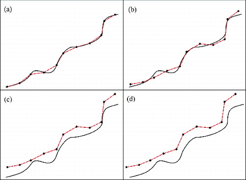
DTM accuracy is a vast topic, involving several error sources and figure 1 shows the main ones. Figure 1(a) shows the real terrain in black and the digital model in red; the DTM is a discretization of the terrain, thus presenting approximation errors, where the reconstructed surface significantly differs from the real one. Vertical noise is added in figure 1(b), while altimetric bias is further included in figure 1(c). Finally, figure 1(d) also shows the planimetric offset.

Figure1. DTM error sources. Subframe (a) shows the terrain (solid line) and the discretized digital model (dashed line). In (b) vertical noise is added. In (c) and (d) altimetric and planimetric biases are added, respectively.

3.2. The fundamental vertical accuracy condition

This paper doesn't deal with all the above-listed items, but only with fundamental vertical accuracy, which is defined by the NDEP guidelines and is considered the most important DTM accuracy figure. More precisely, our paper deals with fundamental vertical accuracy assessment, for which the following prescriptions are given in the quoted guidelines:

• detect and fix horizontal and vertical offsets (methodology is not indicated);

• measure a sufficient number of CKPs, 20 or more in open areas (no filtering problems) and where the terrain is flat or where the slope is limited and constant (no approximation problems).

As shown above, the NDEP guidelines neither specify the procedure for detecting and removing outliers, nor do they define the way to fix horizontal and vertical offsets. CKPs must be measured in open areas, to be sure that the DTM is not locally perturbed by mass points generated by trees or buildings. Finally, CKPs must be located on flat terrain or where the slope is limited and constant, in order to limit theeffect of the approximation error. This error describes the difference between the DTM discretized surface and the real one, independently of the existence of random errors (see figure 1(a)): it depends on surface roughness and DTM spacing. There are parts of the terrain that are similar to a plane, in which the terrain is flat or has a uniform slope. The approximation error vanishes on those parts, provided that TIN or bilinear interpolation is used. This is why the NDEP guidelines recommend measuring CKPs on such parts.

In summary, our discussion is on fundamental vertical accuracy assessment; it is assumed that outliers were removed and horizontal and vertical shifts fixed; it is also supposed that CKPs are located on open terrain or where the slope is uniform. All these prescriptions will be indicated from now as FVA (Fundamental Vertical Accuracy) condition.

3.3. Precision and accuracy

Before continuing our discussion, it is worth clarifying our use of the precision and accuracy terms. According to most of the literature (Wolf & Ghilani 1997), precision is the root mean square distance between measurements and their empirical mean, while accuracy concerns the root mean square distance between measurements and their true value. Precision is related to random errors, while accuracy also accounts for systematics.

3.4. The two vertical accuracy definitions

It has been anticipated that two DTM vertical accuracy definitions are conceivable, which are illustrated in figure 2; for the sake of clarity, we will now list all the items involved and name them:

Figure2. Location of the quantities considered; VAN and VPN exist in all the four nodes, but are only shown for one. Grid geometry is shown, but the figure can be very easily adapted to the TIN case.

• Vertical Accuracy at the Nodes (VAN): the average vertical distance between the nodes and the terrain;

• Vertical Precision at the Nodes (VPN, ): the standard deviation of random noise at the nodes;

• Vertical Accuracy at the interpolated Points (VAP): the average distance between the generic interpolated points and the terrain;

• Vertical Precision at the interpolated Points (VPP, ): the standard deviation of random noise at the generic P points.

3.5. How VAN and VAP are reduced when the FVA condition holds

VAN and VAP have in general a complex error budget; when the FVA condition holds, VAN and VAP are greatly simplified, as a result. Concerning VAN, when planimetric and altimetric biases are fixed, VAN only consists of VPN, which quantifies random errors and is more precisely described later. Concerning VAP, once biases are fixed, it is the sum of two items: VPP, which is the propagation of VPN, and the approximation error. Under the FVA condition, the approximation error vanishes and VAP coincides with VPP.

3.6. Rigorous statistical definition of the quantities involved

A precise statistical definition of the considered quantities is synthetically illustrated in figure 3. The height of each node is a random variable (RV) having a true value and a dispersion , corresponding to VPN; the four involved nodes have different mean values, , but the same standard deviation . The actual node height is an extraction from the RV ; all the are assumed to be uncorrelated; there are no specific assumptions on the statistical distribution of the RVs.

Figure3. The random variables involved.

A generic point is now considered: its height can be obtained from the nodes’ heights by interpolation. Bilinear and TIN interpolation methods are only considered here, as they are by far the most used methods for second interpolation (NDEP 2004). The interpolated height is another random variable , which is a function of the involved in the interpolation. Its standard deviation comes from variance propagation and can be formally evaluated, as the initial variance–covariance matrix (1) and the interpolation functions are known: bilinear and TIN. (1) Matrix (1) is related to the grid case, while, in the TIN case, the variance–covariance matrix would be , with the same structure.

3.7. Vertical accuracy assessment

The empirical assessment of DTM vertical accuracy is now considered. This task is usually performed by comparing the surface with a number of CKPs. Their true heights are and the corresponding DTM heights are indicated with . The latter can be obtained in two distinct ways, depending on the CKPs’ position. If they coincide with the DTM's nodes, the are already available. Otherwise, bilinear or TIN interpolation is applied. The differences can be evaluated(2)

Under the FVA condition, several error sources are eliminated and the empirical mean of the differences (2) is zero by hypothesis. Therefore, the empirical standard deviation can be simply estimated by (3) Two assessment schemas are now conceivable:

• when CKPs are randomly chosen, formula (3) is, according to statistics (Wolf & Ghilani 1997), the estimation of ;

• when CKPs coincide with nodes, equation (3) is an estimation of .

Depending on the choice of CKPs, two different accuracy quantities are estimated. The second possibility is only apparently difficult in practice: using NRTK GPS, for instance, one can navigate to the planimetric position of one node and then measure the corresponding terrain height. Furthermore, when a Reference DTM (RDTM) is available, it can be interpolated in order to obtain the true height of terrain at the nodes of the Investigated DTM (IDTM).

4. A simulated example

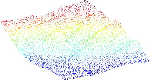
A simulated accuracy assessment experiment is carried out in this section. It is based on a real DTM (figure 4), created from spot heights and contour lines extracted from a 1:1,000 digital map of a city in Northern Italy. The nominal vertical tolerance (the largest admissible error) of the map is 0.60 m. The area considered has a size of 1,000 × 730 m² and contains 99,687 mass points, corresponding to an average inter-distanceof 2.65 m.

Figure4. The DTM used for the simulated assessment experiment. It was created from spot heights and contour lines extracted from a 1:1,000 digital map of a city in Northern Italy.

As previously explained, our paper discusses the different stochastical behaviour of the VAN and VAP quantities. This is also related to the fact that, when accuracy assessment is performed, the CKPs’ position matters. Before developing the formal and symbolic study of VAN and VAP (Section 5), it is worth inserting a numerical example, showing that different assessment strategies carry out significantly different results.

We underline that the goal of our study is not to discuss whether the data-set used is a good representation of the real terrain, as we only need a terrain-like model. From this point of view, we believe that the model shown in figure 4, extracted from a large-scale city digital map, is perfectly suitable.

To perform the simulation described, a set of Matlab procedures was created at the Geomatics Laboratory of the University of Pavia. A TIN model was calculated from the mass points extracted from the map and then two grid-based DTMs were created, having a cell size of 10 m and 1 m, respectively. A normally distributed random noise was added to the first one, having null mean and a standard deviation of 1 m, so that it represents a real DTM, containing measurement errors; we didn't add biases in order to be compliant with the FVA condition. In summary there are two grid-based DTMs:

• IDTM, the investigated DTM, having a cell size of 10 m and containing a random vertical noise of 1 m;

• RDTM, the reference DTM, having a cell size of 1 m and being error-free.

The IDTM vertical accuracy will now be assessed by comparison with 100 CKPs. These points have to be measured with some surveying technique, such as GPS NRTK. Therefore, 100 locations have to be selected and the corresponding heights measured. There are different options:

1. CKPs are randomly chosen among the IDTM's nodes;

2. CKPs are randomly distributed over the area covered by IDTM;

3. many other possibilities are conceivable, in line of principle; for instance: CKPs could be randomly chosen among the centres of IDTM cells.

Besides this, the latter two options require a further choice concerning the interpolation method by which the IDTM height is determined at the chosen CKPs. To reasonably summarize the available options, four assessment strategies are considered:

• S1 – CKPs are randomly chosen among the IDTM's nodes;

• S2 – CKPs are randomly distributed, so they can have any position inside cells; bilinear interpolation is used to obtain the IDTM height at the CKPs;

• S3 – CKP distribution is the same as S2, but TIN interpolation is used this time; even if a DTM has a grid structure, its regularly distributed nodes can be used to calculate a Delaunay triangulation and then perform TIN interpolation;

• S4 – CKPs have a peculiar distribution, because they are randomly chosen among the centres of IDTM cells; bilinear interpolation is used.

The first two columns of table 1 summarize the strategies considered. Within the frame of the present paper, CKP positions weren't physically measured, but obtained by interpolating RDTM, with our Matlab procedures. For the scope of our discussion, directly measuring CKPs on the terrain or obtaining them by interpolating RDTM are two equivalent procedures, as they both produce 100 points whose heights can be treated as true, with respect to IDTM.

Table1. The four considered assessment strategies and the estimated vertical accuracy.

Strategy	Methodology	Empirical STD [m]
S1	Check points at the nodes	0.96
S2	Check points randomly distributed; bilinear interpolation	0.71
S3	Check points randomly distributed; TIN interpolation	0.75
S4	Check points located in the centre of the cells; bilinear interpolation	0.48

After simulating all the necessary measurements and data, the differences were evaluated, following equation (2), and standard deviation was estimated, following formula (3). Results are shown in the third column of table 1. They all are vertical accuracy estimations of the same DTM, but are significantly different. Such differences certainly don't have a pure stochastic nature, because of their large size and the large sample number, equal to 100.

In detail, and following the previous discussion, S1 estimates VAN and indeed the resulting figure, 0.96 m is close to 1 m, which is the random noise inserted into IDTM in our simulation. S2 and S3 estimate VAP and show significantly lower values, 0.71 m and 0.75 m, respectively: this is empirical evidence that VAN and VAP don't coincide, due to error propagation. The difference between the S2 and S3 estimations is limited in size but hasn't a purely stochastical origin: Section 5 will highlight instead that TIN and bilinear interpolation have different error propagation properties, thus justifying such disparity. S4 is very interesting too: CKPs don't coincide with nodes, so the figure obtained, 0.48 m, is an estimation of VAP; but it is significantly different from those of S2 and S3. The explanation is given in Section 5: the noise contained in the interpolated height, calculated for a certain point, depends on its location within the DTM cell; it is minimal at the centre of the cell and takes higher values elsewhere. In S2 and S3, CKPs are randomly located; hence, the average noise of the interpolated height is estimated. In S4 CKPs are located at the centres of DTM cells, therefore, the minimum noise value of the interpolated height is estimated; the resulting empirical value, 0.48 m, is in good agreement with theory, illustrated in Section 5.

In conclusion, different results are obtained, when different assessment strategies are applied to the same DTM: the CKPs’ position matters. In other words, VAN and VAP, and their related quantities and , do not coincide. A theoretical study is needed now, to fully understand the statistical behaviour of VAN and VAP.

5. Error propagation in DTM second interpolation

The main results for error propagation in DTM second interpolation are summarized here. Bilinear and TIN interpolation methods are considered, which are the most used for DTM processing and analysis (NDEP 2004). The first is applicable to regular nodes only, and therefore solely to grid-structured DTMs, while the second can be applied to both TIN and grid structures. Results shown are rigorously obtained and don't contain any kind of approximation, due to the adoption of a Computer Algebra System (CAS), such as the Matlab Symbolic Toolbox.

5.1. Error propagation in bilinear interpolation

A square cell is considered in this section, having size d, whose lower left vertex is in the origin. Figure 5 shows the four nodes considered, their heights and the generic point. The interpolated height has the typical bilinear form(4)

Figure5. Bilinear interpolation.

and, imposing it to pass through the four nodes, the following analytical expression is obtained(5) At the centre of the cell is equal to the arithmetic mean of the four heights . The analytical expression for is also obtained(6)

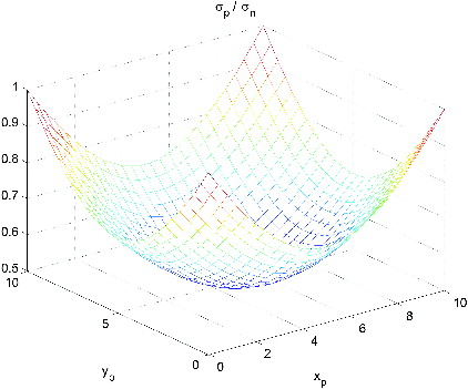
The function is not constant, meaning that the precision of the interpolated height depends on the position of the considered point within the cell. However, interestingly, the analytical expression of is independent from the nodes’ heights . In other words, it is independent from the terrain's morphology; the nodes’ heights can be all the same (flat terrain) or can take very different values (steep terrain), but this doesn't impact the value. Figure 6 shows the plot of the function : the minimum value is , at the centre of the cell, as the interpolated height is the simple mean of four independent measurements; the maximum value is 1, at the nodes.

Figure6. Plot of the ratio as a function of , for bilinear interpolation; cell size was set to 10 in order to produce the plot, but the function's shape is independent from .

As it is useful to have a single figure quantifying the average accuracy of the interpolated height over the whole cell, we introduce the parameter(7) It still depends on the position of the interpolated point within the cell, but can be easily averaged. The average quantities and can also be introduced, whose relationship is obtained by equation (7)(8) (9)

The average parameter can be calculated by a double integral(10) which, being a constant, is noticeably independent from and . The average standard deviation of the interpolated height is therefore, following equation (9)(11) In short, figure 6 shows that is not constant over the cell. Equation (11) states it is significantly lower than , being equal to two-thirds of it, on average, over the whole cell.

5.2. Error propagation in TIN interpolation

TIN interpolation is now studied. The considered triangle is shown in figure 7 and has one vertex in the origin and another one on the X axis.

Figure7. TIN interpolation.

The interpolated height is obtained by calculating the equation of the plane passing through the nodes , , and finding its height at the position :(12)

We showed before that bilinear interpolation has a special position in which the interpolated height is simply the arithmetic mean of the heights at the nodes; that position is the centre of the cell. Is there something similar for TIN interpolation? Indeed there is a notable point for which the function is equal to the arithmetic mean of the three heights , and that point is the mean position (centre from now) of the triangle, that is the point having coordinates(13) The analytical expression for is(14)

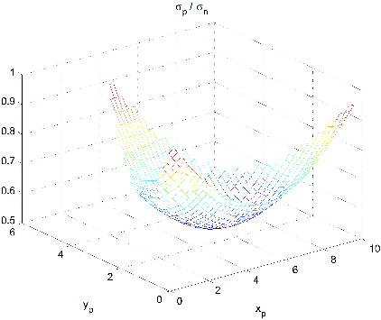
As for the bilinear case, is not constant and depends on the position of the interpolated point within the triangle, as equation (14) depends on and . Once again it is independent from the nodes’ heights, because equation (14) doesn't contain : this implies that error propagation is independent from the terrain's morphology. Finally, depends on the nodes’ planimetric coordinates (), so it is a function of the triangle's shape. Figure 8 shows the plot of the function : the minimum value is , at the centre of the triangle and the maximum value is 1, at the nodes.

Figure8. Plot of the ratio as a function of , for TIN interpolation. In order to produce the plot, the triangle having vertices , and was set, but the function's shape is independent from that.

The average coefficient is calculated(15) where the integration domain is the triangle. Noticeably, is a constant, so it is independent from the shape of the triangle and from . The average standard deviation of the interpolated height is therefore(16)

In short, figure 8 shows that is not constant over the triangle and equation (16) states it is significantly lower than , being equal to 0.71 of it, on average, over the whole triangle.

All results shown here refer to the triangle of figure 7 but have a general value; thanks to the symbolic capabilities of Matlab, we also tested the only other significant configuration, in which the node number 3 is positioned on the right of number 2; results are the same.

6. Discussion

The paper starts by stating that two DTM vertical accuracy definitions are conceivable:

• Vertical Accuracy at the Nodes (VAN);

• Vertical Accuracy at the interpolated Points (VAP).

These two quantities are not coincident and different numeric values are obtained, when they are calculated for the same DTM.

Section 4 shows an example. A DTM is created by simulation, having a grid structure and a random noise of 1 m at the nodes. Its vertical accuracy is estimated by means of 100 CKPs. These points can be chosen and measured according to several different strategies: four are depicted and summarized in the first two columns of table 1. The estimated standard deviations are reported in column 3 of the same table and highlight that CKP position matters. In other terms, VAN and VAP, and their related quantities and , do not coincide.

Finally, Section 5 performs a theoretical study of the statistical properties of VAN and VAP. When bilinear interpolation is used, the standard deviation of the interpolated height is, on average on the whole cell, (17) When TIN interpolation is adopted, the average standard deviation of the interpolated elevation is, on average on the whole triangle(18) Section 5 also shows that, when the interpolated height is evaluated at the centre of the cell, its standard deviation for grid-based DTMs, having squared cell, is (19)

Theoretical results expressed by equations (17), (18) and (19) are in strong agreement with the empirical findings of table 1. Remembering that, in the considered example, is 1 m, strategy S1 estimates VAN at 0.96 m, in good agreement with the true value. Strategy S2 gives an estimation of : the empirical figure is 0.71 m, while the theoretical one (17) is 0.67 m. S3 estimates : the empirical value is 0.75 and the theoretical one (18) is 0.71 m. For both S2 and S3, empirical results match the theoretical ones very well. Moreover, results (17) and (18) confirm that S3's estimate is slightly larger than S2's for conceptual reasons and not for noise. Finally, S4 quantifies and the estimated value, 0.48 m, matches the result (19) very well.

The four strategies studied are based on as many DTM vertical accuracy definitions. will no longer be considered, because it is singular and uncommon, although having the merit to show that error propagation plays a key role. Therefore, there are three remaining DTM vertical accuracies , and , which are significantly different and can't be interchanged. Two questions arise:

• which definition can be considered fundamental?

• How can we standardize empirical assessment procedures, in order to obtain comparable results?

First of all, we believe that VAN, accuracy at the nodes, must be considered the fundamental one, for a threefold reason:

• it is independent of the interpolation method used;

• it is not influenced by approximation issues;

• VAP can be obtained from it by variance propagation.

Concerning the second question, when empirical assessment is performed, three main scenarios can be conceived:

• CKPs coincide with nodes and can be estimated directly by means of formula (3);

• CKPs are randomly distributed and bilinear interpolation is used; equation (3) gives , but (the hat indicates an estimation of a certain quantity) can be obtained by (20)

• CKPs are randomly distributed and TIN interpolation is used; is estimated by equation (3), and is achieved by (21)

There is a final comment. Our whole discussion is conducted under the FVA condition: are our conclusions strictly suitable only in that frame or do they have a wider value? The FVA condition is explained in Section 3.2 and implies that VAN and VAP coincide with VPN () and VPP (), respectively. This is the most recommended condition under which DTM accuracy assessment should be performed, so we believe our discussion is fully significant.

If the assessment is performed generically, disregarding the FVA conditions, VAN and VAP don't simply coincide with VPN and VPP, but are the sum of several items. Nevertheless, two statements are still perfectly valid:

• VPN and VPP behave exactly as explained in our paper;

• VAN and VAP are different quantities and can't be interchanged.

7. Conclusions

The DTM vertical accuracy topic has been discussed; grid and TIN structures were considered, as well as bilinear and TIN interpolation. The discussion was conducted within the frame of the FVA condition.

Two vertical accuracy definitions are conceivable (Section 3): VAN (Vertical Accuracy at the Nodes) and VAP (Vertical Accuracy at the interpolated Points). These two quantities are not coincident and, when they are calculated for the same DTM, different numerical values are obtained: VAP is equal to approximately 70% of VAN, as shown in detail in Sections 4 and 5.

Furthermore, CKPs’ location plays a key role: when they coincide with the DTM's nodes, VAN is estimated; when they are randomly located, VAP is estimated instead (Section 4).

We believe that VAN must be considered the fundamental figure, for a number of reasons (Section 6); in other words, VAN is the vertical accuracy figure to be associated with a DTM to quantify its quality. When accuracy is empirically estimated, VAN can be directly estimated or, when VAP is estimated instead, suitable standardization coefficients must be applied to revert to VAN (Section 6).

Acknowledgements

The authors would like to thank the two anonymous reviewers for their careful reading of the paper and helpful comments. They have helped the authors to improve the quality and readability of the manuscript.

Vittorio Casella performed the analysis described in Section 5 and wrote Sections 5 and 6. Marica Franzini wrote Sections 2 and 8, prepared the data-set and performed the simulations of Section 4. The remaining parts of the paper were jointly written by both the authors.

Additional information

Funding

The authors acknowledge the partial financial support of the University of Pavia, Italy [FAR2012].

References

- Aguilar FJ, Mills JP, Delgato J, Aguilar MA, Negreiros JG, Perez JL. 2010. Modelling vertical error in LIDAR-derived digital elevation models. ISPRS J Photogrammetry Remote Sens. 65:103–110.
- Apel H, Merz B, Thieken AH. 2008. Quantification of uncertainties in flood risk assessments. Int J River Basin Manag. 6:149–162.
- Biagi L, Carcano L, Lucchese A, Negretti M. 2013. Creation of a multiresolution and multiaccuracy DTM: problems and solutions for a case study. Proceedings of the International Workshop The role of Geomatics in Hydrogeological Risk; 2013 Feb 27–28; Padua, Italy.
- European exchange circle on flood mapping. 2007. Handbook on good practices for flood mapping in Europe [Internet]. [ cited 2013 Sep 25]. Available from: http://ec.europa.eu/environment/water/flood_risk/flood_atlas/pdf/handbook_goodpractice.pdf
- Flood M. 2004. ASPRS guidelines - vertical accuracy reporting for lidar data. [Internet]. [ cited 2013 Sep 25] Available from: http://www.asprs.org/a/society/committees/standards/Vertical_Accuracy_Reporting_for_Lidar_Data.pdf
- Frey H, Paul F. 2012. On the suitability of the SRTM DEM and ASTER GDEM for the compilation of topographic parameters in glacier inventories. Int J Appl Earth Sci Geoinformation. 18:480–490.
- Fritsch D, Pfeifer N, Franzen M. 2013. Proceedings of the Workshop High Density Image Matching for DSM Computation. Official EuroSDR Publication No. 61.
- Giribabu D, Kumar P, Mathew J, Sharma KP, Krishna Murthy YVN. 2013. DEM generation using Cartosat-1 stereo data: issues and complexities in Himalayan terrain. Eur J Remote Sens. 46:431–443.
- Intergovernmental Committee on Surveying and Mapping. 2008. ICSM guidelines for digital elevation data: version 1.0; Aug. [Internet] [ cited 2013 Sep 25] Available from: http://www.icsm.gov.au/elevation/ICSM-Guidelines.pdf
- Kolecka N, Kozak J. 2013. Assessment of the accuracy of SRTM C- and X-B and high mountain elevation data: a case study of the Polish Tatra Mountains. Pure Appl Geophys. 170:1–16.
- Kraus K, Briese C, Attwenger M, Pfeifer N. 2004. Quality measures for digital terrain models. Int Arch Photogrammetry Remote Sens Geoinformation Sci. XXXV(B/2):113–118.
- Kraus K, Karel W, Briese C, Mandlburger G. 2006. Local accuracy measures for digital terrain models. Photogrammetric Rec. 21/16:342–354.
- Krieger G, Hajnsek I, Papathanassiou KP, Younis M. 2010. Interferometric synthetic aperture radar (SAR) missions employing formation flying. In: Proceedings of the IEEE. May; 98.
- Isaaks EH, Srivastava RM. 1989. An introduction to applied geostatistics. New York (NY): Oxford University Press.
- Liao M, Jiang H, Wang Y, Wang T, Zhang L. 2013. Improved topographic mapping through high-resolution SAR interferometry with atmospheric effect removal. ISPRS J Photogrammetry Remote Sens. 80:72–79.
- Maune DF. 2007. Digital elevation model technologies and applications: the DEM users manual. 2nd ed. Bethesta (MD): American Society for Photogrammetry and Remote Sensing.
- Mazzorana B, Huebl J, Fuchs S. 2009. Improving risk assessment by defining consistent and reliable system scenarios. Nat Hazards Hearth Syst Sci. 9:145–159.
- National Digital Elevation Program. 2004. Guidelines for digital elevation data: version 1.0; May 10 [Internet]. [ cited 2013 Sep 25]. Available from: http://www.ndep.gov/NDEP_Elevation_Guidelines_Ver1_10May2004.pdf
- Pirotti F, Guarnieri A, Vettore A. 2013. State of the art of ground and aerial laser scanning technologies for high-resolution topography of the earth surface. Eur J Remote Sens. 46:66–78.
- San BT, Suzen ML. 2005. Digital elevation model (DEM) generation and accuracy assessment from ASTER stereo data. Int J Remote Sens. 26:5013–5027.
- Shi WZ, Li QQ, Zhu CQ. 2005. Estimating the propagation error of DEM from higher-order interpolation algorithms. Int J Remote Sens. 26:3069–3084.
- Wolf PR, Ghilani CD. 1997. Adjustment computations: statistics and least squares in surveying and GIS. 3rd ed. New York: John Wiley & Sons.
- Zenger A. Smith DI, Hunter GJ, Jones SD. 2002. Riding the storm: a comparison of uncertainty modelling techniques for storm surge risk management. Appl Geography. 22:307–330.
- Zhu C, Shi W, Li Q, Wang G, Cheung TCK, Dai E, Shea GYK. 2005. Estimation of average DEM accuracy under linear interpolation considering random error at the nodes of TIN mode. Int J Remote Sens. 26:5509–5523.