Modelling and prediction of crop losses from NOAA polar-orbiting operational satellites

Abstract

Weather-related crop losses have always been a concern for farmers, governments, traders, and policy-makers for the purpose of balanced food supply/demands, trade, and distribution of aid to the nations in need. Among weather disasters, drought plays a major role in large-scale crop losses. This paper discusses utility of operational satellite-based vegetation health (VH) indices for modelling cereal yield and for early warning of drought-related crop losses. The indices were tested in Saratov oblast (SO), one of the principal grain growing regions of Russia. Correlation and regression analysis were applied to model cereal yield from VH indices during 1982–2001. A strong correlation between mean SO's cereal yield and VH indices were found during the critical period of cereals, which starts two–three weeks before and ends two–three weeks after the heading stage. Several models were constructed where VH indices served as independent variables (predictors). The models were validated independently based on SO cereal yield during 1982–2012. Drought-related cereal yield losses can be predicted three months in advance of harvest and six–eight months in advance of official grain production statistic is released. The error of production losses prediction is 7%–10%. The error of prediction drops to 3%–5% in the years of intensive droughts.

1. Introduction

Drought is a direct cause of famine killing hundreds of thousands of people and disrupting livelihood of millions in the developing countries (WFP 2014). The developed countries suffered from droughts as well due to an increase in the cost of population living following some shortages of food and price increase. From the most recent events, the droughts of 2010 in Russia and 2012 in the USA produced considerable local and global economic impacts. During the 2010, grain production in Russia dropped to 75 million metric tons (mmt) compared to 97 mmt in 2011. The 2012 drought in the USA costs the country's taxpayers nearly $35 billion in economic losses from considerable yield reduction, food and farmland price increase, water shortages, and fire-related ecosystem destruction. Both droughts have also led to global grain reduction, shortages of grain supply compared to the demands, lack of grain on the international market, and corresponding price increase (Goldenberg 2012; U.S. Drought 2012).

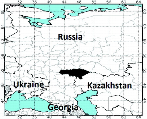
In the years when drought affects some of the major grain growing countries and regions (USA, China, India, European Union, Russia) global production falls below the consumption, the later has a high rate of increase due to a fast growing Earth population. In 8 of the first 13 years of the twenty-first century, global grain production falls below the consumption (PotashCorpo 2012). Therefore, assessment of drought-related losses of grain well in advance of harvest in the principal producing countries is an important task not only for that country but also for prediction of the global supply/demand, import/export, prices and evaluation of assistance to the developing nations. The goal of this paper is to investigate the potential of modelling commercial grain production of several grain crops (cereals) using space observations and estimation of drought-related losses of cereals in advance of harvest. Russia was selected for this experiment providing cereal production data and USA provided operational satellite data. Saratov oblast' (SO, administrative province) was selected as one of the important grain producing districts in the Lower Volga region located in the southeastern European Russia (figure 1).

Figure 1. Geographic location of Saratov oblast (SO), Russia: cereal crops are growing all over and VH satellite data were collected from the black area.

2. Grain in Russia and environment

Russia is the fourth largest grain producing country in the world after China, India, and USA. Grain harvested in Russia is entirely consumed inside the country. However, since the demands for grain are higher than the supplies, Russia purchases on the average nearly 3 million metric ton (mmt) of grain annually from the international market. In some years, when large-scale drought causes huge crop losses, this amount is doubled as it was in 1999 and 2000, when the purchases reached 7.8 and 5.8 mmt, respectively (FAO 2012). Therefore, advanced knowledge about the amount of grain collected in a particular year is very important not only for estimation of domestic grain use, but also projections of global supply and demand, international trade and consequently food security.

Southern Russia is the main grain basket in the country producing nearly 70% of high quality grain. Agricultural land of SO covers nearly 9 million hectares (ha), with 6.1 million ha occupied primarily with grain crops, which fields are traditionally huge and have not changed over years in order to receive maximum production with the best grain quality (Voeikov & Gortsev 2014; Zernoimport 2014). This region has fertile, well drained and nutritional Chernozem soils, which are good for cultivation of grain crops such as wheat, barley, oats, and corn. However, climate of this area is semi-arid, and the shortage of water puts considerable constraint on grain production. The situation is complicated by hot weather accompanied by desiccative winds (suhovei). Moreover, the unusually light snow cover does not make up for summer moisture deficit. Although this area has a few rivers, the area of commercial grain crops is so large that the amount of available water is not sufficient to offset dry climate. Therefore, grain crops are generally not irrigated. In drought years, up to 40% of grain production might be lost in that area.

One of the major geographic features of SO is Volga river, which divides the territory into two parts. The western part, (the right bank, of the river, excluding south), belongs to forest-steppe zone and the eastern part (the left river bank) belongs to steppe zone. The amount of grain produced each year in SO depends on the amount of natural water supply. Annual amount of precipitation (Pr) in SO is not large, changing from 500 mm in the north to 300 mm in the south. Most precipitation falls during the warm period. Moreover, since summer is hot, potential evapotranspiration (PET) in this area is large exceeding the amount of precipitation. As a result, the natural annual water balance (Pr-PET) is 200–400 mm short. Ninety per cent of this deficit occurred during warm period. The water shortage is usually accompanied by hot weather, droughts, and desiccative wind (suhovei). Droughts are typical for this region, affecting crops severely as it was in the past 30 years of the twentieth century (1972, 1975, 1980, 1984, 1995, and 1998). Light snow cover in this region does not offset the spring and summer moisture deficit (Kogan 1983).

Since climate controls grain losses, weather data are normally used for the modelling of individual grain crop production and prediction of losses. However, the weather-station network in Russia is not dense enough for accurate assessments of weather impacts, considering a very large area under grain, the number of farms growing crops, and high variability of rainfall. Moreover, since disintegration of the Soviet Union in the 1990s and deterioration of economic and social situation, the number of weather-observing stations in Russia reduced three times. Therefore, satellite data were used as proxy for weather variables in this area. These data were used before to model and monitor individual grain crops (wheat, corn, soybeans, and other) but have never been used for a group of crops, called cereals and grown in spring-summer (Liu & Kogan 2002; Dabrowska-Zielinska et al. 2002; Domenikiotis et al. 2004; Kogan et al. 2012).

3. Data

This study employs satellite and in situ data. In situ data were presented by production in tons (t), area in hectares (ha), and yield (Y, t/ha) for spring-planted cereals, which included wheat, barley, oats, corn, and pulses. Spring wheat, barley, and oats occupy 90% of the area. All crops are planted in late April early May and are harvested in August–September (USDA 1994). Therefore, cereal analysis in this research is represented by these three crops. The data were obtained from the Russia's Central Statistical Administration. Total regional production and area were summarized from the reports of all farms to SO level at the end of agricultural year; SO yield was calculated by dividing production by area.

Satellite data were collected from the National Oceanic and Atmospheric Administration (NOAA) Global Vegetation Index (GVI) data set during 1981–2012. Spatial and temporal data resolution was 16 km and 7-day composite, respectively (Kidwell 1997). Since grain crops occupy slightly over 6 million ha in SO, satellite data were aggregated from around 1100 (hundred times exceeding the number of weather stations used for spatial aggregation of SO precipitation and temperature) 16-km pixels in the SO area shown in figure 1. Such a large number of pixels are sufficient for characterizing average SO land cover conditions (Kogan et al. 2003). The GVI-based counts in the visible (VIS), near infrared (NIR), and infrared (channel 4, 10.3-11.3 µm) spectral regions were used in this research because they characterize conditions of vegetation, including crops. The first two changes with chlorophyll and water content in green vegetation and the last one helps to monitor thermal conditions. Pre-launch calibration was applied to VIS and NIR counts to convert them to reflectance, and post-launch calibration was applied to correct reflectance for sensor and orbit degradation (Kidwell 1997). Finally, these data were used to calculate normalized difference vegetation index (NDVI = (NIR - VIS)/(VIS + NIR)) and convert Ch4 counts to brightness temperature (BT).

4. Methodology

Both yield and satellite data time series were processed in the following way:

4.1. Yield

Yield time series of any crop over a period of more than 15 years can be approximated by the following equation (Obukhov 1949):(1) where Y_n is actual yield; Ŷ_n is a slow-changing yield's deterministic component controlled by the agricultural technology (breeding, mechanization, fertilizers, weeds control, etc.); dY_n is yield's random component regulated by weather fluctuation from year-to-year; n is the number of years in yield time series.

The technology-related yield trend (Ŷ_n) can be approximated by a polynomial (either linear or non-linear depending on longevity of yield series), regressing Y against year number. For yield time series longer than 20 years, non-linear polynomial approximation (for example, quadratic polynomial) is regularly used in order to represent appropriately the rate of yield growth and impacts of the interaction between climate and agricultural technology on yield (Fisher 1922; Obukhov 1949).

At a general background of the slow-moving technology-driven trend, fluctuations of yield around the trend are mainly explained by weather variations from year to year. In years of favourable weather for crop growth, yield exceeds the level estimated by the trend line and in the opposite situation of unfavourable weather yield drops below the trend. Following these considerations, dY_n is normally expressed as a ratio or difference (for a shorter time series). In this research, we used the ratio, characterizing deviation from agricultural technology related yield trend. This method allowed us to represent adequately variation of the yield around trend at the beginning and at the end of 20-year time series (Fisher 1922; Obukhov 1949).(2)

4.2. VH indices from the advanced very high resolution radiometer (AVHRR)

The principle for constructing these indices stems from the properties of green vegetation to reflect visible and emit thermal solar radiation. If vegetation is healthy, it reflects little radiation in the VIS part of solar spectrum (due to high chlorophyll absorption), much in the NIR part (due to scattering the light by leaf internal tissues and water content), and emit less thermal radiation in IR spectral bands (because the transpiring canopy is cooler). As the result, NDVI becomes large and BT small. Oppositely, for unhealthy vegetation NDVI becomes smaller due to reduced chlorophyll (less absorption and greater reflection) and water content (greater reflection) and BT larger because vegetation surface becomes hotter following reduced transpiration (Cracknell 1997).

It is important to emphasize that NDVI and BT quantify both spatial difference between productivity of different ecosystem (ecosystem component, EC) and weather-related variations in each ecosystem (weather component, WC). The EC is normally influenced by long-term environmental factors such as climate, soils, topography, landscape, geology, etc., while the WC is controlled by weather fluctuations in each ecosystem. Since weather-related NDVI and BT variations are much smaller than variations due to ecosystem differences, separation of WC (by calculating deviation of NDVI (BT) from their climatology) is an important procedure to do prior to comparing their each year weekly variations with each year yield fluctuations (Kogan 1997).

Following these considerations, the Vegetation health (VH) indices calculated from NDVI and BT were introduced. Details of the algorithm are presented in Kogan (1997). Here, the important steps are indicated. They include (a) complete elimination of high frequency noise from NDVI and BT annual time series, (b) approximation of annual cycle, (c) calculation of multi-year climatology, and (d) estimation of medium-to-low frequency fluctuations in NDVI and BT associated with weather variations (expressed as departures from seasonal cycle climatology). The VH indices were represented by NDVI-based Vegetation Condition Index (VCI), BT-based Temperature Condition Index (TCI) and Vegetation Health Index (VHI), aggregating VCI and TCI together. The equations (3(3) –5(5) ) provide these approximations.(3) (4) (5) where NDVI, NDVI_max, and NDVI_min (BT, BT_max and BT_min) are no noise (statistically smoothed) weekly NDVI (BT) and their 1982–2003 absolute maximum and minimum representing climatology of these indices, respectively; a is a coefficient quantifying a share of VCI and TCI contribution in the VHI. Since this share is generally not known for a specific location and time of the year, it was assumed that VCI and TCI contributions are equal (a = 0.5).

The values of these indices change from 0 to 100. Zero quantifies severe vegetation stress (moisture-based from VCI and thermal-based from TCI) associated with the lowest weekly NDVI (BT) values, which correspond to the 1982–2006 absolute minimum of weekly climatology (NDVI_min and BT_min). The VH value 100 quantifies very favourable conditions or the highest weekly NDVI (BT) corresponding to the 1982-2006 absolute maximum value of weekly climatology (NDVI_max and BT_max; Kogan 1995). The application of these indices as a weather proxy in a few countries (Poland, Brazil, Argentina, Zimbabwe, Morocco, Russia, India, Mongolia) showed that they correlate highly with productivity of crops and pastures and can be used as numerical weather indicators of agricultural losses in advance of harvest (Kogan 1997, 2002; Kogan et al. 2005; Liu & Kogan 2002; Dabrowska-Zielinska et al. 2002; Unganai & Kogan 1998). Weekly area-average indices (VCI, TCI and VHI) were calculated for the entire SO cereals growing area indicated in Atlas (1960) and USDA (1994). This area was inside the coordinates 42.5 − 51.5 N, 50.5 − 53.0 E. Mean values of VH indices were calculated from 1102 16-km pixels.

4.3. Statistical procedures

Since dY yield and VH indices were similarly expressed as a deviation from climatology (from trend for cereals and from max-min for VH), correlation and regression analysis were used to: select the index type, time of their strongest impacts on dY and develop dY-VH models to be used for assessment of yield losses. The data selected for statistical analysis included 20 years of cereal yield (derived after harvest time) and 20 years of VH data for 52 weeks in each year (total 1040 images were used to calculate mean spatial value of each index for the entire period). The Pearson correlation coefficients (CC) were used as a criterion to initiate this selection. Since the number of variables is large (considering three indices and 30-week intervals for each) and they are inter-correlated (collinear), two methods of variable (predictors in statistical model) reduction were applied (a) partial correlation coefficients (Snedecor 1965) and (b) weighting variable contribution and aggregating them to one variable following Obukhov (1949).

The partial correlation coefficients (PCC) method estimates the contribution of each independent variable when other variables are fixed at the average level (Snedecor 1965). The PCC indicator is an important criterion to use for the selection of predictors, which are collinear with others and have the largest contribution to variability of a dependent variable (predictant). Models, which include collinear variables, become statistically unstable and less accurate. In order to improve such model's stability, the variables with the lowest PCC should be removed. The procedure of predictors' selection consists of several steps. In the first one, a dY-VH model is built based on all weeks with the highest CC for a particular index. In the following steps, the predictors with the lowest PCC are removed and for the remaining predictors PCCs are re-estimated. This procedure is finalized when the remaining predictors have PCC ≥ 0.6.

After PCC-based predictors' selection is completed, the method (b) is applied: predictors from several weeks are aggregated into one variable with the weights calculated from CC values using approximation in equation (6(6) ). These weights are applied to the corresponding variable following equation (7)(7) , showing for VCI example.(6) (7)

In equations (6(6) ) and (7(7) ), W – weight, CC – correlation coefficient, CC² – determination coefficient, i and n – first and last weeks of predictors' aggregation, respectively, k – the new aggregated variable.

4.4. Validation

An important step in building statistical models is to test model predictions outside of a training set, because if the same training data set is used the results of model performance would be very optimistic due to instability of model (Snedecore 1965). Since the data sample used in this study is limited, a cross-validation technique was applied for independent model verification. In this approach, a single year was left out one-by-one from the data, a model was built for each set without one year and prediction was made for the removed year. The models were evaluated based on determination coefficient (R²) for predicted (P) versus observed (O) yield values, bias ((B) - difference between (P) and (O) yields), mean B (MB = (∑B)/N), relative bias ((RB) = 100*(B)/(O)), and Mean bios error (MBE = (∑(B)²/N), both systematic (SMBE) and non-systematic (NMBE). The SMBE and NMBE estimate what portion of MBE is unaccounted (due to predictors not included in the model) and accounted (due to included predictors), respectively (Willmott 1982).

5. Results

Figure 2 shows mean SO cereal yield (t/ha) and its linear trend during 1971–2001. The trend was approximated from the 10-year longer than modelling data set in order to avoid errors at the ends of shorter-period time series (Snedecore 1965). Following equation (1)(1) , trend was approximated as Ŷ_n = 1.08 + 0.000013*year; dY_n was estimated from equation (2)(2) . Average VCI, TCI, and VHI for SO area (USDA 1994) were calculated for each year of the 1982–2001 period from 1102 16-km pixels. It is important to mention that the time series of indices (not shown) did not experience any trend due to a comprehensive processing procedure applied to satellite data. Since these indices represent weakly deviation from their climatology for each year, they were further correlated with the mean SO cereal yield anomaly.

Figure 3 shows dynamics of the Pearson correlation coefficient for the end of season dY_n (the numbers for the collected yield are normally available in January–February of the year following crop harvesting) with the indices (upper) and with SO area mean total monthly precipitation (dP) and mean temperature (dT) anomaly. As seen, the dynamics for three indices and weather parameters is smoothed and indicates near zero correlation prior to crops planting and high correlation in the middle of the growing season.

Table 1 demonstrates five steps of predictors' selection for the dY_n – TCI and VHI models based on the PCC values. Principally, the lowest PCC are eliminated from the models (steps 1–4) and the final model is built when PCC > 0.6 for all predictors, which is shown in step 5. Table 1 results were used to develop four models with all predictors (equations (8)(8) and (9(9) )) selected in table 1 and cumulative predictors (equations (10)(10) and (11(11) )) following the equations (6(6) ) and (7(7) ) approximation. Finally, table 2 and figure 4 demonstrate independent models' validation following (Willmott 1982). Figures 5 and 6 illustrate drought area and intensity during 2010–2013. These years were unusual, especially 2010 with almost 100% drought area; in two other years, drought area was estimated at 40% but thermal stress in spring of 2013 covered almost 80% of SO area.

Table 1. Selection of TCI and VHI predictors for cereal's dY models based on partial correlation coefficients (PCC), Saratov oblast, Russia.

Index	Correlation type	Step	Tci22	Tci23	Tci24	Tci25	Tci26	Tci27	Tci28	Tci29
TCI	CC		0.71	0.72	0.74	0.72	0.69	0.58	0.47	0.75
	PCC	1	0.31	0.15	0.49	0.40	0.61	0.81	0.83	0.58
	PCC	2	0.66		0.51	0.42	0.61	0.81	0.85	0.62
	PCC	3	0.47		0.50		0.68	0.82	0.81	0.52
	PCC	4			0.30		0.79	0.81	0.80	0.70
	PCC	5					0.80	0.81	0.81	0.75
VHI			Vhi22	Vhi23	Vhi24	Vhi25	Vhi26	Vhi27	Vhi28	Vhi29
	CC		0.68	0.79	0.77	0.79	0.80	0.73	0.77	0.73
	PCC	1	0.04	0.03	0.15	0.10	0.79	0.70	0.59	0.73
	PCC	2	0.18		0.16	0.56	0.79	0.71	0.70	0.72
	PCC	3	0.18			0.59	0.80	0.73	0.68	0.72
	PCC	4				0.49	0.80	0.73	0.67	0.72
	PCC	5					0.80	0.77	0.71	0.75

Table 2. Statistics of an independent testing of cereal models (1982--2001), Saratov oblast, Russia.

	Model 11	Model 10	Model 9	Model 8
MB	−0.011	−0.002	0.006	0.008
MBE	0.061	0.064	0.072	0.078
SMBE	0.009(15%)	0.012(22%)	0.013(18%)	0.015(19%)
NMBE	0.052(85%)	0.042(78%)	0.057(82%)	0.063(81%)
R^.2	0.598	0.521	0.544	0.518

MB is Mean Bias between independently predicted (P) and observed (O) yields (t/ha).

MBE is Mean Bias Error of simulated yield, which includes, SMBE–Systematic MSE and NMBE–Non-Systematic MSE.

R² is square of CC between independently simulated P and O yields.

6. Discussion

6.1. Yield trend

The cereal trend (figure 2) indicates that from the 1970s, agricultural technology-related yield did not increase and remained at the level of 1.1 t/ha. This means that the technology applied to spring grain crops in SO does not stimulate yield growth. Some of the causes of long-term yield hiatus are deterioration of environmental resources (exhaustion of soil fertility, destruction of upper soil layer by heavy machinery, weeds in the fields, etc.) as the result of their uncontrollable exploitation over a long period of time, worsening of the economic situation, ill policies, etc. Besides, deficient agricultural technology, shortage of water, and frequent droughts limit agricultural production even more. At the background of flat yield tendency, weather-related fluctuations of yield around the trend (dY) remained large. As seen in figure 2, the extreme deviations of cereal yield from the trend in SO were in 1975 (below the trend) and 1978 (above the trend) with dY estimated fraction at 0.34 versus 1.98, respectively. These values can be interpreted as yield reduction by 66% in 1975 due to unfavourable weather (64% reduction in mean SO summer rainfall) and increase by 98% in 1978 due to favourable weather (48% above climatic norm of SO spatial mean summer rainfall (Dronin & Bellinger 2005)).

Figure 2. Cereal yield time series in SO, Russia during 1972–2001.

6.2. Correlation of dY with VH indices and weather variables

Figure 3 shows correlation coefficient (CC) dynamics of dY versus VCI (moisture condition), TCI (thermal condition) and VHI (vegetation health) between weeks 10 (mid-March) and 40 (end of October). Our interests were to (a) investigate the strength of this relationship and (b) whether the strongest correlation coincides with the cereals’ critical period (the period of the highest crops’ requirements to moisture and thermal conditions) and (c) if dY-VH correlation matches with dY-weather correlation (both time and intensity).

Figure 3. Dynamics of correlation coefficient for Saratov oblast's cereal yield departure from trend with (a) SO spatial mean VCI, TCI, and VHI and (b) with SO spatial monthly mean precipitation and temperature anomaly (deviation from climatic normal).

As seen in figure 3, in the early spring, which is cereals’ pre-planting, planting, and emergence (weeks 10–15, March–April), the correlation for all indices is near zero. It increases sharply during the green biomass accumulation in April and May (weeks 17–22). Thermal conditions during this period show much stronger correlation. It means that they play greater role because at the general background of year-to-year moisture deficit in SO, productivity of cereals depends much on air temperature: if weather is hot, crops become stressed thermally and the end-of-season production is reduced; oppositely, cooler weather stimulates higher production. The maximum correlation in figure 3 occurs in June–July (weeks 26–30) for VCI and early June (weeks 23–25) for TCI. The timing of these maximums coincides with the critical period of spring-planted cereals’ development when they experience enhanced sensitivity to weather conditions: yield is below trend for VH indices below 40 and above trend if VH > 60.

It is important to emphasize, that correlation with in situ data (departure from climatology of total monthly precipitation (dP) and mean monthly temperature (dT)) shows similar to satellite data results. Correlation coefficients' time series of dY versus dP and dY versus dT in figure 3 (Kogan 1986) are complimentary (in timing and strength of the correlation) to dY versus VH correlation dynamics. Differences in the sign of the correlation for temperature anomaly (negative) and TCI (positive) is because TCI was designed to reflect a reverse temperature scale (from high to low, equation 4(4) ), while in situ temperature reflect changes from low to high.

Although the correlation dynamics in figure 3 were in line with cereals’ response to weather, it should be indicated that even for the weeks of the highest correlation, VCI explained only 15%–30% of dY variance (CC = 0.36–0.41, table 1), for TCI from 35% to 50% (CC = 0.47–0.75). The relationship of yield anomaly with VHI was the strongest (figure 3 and table 1) explaining up to 64% of dY variance (CC = 0.68–0.80). The largest correlation of dY with VHI emphasizes the importance of combining VCI (moisture conditions) and TCI (thermal conditions) together even if their contribution to VHI was approximated as equal (equation 5(5) ).

Both methods (a) PCC and (b) equations (6(6) –7(7) ) were applied for selection of variables (predictors) for dY-VH regression models. Table 1 presents the 4–6 steps process of the method (a) for removing weekly predictors with the lowest PCC values from TCI and VHI models. For example, in the first step for TCI model, a regression equation was developed for all variables (weeks 22–29) with the highest CC (the top line for each index). The PCC values in the first step indicated that TCI23 has the lowest contribution (PCC = 0.15) to the model; this variable was removed from the model and PCC were re-estimated for the remaining variables. Similarly, in the following steps, PCC values indicated that TCI 25, 22, and 24 do not provide statistically significant contribution (PCC = 0.42, 0.47, and 0.30, respectively) as predictors of dY (due to their collinearity with other predictors) and they were removed from the models step-by-step. Finally, after the TCI24 (PCC = 0.30 in step 4) was removed from the model, the remaining variables (TCI26–TCI29) had the highest values of PCC (0.75–0.81). These variables were included in dY model, equation (8)(8) . Similarly, dY–VHI model in equation (9)(9) included VHI26–VHI29 variables (PCC = 0.71–0.80).

The estimates for equations (8)(8) and (9(9) ) are statistically significant: the models' Multiple CC (MCC) is large; 0.83 and 0.86, respectively, R² explains 69% and 74% of the dY variance, respectively, N is the number of data records, and DF is degree of freedom. The underlined variables and all MCC are statistically significant at 1% and the remaining at 5%.(8) (9)

Meanwhile, small DF values indicate that further reduction of variables in these equations is needed. Therefore, the method (b) was applied to equations (8(8) ) and (9(9) ). To improve the stability of regression coefficients (Snedecor 1965), the number of independent variables was reduced to one only resulting in the maximum DF. Following the transformation in equations (6(6) ) and (7(7) ), equations (8)(8) and (9(9) ) were re-written as:(10) (11)

The MCC, R², and DF in equations (10(10) ) and (11(11) ) are statistically sound, however, not much different from models (8(8) ) and (9(9) ). Therefore, at the final step, all equations (8)(8) –(11(11) )) were tested independently.

6.3. Independent validation

The statistics of an independent testing of (P) versus (O) cereal yield in SO is shown in table 2. Following R² and MBE values, the best models were (9(9) ) and (11(11) ), which are based on VHI variables (both weighted and non-weighted). This again emphasizes importance of combining together VCI (calculated from NDVI and estimating moisture conditions) and TCI (calculated from BT and estimating thermal conditions). Although the R² for these equations are slightly different, equation (11)(11) (weighted VHI) has 7% smaller systematic MBE (0.009 versus 0.012) and larger non-systematic error (0.052 versus 0.042), which is an important indicator of how good might be model performance. It is important to mention that in the best models SMBE should approach to zero while NMBE should approach to MBE (Willmott 1982).

Finally, two points should be emphasized: (a) the independently validated models (table 2) have relatively high R² (0.518–0.598), although it is smaller than the R² (0.69–0.81) from the equations (8)(8) –(11(11) ), what means that the R² alone cannot be considered as a complete and reliable indicator of a well-performing model; the MBE and especially SMBE should always be estimated for this goal; (b) in April 2013, we received additional Saratov cereal yield data for the period 2002–2012 (11 years) and tested equation (11)(11) during this completely independent period of simulation. As seen in figure 4, equation (11)(11) -based simulated P and observed cereal yield match quite well: R² = 0.611, MB = −0.029, MBE = 0.082, SMBE = 0.013 (16%), and NMBE = 0.069 (84%). The completely independent model verification showed quite similar to table 2 statistical evaluation.

Figure 4. Observed and independently simulated (equation 11(11) ) SO cereal yield during 2002–2012.

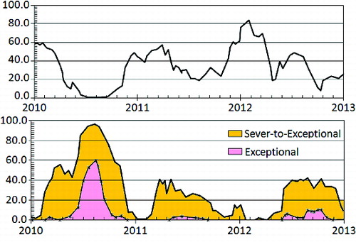
Losses of cereals were independently estimated quite accurately during 2010–2012, especially in 2010, when drought reduced cereal yield to 0.4 t/ha from the general trend level for that year of 1.2 t/ha (FAO 2012). Comparison of 2010-2012 droughts in European Russia is shown in figures 5 and 6. The drought of 2010 was high intensity and covered large area compared to other two years (figure 5). In the middle of summer of all three years, SO experienced thermal stress (TCI < 40). This stress was extreme in 2010 when TCI was below 20, for almost three months and near zero (exceptional intensity) for 1.5 months, while in the other two years the stress was weaker (TCI around 25) and shorter, continued less than two weeks (figure 6(a)). Thermal stress of severe-to-exceptional and exceptional (the strongest) intensity affected 100 and nearly 50% of SO area, respectively (figure 6(b)). In 2011 and 2012, the area of similar intensity thermal stress was much smaller

Figure 5. Drought area and intensity for the European Russia and western Kazakhstan in 2010–2012 (Rectangle indicates SO location).

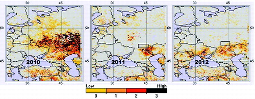
Figure 6. Saratov oblast VHI-based thermal stress dynamics (a) and per cent SO area under droughts of severe-to-extreme and exceptional intensity (b).

7. Conclusions

This paper discusses application of satellite-based globally universal VH technique, used originally to monitor VH and drought detection, for statistical modelling of crop yield. Previously this technique was applied and showed good results to model individual crops (wheat, corn, sorghum, rice, etc.). In this study, the VH proxies were applied to a combination of grain crops, called cereals, which included wheat, rye, barley, oats, corn, and pulses. The region was Saratov oblast, one of the major producers of grain in the southern European Russia. The developed models were quite accurate and reliable in prediction of cereal yield 3–4 months in advance of harvest and 6–8 months before official statistics of grain harvest is released. From the three indices characterizing moisture (VCI), thermal (TCI) and VHI conditions, the last two were very good predictors of cereal yield in SO, especially yield losses as it was in 2010. Further investigation of yield losses predictors might include combining satellite data with weather data, specifically during winter and early spring when vegetation is still dormant and the application of VH indices is limited. The VH indices and data are delivered every week to http://www.star.nesdis.noaa.gov/smcd/emb/vci/VH/index.php. They estimate and display global and regional vegetation health, moisture and thermal conditions, drought, and fire risk. They also discuss climate issues and VH utility in global observing system. Finally, this method will be considerably improved with observations from the new generation of operational satellite, called Suomi NPP (S-NPP) with many advanced sensors on board. The new Visible Infrared Imager Radiometer Suite (VIIRS) has started to provide radiance measurements with much higher spatial resolution (375 m) and four times more spectral bands (compared to its predecessor). Besides, VIIRS is currently providing exceptional data quality due to on board calibration of visible channels, narrow response function, sharper view and consequently, better quality NDVI, new vegetation indices (from mid to IR channels), and other products (net primary production, leaf area, vegetation fraction, and others).

Disclosure statement

No potential conflict of interest was reported by the authors.

References

- Atlas. 1960. Atlas of USSR agriculture. Moscow: Geodesi and Cartography.
- Cracknell AP. 1997. The advanced very high resolution radiometer. London, England: Taylor & Francis.
- Dabrowska-Zielinska K, Kogan F, Ciolkosz KA, Gruszczynska M, Kowalik W. 2002. Modeling of crop conditions and yield in Poland using AVHRR-based indices. Int J Remote Sensing. 23:1109–1123.
- Domenikiotis C, Spiliotopoulos M, Tsiros V, Dalezios NR. 2004. Early cotton yield assessment by the use of the NOAA/AVHRR derived vegetation condition index (VCI) in Greece. Int J Remote Sensing. 25(14): 2807–2819.
- Dronin NM, Bellinger EG. 2005. Climate dependence and food problems in Russia 1900-1990. Budapest: Central University Press.
- FAO. 2012. Crop production. Rome. Available from: http://faostat.fao.org/site/567/default.aspx#ancor
- Fisher RA. 1922. The goodness of fit of regression formulae and the distribution of regression coefficients. J Royal Statist Soc. 85:597–612.
- Goldenberg S. 2012. US drought could trigger repeat of global food crisis. Guardian [Internet]. [Accessed 2015 Apr 11]. Available from: http://www.theguardian.com/environment/2012/jul/23/us-drought-global-food-crisis
- Kidwell KB. 1997. Global vegetation index user's guide. Washington (DC): NOAA Tech. Rep., Department of Commerce; p. 65.
- Kogan FN. 1983. Soviet grain production: resource and prospects. Soviet Geography: Rev Trans. XXIV(9):631–661.
- Kogan FN. 1995. Droughts of the late 1980s in the United States as derived from NOAA polar orbiting satellite data. Bull Amer Meteor Soc. 76:655–668.
- Kogan FN. 1997. Global drought Watch from space. Bulletin Am Meteorol Soc. 78:621–636.
- Kogan F. 2002. World droughts in the New Millennium from AVHRR-based vegetation health indices. Eos. 83: 557–564.
- Kogan F, Gitelson A, Zakarin E, Spivak L, Lebed V. 2003. AVHRR-based spectral vegetation indices for quantitative assessment of vegetation state and productivity: calibration and validation. Photogrametric Eng Remote Sensing. 69:899–906.
- Kogan F, Salazar L, Roytman L. 2012. Forecasting crop production using satellite based vegetation health indices in Kansas, United States. Int J Remote Sensing. 3:2798–2814.
- Kogan FN, Yang B, Wei Guo. 2005. Modeling corn yield in China using AVHRR-based vegetation health indices. Int J Remote Sensing. 26(11):2325–2336.
- Liu WT, Kogan F. 2002. Monitoring Brazilian soybean production using NOAA/AVHRR based vegetation condition indices. Int J Remote Sensing. 23:1161–1179.
- Obukhov VM. 1949. Urozai I Meteorologicheskie Factoru (Yield and Meteorological Factors). Moscow: Gosplanizdat; p. 349. Russian.
- PotashCorpo. 2012. Agriculture: crop overview. [Accessed 2012 Nov 22]. Available from: http://www.potashcorp.com/industry_overview/2011/agriculture/16
- Snedecor GW. 1965. Statistical methods. Ames, IA: The Iowa State University; p. 534.
- USDA (United States Department of Agriculture). 1994. Major world crop areas and climate profile. Washington (DC): Agricultural Handbook, No. 664; p. 279.
- U.S. Drought. 2012. The New York times, science. [Accessed 2012 Dec 10]. Available from: http://topics.nytimes.com/top/news/science/topics/drought/index.html
- Unganai LS, Kogan FN. 1998. Drought monitoring and corn yield estimation in Southern Africa from AVHRR data. Remote Sensing Environ. 63:210–232.
- Voeikov VI, Gortsev AI. 2014. Saratov oblast. [Accessed 2014 Jul 15]. Available from: http://encyclopedia2.thefreedictionary.com/Saratov+Oblast
- [WFP] World Food Program. 2014. [Accessed 2014 Apr 5]. Available from: http://www.wfp.org/hunger/stats
- Willmott CJ. 1982. Some comments on the evaluation of model performance. Bulletin Am Meteorol Soc. 63:1309–1313.
- Zernoimport. 2014. Agriculture of Saratov region. [Accessed 2014 Jul 15]. Available from: http://zerno-import.ru/saratov_eng.php