A simplified early-warning system for imminent landslide prediction based on failure index fragility curves developed through numerical analysis

Abstract

Early-warning systems (EWSs) are crucial to reduce the risk of landslide, especially where the structural measures are not fully capable of preventing the devastating impact of such an event. Furthermore, designing and successfully implementing a complete landslide EWS is a highly complex task. The main technical challenges are linked to the definition of heterogeneous material properties (geotechnical and geomechanical parameters) as well as a variety of the triggering factors. In addition, real-time data processing creates a significant complexity, since data collection and numerical models for risk assessment are time consuming tasks. Therefore, uncertainties in the physical properties of a landslide together with the data management represent the two crucial deficiencies in an efficient landslide EWS.

Within this study the application is explored of the concept of fragility curves to landslides; fragility curves are widely used to simulate systems response to natural hazards, i.e. floods or earthquakes. The application of fragility curves to landslide risk assessment is believed to simplify emergency risk assessment; even though it cannot substitute detailed analysis during peace-time. A simplified risk assessment technique can remove some of the unclear features and decrease data processing time. The method is based on synthetic samples which are used to define the approximate failure thresholds for landslides, taking into account the materials and the piezometric levels. The results are presented in charts. The method presented in this paper, which is called failure index fragility curve (FIFC), allows assessment of the actual real-time risk in a case study that is based on the most appropriate FIFC. The application of an FIFC to a real case is presented as an example.

This method to assess the landslide risk is another step towards a more integrated dynamic approach to a potential landslide prevention system. Even if it does not define absolute thresholds, the accuracy is satisfactory for a preliminary risk assessment, and it can provide more lead-time to understand the hazard level in order to make decisions as compared with a more sophisticated numerical approach. Hence, the method is promising to become an effective tool during landslide emergency.

1. Introduction

Fragility functions or damage probability matrices are developed and used for determining structural capacities under loadings. They are conditional probability functions which give the probability of a structure to attain or to exceed a particular damage level for a load with a certain intensity level (Nateghi & Shahsavar 2004; Avşar et al. 2012). For example, in earthquakes they describe the relationship between the ground motion and the level of damage in a structure (Bommer et al. 2002; Rossetto & Elnashai 2003), but in flood risk management, it is the inundation depth and the consequential economic damage (Suppasri et al. 2011; Mas et al. 2012). Organizing vulnerability information in the form of fragility curves is widely adopted, when information is to be presented referring a multitude of uncertain factors (Stephenson & D'Ayala 2014), e.g. structural characteristics, soil–structure interaction, and site conditions particularly for the seismic hazard estimations (Shinozuka et al. 2000).

As a structural reliability concept, fragility curves have a long history originating first in seismic engineering (Casciati & Faravelli 1991). They have been common tools to make the seismic assessment of bridges' vulnerability as a function of ground motion intensity (Nielson & DesRoches 2007). Their use in flood risk management was first postulated by the US Army Corps of Engineers (USACE 1993) for economic assessments, but has not been widely adopted. They were taken up in the UK from 2002 when systems' analyses were introduced for national and regional flood risk assessments embodying the source-pathway-receptor concept (Simm 2010). Fragility curves then provided, together with levee overtopping assessments, the necessary pathway links (probability of levee failures) between the source hydraulic loadings and the receptor response in terms of flood depths and related financial impacts (Dawson & Hall 2002; Sayers et al. 2002; Hall et al. 2003).

Landslides are natural hazards, which include a wide range of ground movements, such as rock falls (Stock et al. 2012; Arosio et al. 2015), deep-seated slope failures (Jomard et al. 2014; Longoni et al. 2014) and shallow debris flows (Radice et al. 2012; Stoffel et al. 2014). Accordingly, landslides features can be grouped under three main concepts, (1(1) ) type of materials, (2(2) ) type of movements, and (3(3) ) velocity of failures (Varnes 1978; Cruden & Varnes 1996; Hungr et al. 2014), in which many uncertainties arise. It is costly and time-expensive to develop a comprehensive tool or method to define the movement states. The fragility curves have, conceptually, the ability to deal with uncertain sources while assessing risks in cost and time-efficient ways (Shinozuka et al. 2000). However, the adoption of the fragility curve theory to landslide risk assessment needs some practical upgrades in terms of development while following the conceptual theory. Shinozuka et al. (2003) emphasize the collective use of the following main principals to develop the fragility curves: (1(1) ) qualified, experienced based reasoning; (2(2) ) consistent and rational analysis; (3(3) ) calibration of the damage data with historic events; and (4) numerical simulation of structural response depend on dynamic analysis due to specific loadings.

There is a lack of studies on the vulnerability of elements in landslide risk assessment, which in turn hinder the use of fragility curves (Douglas 2007). Although expected damage to particular elements at risk can be determined for different types of mass movements based on different intensity scales or expert judgments (Cardinali et al. 2002; Bell & Glade 2004), majority of the current methods assume that the elements exposed to landslides will be completely destroyed (Glade 2003). The outcome of this case is a constant fragility curve equal to unity in the damage state. Nonetheless, within risk assessment for most other types of natural hazards, instead of fragility curves, the hazard levels are plotted. Such types of assessments provide qualitative guidance as to the level of risk due to a particular hazard but cannot be used to provide quantitative estimates of direct economic loss (Douglas 2007). Fragility curves might be adopted in this content in order to investigate the hazard level of a landslide related to the different states of a load.

The present study attempts to quantify the emergency states of landslides through fragility curves in real-time landslide risk assessments. This has been achieved by determining the response of a landslide to different piezometric levels (PLs) through numerical models. The information obtained is used to define, so called “failure indexes”, which are normalized forms of factors of safety (FS). Later on, they are visualized on the failure index fragility curves (FIFCs). Thus, the curves are used to assess the actual real-time risk on a real hazard which shares the same characteristics. Although the method presented was highly influenced by the fragility curve theory, whereas, it shares the same basic principles; it gives more of an indication about the current state of the landslide instead of an exceedance probability. The presented approach is based on process descriptions rather than on expert judgments and uses advanced numerical models based on the load variable of PL. Furthermore, the approach explicitly acknowledges the fact that a final slope failure is a consequence of a series of dependent parameters, so that the fragility curves for breaching processes can be combined to derive the final slope failure estimation subject to the given load. In turn it is convenient to be used as a preliminary landslide risk assessment tool in order to gain more lead-time in the case of an emergency.

The paper is structured as follows. In Section 2, we describe the theory of the FIFC technique together with how the model is developed to create it. The corresponding results are then compared and discussed in Section 3 with a real case (comprehensive numerical model). Section 4 contains the conclusion.

2. Method

2.1. Theory of failure index fragility curve (FIFC)

Two different sets of procedures describe how fragility curves are built. The first procedure is used when fragility curves are independently developed for different states of damage. The others are constructed progressively dependent on the previous state of damage. The empirical fragility curves are constructed exercising historical data obtained from past events (Vorogushyn et al. 2009). The analytical fragility curves are developed for typical exposed objects in a certain area based on nonlinear dynamic analysis (Jernigan & Hwang 2002; Negulescu & Foerster 2010). Although empirically developed fragility curves seem to be more convenient for landslide hazard assessment, it is not applicable considering the unique context (i.e. type of materials, depths of the sub-surface layers) of each landslide; which prevents a particular landslide to set an example to another landslide conceptually. On the other hand, tracing the movements of a landslide body for different PLs matches conceptually with the empirical fragility curve theory. Consequently, a deterministic analysis seems to be eligible to obtain the parameters to connect the PLs with landslide movements using a numerical model, an organigram is presented in Figure 1.

Figure 1. Organigram to illustrate the development steps of FIFC curves together with the application procedures.

Based upon this statement, the major effort is placed on the development of a fragility curve based on Shinozuka et al.'s (2003) 4th principal (described in the introduction); numerical simulations of the physical response of a landslide based on the dynamic analyses due to the rise or fall in the PL. Instead of a direct connection of the landslide movement to a change of the PL, normalized values are preferred. Dimensionless water index (W_i) and failure index (F_i) are normalized values computed, respectively, from the self-made simple equations (1)(1) and (2(2) ), from the FS and the PL. Normalization of these two terms allows the method to be implied in different real situations. Several curves are produced for each case to determine the propensity of a landslide to fail at a specific slope angle and material characteristics defined for a specific rock. The curves provide several options (slope angles vs. material characteristics) to help select the one for a specific need. Subsequently this can be used to develop the idea about the states of a landslide risk without the expertise of an experienced specialist.

First, W_i is calculated conditional on PL, which is the deepness of water from the surface and assumed equal along the slope by using the following equation(1) : (1) where PL_max is the maximum PL when FS = FS_dry (FS_dry is the FS in dry conditions) and PL_FS = 1 is the minimum PL implied in the model (when FS = 1) up to submerge conditions that is not included in the study.

After that F_i is easily estimated conditional to W_i by using the following equation: (2) where W_ic is the critical water index in which failure occurs (when FS = 1), and W_imin (in this study taken always as W_imin = 0) is the possible minimum water index (when PL = PL_max and FS = FS_dry). A sample demonstration of the FIFC is given in Figure 2.

As shown in Figure 2, the stability condition of a specific landslide sharing similar characteristics with the FIFC mentioned can be investigated. Only the piezometric reading from the field is needed. It is used to compute the W_i and, respectively, read the F_i, which is linked to W_i through the curve. Emergency phases can also be visualized on the curve associated with F_i in order to provide more information in the case of an emergency.

Figure 2. Schematic view of an FIFC.

2.2. Modelling features for deterministic analysis of FIFC

Considering that the aim of this study was to estimate the potential hazard level of a landslide, it was decided to focus more on the applicability and reliability than on the probabilistic analyses of the influencing parameters in fragility curve development. They are estimated by their influence on the sensitivity analyses of the porosity (p_t), the friction angle (ϕ) and the cohesion (c). The FIFC parameters (F_i, W_i) are specified deterministically through an analytical approach, instead of an empirical probabilistic approach, as this is generally the path in the development of a fragility curve. The parameters are obtained through a numerical model, which is developed with commercial software (Flac2D). The software determines the FS by the shear strength reduction (SSR) technique, instead of the traditional “limit equilibrium” method (LEM). The SSR technique is much more sensitive and reliable than the LEM. The SSR needs no artificial parameters, and it considers deformation of the elements. The LEM is based on equivalent forces (Dawson & Roth 1999; Cala & Flisiak 2001). Furthermore, The Mohr–Coulomb Failure Criterion is used by the software as expressed by the following equation(3) : (3) where τ is the shearing strength, σ is the normal stress and c is cohesion.

The input parameters c and ϕ are determined using the geological strength index (GSI). The GSI, introduced by Hoek and Brown (Hoek & Brown 1997) and largely adopted worldwide (Singh & Tamrakar 2013; Razmi et al. 2014; Eberhardt 2015) which could also be improved by semi-automatic innovative tool to investigate fractures (Longoni et al. 2012), is an estimation of the reduction in the rock mass strength for different geological conditions. Certain shareware software (i.e. RocLab, developed by Rocscience) is capable of providing c and ϕ for different GSIs of a specific material. Then the only remaining uncertainty is the FS obtained through the software conditional to the PL, which is initially given for each cycle to the model as the deepness of the water table from the surface.

2.3. Generic FIFC samples for early-warning system

Site conditions (the physical properties, the material and the material properties) are unique for each landslide. It is impossible to determine the incidence of different landslides only with one FIFC. Therefore, different slope angles and material characteristics for a given material are matched to represent various potential site conditions. Additionally, these FIFC input parameters are restricted to within some limits. Furthermore, the limits are carefully specified enabling them to be representative within a certain range.

Schist was selected as the surface material in order to ensure its match with the case study (see Section 3). Therefore, it is easy to assess the relevancy of the new method with a real case.

Material properties are given as the geologically-inferred c and the ϕ from the GSI. The slope and layer thickness are the geomechanical properties of a landslide. The material properties are particularly tested in order to grant the kinematics of the movement in the form of a Deep Seated Gravitational Slope Deformation (DSGSD) (Dramis & Sorriso-Valvo 1994; Arosio et al. 2013). It has been recognized that failure is more unlikely to occur in the form of a DSGSD for schist materials above a GSI value of 45 and, therefore, cases above this limit are neglected. GSI classes were selected from 0 to 45 in 3 major groups, 0–15, 16–30 and 31–45. With such values, surface conditions from fair to very poor and structures from blocky/disturbed/seamy to laminated/sheared are covered entirely within the GSI scale for jointed rock (Hoek & Brown 1997). The groups are representative for the given GSI intervals, but accuracy could be improved by reducing the size of the intervals.

Slope angles were grouped as 25°–35°, 36°–45° and 46°–55°. The slope inclinations were chosen to identify significant changes with the minimum number of FIFCs. However, sliding surfaces were chosen to be the worst cases, varying from 20 m to 50 m in all of the cases. Then, each GSI (c and ϕ) class was matched with all of the slope angles one by one to develop one FIFC. Finally, the thickness of the surface layer was selected to be 70 m to ensure that the sliding surface would remain in this layer only. Nonetheless, the bedrock was chosen to be strong enough to not have any influence on the results.

Nine FIFC curves were prepared in total and are presented in Figure 3. Each one embodies a specific condition performed by a single GSI range and a single slope angle range. All of the EWS phases are not visible in all the curves, whereas, the FS goes as low as 1.2 in the safest situation in some of the cases. This is because they were prepared to encompass all of the possible site combinations (GSI vs. slope angle). It is recognized that since the material strength is reduced, the failure occurs in the lower W_i rates. The same happens for the slope angle and for the higher W_i rates, as would be expected.

Subsequently, the curves are subjected to several sensitivity analyses. They are performed in the W_ic condition, with F_i = 1. The effects are recorded as absolute changes on the FS value and transformed into F_i, using equation (2)(2) . They are, then, cumulatively imposed on the curves in Figure 3 as error-bars to determine a range of uncertainty of F_i in the selected condition. First, the p_t values are increased from 0.04 up to 0.49 (Nicrosini 1987; EVS 1999; Barros et al. 2014). It is recognized that p_t has a relatively small influence on the FS (consequently on F_i) in the magnitude of 0.02 (Absolute) within the range from 0.24 and 0.38; while the results are more vulnerable to changes in the c and ϕ (see Table 1).

Table 1. Sensitivity analyses of FIFCs for different GSI groups ranging between 0 and 45.

GSI	pt (%)	FS	c (MPa)	FS	ϕ (°)	FS
0–15	0.04	1.00	0.05	0.96	15	0.94
	0.49	0.98	0.10	1.00	25	1.00
16–30	0.04	1.00	0.05	0.96	15	0.94
	0.49	0.98	0.15	1.00	25	1.00
31–45	0.04	1.00	0.09	0.98	20	0.95
	0.49	0.99	0.20	1.00	35	1.00

Cohesion (c) was tested incrementally from 0.05 MPa up to 0.20 MPa. Hoek (Hoek & Brown 1997) mentions that the c varies in the range of 0.09 MPa up to 0.18 MPa with GSI = 20 for schist, while ϕ is ∼22°. For a lower GSI (highly fractured surface with a disintegrated structure), c might decreases to 0.05 MPa with the ϕ from 15° to 18° (Chowdhury 1978). However, ϕ could go up to 35° for GSI≅40 (moderately weathered surface with a disturbed structure) with the c reaching 0.2 MPa (Chowdhury 1978; Hoek & Brown 1997). Consequently ϕ is tested in the ranges of ϕ = 15° to ϕ = 25° for GSI 0–30 and ϕ = 20° to ϕ = 35° for GSI 31–45. The significance of the effects are decreased in both cases for the higher degrees of ϕ (for GSI 0--30 above ϕ = 21° and for GSI 31–45 above ϕ = 29°). It was determined that ϕ influenced the FS in the magnitudes of 0.06 and 0.05 (absolute). Furthermore, c influenced the FS absolutely in the magnitudes of 0.04 for GSI 0–30 and 0.02 in for GSI 31–45.

Error-bars in Figure 3 contain significant information about the reliability of the method. Stability decreases while the slope angle (Dip) increases or the GSI decreases, the uncertainty in the curves rises proportionally. The potential error grows to a significant level since the stability conditions were reduced. Furthermore, the reliability of the method decreases along with the stability state. On the other hand, it provides information that emphasizes in such a condition the fact of an extremely unstable landslide situation.

Prediction of the landslide triggering thresholds is one of the key factors in the landslide research (Berardi et al. 2005), and the established thresholds are essential aspects in early-warning systems (EWSs) (Terlien 1998; Michoud et al. 2013). The landslide triggering thresholds differ from one region to another based on the hydro-climatological and the geomechanical properties, predominantly by the slope and the soil characteristics, the lithology and the morphology (Crosta 1998; Malamud et al. 2004; Capparelli & Versace 2014). Defining some phases of precise thresholds globally is difficult, while establishing warning thresholds is the main aim of landslide risk assessment science. The FIFCs would supply more information when the thresholds of each emergency phase are stated. An assumption of EWS phases was made to demonstrate the applicability of the effective FIFC. A threshold for the relevant phase was determined based on the curves already developed. It is presented in Table 2 based on the FS and can be correlated with Figure 3 by using the dash-dot-lines.

Table 2. Phases of EWS (2011 Lecture notes of S. Menoni; unreferenced).

FS range	EWS phase	Definition
1.30≤FS<1.40	Watching (green)	Activation of the emergency procedures
1.20≤FS<1.30	Warning alert (yellow)	Decision making
1.10≤ FS<1.20	Emergency (orange)	Implementation of the emergency measures
1.00 ≤ FS<1.10	Event (red)	Waiting for the event to happen

As it was described in Section 2.1, from Figure 3 a representative FIFC for the user's need can be selected and implied to a real case. The only parameter needed is the PL_max (FS = FS_dry) of the real case, which can be estimated with a simple numerical model of the slope, considering only the surface material. Then the W_i can be computed using the piezometric readings by using equation (2)(2) and F_i is determined associated to W_i from the curve together with the linked emergency phase. As a result a preliminary concept is obtained about the current state of the slope.

A group of FIFCs, which are generated for a GSI range 0–15, are merged into one single graph in Figure 4. The F_i values are projected respecting to the W_i values of the slope angle range of 25°–35° (the most stable case). In this case PL_min (= 0 m) and PL_max ( = 52 m) are determined for all three cases together, while it is determined individually for each of the singular FIFCs in the Figure 3. From Figure 4, the stability condition of a particular GSI class can be obtained for different slope angles. The slope influence is emphasized since, as expected, the steeper the slope, the lower the stability.

Figure 3. FIFC curves for schist; GSI values are sub-divided into three groups between 0–45 ranges, while slope angles (Dip) are also sub-divided into three groups between 25° and 55°. Related FS is given for each category in order to achieve the correlation with Table 2.

Figure 4. Early-warning stages for schist, GSI in the range of 0–15, slope angles rising from 25° up to 55°.

3. Application of the FIFC method to a real case

The FIFC method was applied to a landslide located in the northern Italy (Province of Lecco) on the extended side of the Mount Letè. The entire region is exposed to the risk of landslides because of the steep terrain and the continuous urban expansion. The municipality of Dorio is the principal vulnerable infrastructure, which lies at the foot of the landslide by Lake of Como. Following prolonged heavy rainfall, many slides developed into debris flows that have struck the town in the past, significantly in the summer of 1985 (Biasini 1996). Furthermore, the progressive retreat of the landslide's front is threatening the highway (SS36), which constitutes the main access route to the Valtellina Valley and the Swiss canton of Grisons from Milan and other cities in southern Lombardy, and some touristic facilities that were constructed on Mount Letè in recent years.

In the area, where the Mount Letè landslide took place, schists predominantly outcrop (Gianotti 1988) with the presence of gneiss increasing with depth (Cerro et al. 1994). The main schistosity is oriented in the East-West direction, locally towards slope with the dip angles ranging between 20˚ to 40˚. Two main families of discontinuity are recognized as well-oriented in the North–South and East–West directions. Both families are sub-parallel to the schistosity. This situation particularly characterizes the crown of a deep-seated landslide (Gianotti 1988). Additionally, most of the morphological structures and the fractures are giving decisive clues about a deep-seated landslide (Piccio & Nicrosini 1989; Biasini 1996).

Detailed properties of the soils involved are given in Tables 3 and 4 for the discovered three discovered subsurface layers based on the studies of Nicrosini (1987), Rossini (1991) and Cerro et al. (1994). Later on the findings of the Biasini (1996) confirm the work done previously. He emphasizes that although the materials quality changes from very poor to poor in the first 25 m, in the second 25 m the quality is increasing from fair to excellent according to the Rock Quality Index (RQD). He also defines a range of specific weights (dry) ranging from 26 and 29 kN/m³, while the majority is between 27 and 27.5 kN/m³ through the cracks around the crown.

Table 3. Physical properties of the layers determined by Nicrosini (1987), Rossini (1991), Cerro et al. (1994) and Biasini (1996).

Layers	Materials	Depth (m)	Structure	Surface conditions	Seismic velocity (m/s)
First	Schist	10–20 (≅15)	Heavily broken, intensely altered loose	Poor – very poor	500–800
Second	Schist–Gneiss	20–30 (≅25)	Fractured, faulted with angular blocks	Poor	1400–2000
Third	Gneiss	30–50 (≅40)	Blocky, almost undisturbed	Very good – Good	>3000

Table 4. Mohr–Coulomb strength parameters for the materials involved to the landslide determined through the studies of Nicrosini (1987), Cerro et al. (1994) and Biasini (1996).

Materials	Specific weight (γdry) (kN/m^3)	c (MPa)	ϕ (°)
Intensely altered schist	≅22.02	0.08	20
Fractured schist	≅27.25	0.21	27
Healthy gneiss	≅29.00	16.00	45

Some separated lake formations are recognized at this site: these phenomena are often called glacial fillings due to the presence of clay deposits that are not dominant in the area (Cerro et al. 1994). The presence of this clay is also seen at the foot of the landslide between 225 and 390 m above mean sea level (Gianotti 1988), and, subsequently, ignored in the analysis. However, the presence of perched water in the slope brings the question of seepage forces to mind together with the lake formations above the crown as the main triggering factor. Savazzi (1989) showed that there is no significant relationship between the water of the lakes above the crown and the springs downstream alongside the landslide site. Therefore, the piozemetric level is subjected to seasonal changes only (Piccio 1988; Biasini 1996).

3.1. 2D Numerical stability analysis of a water-induced landslide through a detailed model

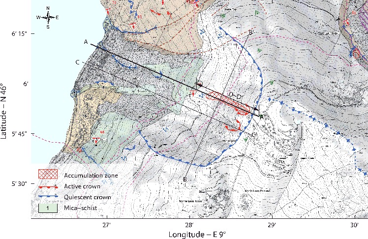
A two-dimensional numerical programme (Flac2D) was adopted for the case study. Four different cross-sections were determined considering the slope angle and the active crowns (see Figure 5). Section A-A', which had the highest slope angle and is presented in Figure 6, was used to quantify how the changes in the PL affected the stability of the slope, conceptually and quantitatively represented by the FS. Since the thicknesses of the layers were not precisely defined and changed slightly along the slope, a group of different combinations were analyzed. For the first layer they were selected as 10, 18 and 20 m, and for the second layer as 20, 27 and 30 m; while for the third layer it was always considered to be >50 m. Additionally the crowns (active and abandoned) were determined as detachment zones (Biasini 1996).

Figure 5. Layout of the Mount Letè (Invernizzi & Lambrugo 2005) with the selected cross-sections.

The model was calibrated based on the agreement of the movements detected by the monitoring devices (distance-meters, extensometers, crack-meters) with the piezometric data, which have been providing information since 1999 (ARPA 2014). Section D–D', where there is an active landslide accumulation, was used to determine critical limits of the PL. A majority of the tools were placed to determine the rates of movement caused by the crown cracks (ARPA 1999). Therefore, the reliability of this data is suspicious to calibrate a comprehensive model. Consequently, detailed sensitivity analyses were performed to emphasize the influence of the p_t, the ϕ and the c on the model.

The second and third layers had significantly higher resistance to the changes in the sensitivity parameters. Specifically p_t (from 0.00 to 0.20) had nearly no influence on either of the layers, while c (from 0.15 to 0.30 MPa) and ϕ (from 23° to 33°) had influence on the FS in the magnitude of 0.06 and 0.07 (Absolute), respectively, on the second layer. Even if the sliding surface almost never reached the third layer; when the two upper layers were at the minimum thickness, c (5–16 MPa) affected the FS in the magnitude of 0.04 (Absolute). This particular value was ignored in the model development referring to the parameters obtained from Table 4. Conversely, all of the sensitivity parameters had a higher magnitude of influence on the first layer. The ϕ angle (from 16° to 26°) influenced the FS significantly in the magnitude of 0.07, while c (from 0.07 to 0.10 MPa) in the magnitude of 0.05, and p_t (from 0.20 to 0.40) in the magnitude of 0.03; all of the values are absolute.

In the final stage, the model was used to investigate the relationship between the PL and the FS. This detailed model was developed to compare the results, hereby, obtained from it with the ones obtained from a selected FIFC curve. Critical stages were determined as; FS = 1 when PL = 10 and FS_max = 1.27 for PL_min = 35 m as demonstrated in equations (1)(1) and (2(2) ). In the light of the fact that the information obtained was projected onto an FIFC curve in Figure 7, left for this specific case (Mount Letè) only and named as FIFC_numeric.

Figure 6. Detailed plan of the A–A' cross-section with the view of the D–D' cross-section.

3.2. Implementing an FIFC to a real case and comparison with the comprehensive model

The use of an FIFC is rather simple, although their development requires the consideration of numerous uncertainties. However, after their generation, only a few criteria are required to select and apply the attributed curve to a real case.

First a simple model of the real slope should be developed and calibrated through visual field observations. The model should provide the needed information about the limits of PLs and the attributed FS together with the critical stages (FS = 1). Using equations (1)(1) and (2(2) ), the critical water index (Wic) and related failure index (Fi) can easily be calculated. Considering the surface conditions of Mount Letè, a simplified model can be developed with the slope angle 40° and GSI = 12. The limits states are given as; PL_max = 32 m, which is slightly lower than the comprehensive model, and PL = 10 m when the FS = 1. As long as the PL_min is taken as 0 m to create the FIFCs in Section 2, only the PL_max is needed to investigate the slope.

In the second stage a representative FIFC should be chosen for this specific case from the database of FIFCs, based on GSI and slope conditions of the real case. From there the emergency phase is based only on the piezometer readings. Consequently, slope angle variations and the surface material conditions of Mount Letè would direct us to the FIFC of GSI 0–15 and Dip 36°–45°, presented in Figure 7, on the right. Subsequently, a few different PLs would be used to get the FSs and the related emergency phase to compare with the real model of the slope in Figure 7, on the left.

To demonstrate: (1(1) ) With a PL of 20 m the information obtained from the selected FIFC is W_i = 0.38 (equation (1)(1) ), F_i = 0.35 (Figure 7, rights) and the FS = 1.18 (equation (2)(2) ). When the same PL is applied to the real numerical model the numbers obtained are W_i = 0.43 (equation (1)(1) ), F_i = 0.22 (Figure 7, left) and the FS = 1.21 (equation (2)(2) ). (2(2) ) With a PL of 13 m the information obtained from the selected FIFC is W_i = 0.59 (equation (1)(1) ), F_i = 0.70 (Figure 7, rights) and the FS = 1.08 (equation (2)(2) ). When the same PL is applied to the real numerical model, the numbers obtained are W_i = 0.62 (equation (1)(1) ), F_i = 0.64 (Figure 7, left) and the FS = 1.09 (equation (2)(2) ). The relative error between the comprehensive numerical model and the FIFC selected from the database is in the neighbourhood of 11%, which is satisfactory, and, meanwhile, cannot be completely ignored.

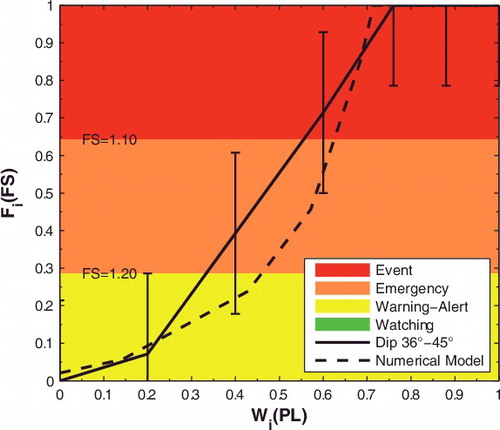
The FIFC (of GSI 0–15 and Dip 36°–45°) and the FIFC_numeric, respectively, are projected in Figure 8 to demonstrate a more detailed comparison. In dry conditions the results are highly correlated with each other. However, the correlation is relatively lower in the emergency phase. Close to the failure the trend re-converges and provides consistent results. Meanwhile, it should not be forgotten that the worst condition had been selected in creating the FIFCs. Therefore, it is acceptable that the results produced are nearly in agreement with the comprehensive numerical model. In contrast it provides a more unstable viewpoint. Additionally, the FIFC_numeric lies within the range limited by the error-bars of the selected FIFC. That is another significant indication that this novel approach is promising to be a strong tool of preliminary site investigation.

Figure 7. Left: FIFC generated considering the specific information obtained for the case Mount Letè (FIFC_Numeric). Right: Previously generated FIFC curve (GSI 0–15, Dip 36°–45°), which was selected to investigate the emergency phases at Mount Letè.

Figure 8. FIFC curve (GSI 0-15, Dip 36°–45°), which was selected to investigate the emergency phases at Mount Letè and the projected FIFC_numeric together with the related early-warning stages.

4. Conclusion

In many regions of the world, landslides cause high economic impact and often incur significant death rates (Keefer & Larsen 2007). In total more than 80.000 fatalities were recorded between 2002 and 2010 (2 May 2011 posting by D Petley to AGU Landslide Blog; unreferenced, see http://blogs.agu.org/landslideblog/2011/02/05/global-deaths-from-landslides-in-2010/). The numbers are dominated by the records from Asia, particularly around the Alpine-Himalayan Belt, followed by the ones from South and Central America. In such rugged terrain, the EWS becomes more crucial in preventing loss of life compared with structural measures, which are economically demanding. However, the design, applying, and operating a landslide EWS are multidimensional tasks and have rarely implied successfully (Huggel et al. 2010). Despite the attention given to decrease the number of uncertainties related to landslide-triggering conditions, which are obviously critical, most of the methods and techniques proposed are not equally cost-effective. More effort should be made to increase the economic efficiency, as well as the feasibility of these methods to provide more lead-time considering also the expertise level in the decision-making stage in the case of an emergency appears.

This paper presents an innovative method in the use of fragility curves for landslide risk assessment and for an EWS. Parameters influencing the stability conditions on a slope are investigated and different combinations of slope conditions are modelled through GSI values. For each combination an FIFC is produced to represent the evaluation of the movement defining the relationship between the geological components and the PL. FIFCs are developed deterministically through a numerical model and tested to determine their reliability in assessing an actual landslide, with a comprehensive sensitivity analyses.

The most significant advantage of the proposed method is its ability to evaluate landslide risk when only scarce data is available. Unless a comprehensive tool to assess the landslide risk exists, the FIFC can serve as a pre-early-warning-system. For the sites where conditions do not allow a detailed investigation of the slope, FIFCs could be used to determine the potential of a landslide hazard. Hence, due its systematic character the FIFC technique is promising to be used in the GIS applications. In addition, this method requires little expertise in identifying the state of the landslide danger and can be applied in the field by any staff member of an emergency centre.

Nevertheless, the results presented also indicate the necessity of further research to improve any globally-applicable landslide risk assessment method such as the FIFC. As illustrated in this paper, the fragility curves developed by the proposed technique perform satisfactorily compared to one exhaustively developed, but do not correlate fully. Thus, the consideration of landslide risk through the FIFC for civil security must be implemented as an interim solution. Further research and applications on different case studies with different geological and geomechanical conditions involved would contribute to the verification of the model in conjunction with monitoring systems to validate results on real landslide evolution (Scaioni et al. 2014; Calcaterra et al. 2015; Notti et al. 2015). Additionally the indexes (F_i, W_i) can potentially be improved by including the GSI parameters directly.

Acknowledgements

We gratefully acknowledge the Agenzia Regionale per la Protezione dell'Ambiente [Regional Environmental Protection Agency] (ARPA) for providing the opportunity to overcome an existing lack of knowledge in the field of landslide risk assessment by providing detailed data. Many thanks to Professor Dr Gianfranco Becciu, Mohamed Abdelhameed El Husseiny and Abdelaziz Mehaseb Elsayed Elganzory from Politecnico di Milano for their professional comments on our work and the support to convert the fragility curve theory to applications on landslide risk assessment. We would like to express our sincere appreciations to Dr Darwin Fox and Mr Andre Stettner-Davis from the University of Siegen helping to improve the quality of this paper.

Disclosure statement

No potential conflict of interest was reported by the authors.

References

- ARPA. 1999. Rete Geotecnica Manuale Frana Monte Letè: Provincia di Lecco Comune di Sueglio [Geotechnical Manual Network Crown of Mount Letè: Province of Lecco Municipality of Sueglio]. Dorio: (Agenzia Regionale per la Protezione dell'Ambiente) [Regional Environmental Protection Agency], Centro abitati instabili della provincia di Sondrio [Inhabited Unstable Centre of the Province of Sondrio].
- ARPA: Monte Letè (Monitorata dal CMG dal 1999): Scheda del dissesto “Monte Letè” [Mount Letè (Monitored by CMG since 1999): Board of instability “Mount Letè”] [Internet]. 2014: Italy: Agenzia Regionale per la Protezione dell'Ambiente [Regional Environmental Protection Agency]; [cited 2014 Mar 12]. Available from: http://cmg.arpalombardia.it/webcmgfrontend/dissesto.asp?def=39
- Arosio D, Brambilla D, Longoni L, Papini M, Zanzi L. 2013. New investigations to update the model of the premana (LC) landslide. In: Margottini C, Canuti P, Sassa K, editors. Landslide science and practice: risk assessment, management and mitigation. Berlin: Springer; p. 755–760.
- Arosio D, Longoni L, Papini M, Zanzi L. 2015. Analysis of microseismic activity within unstable rock slopes. In: Scaioni M, editor. Modern technologies for landslide monitoring and prediction. Berlin: Springer; p. 141–154.
- Avşar Ö, Yakut A, Caner A. 2012. Development of analytical seismic fragility curves for ordinary highway bridges in Turkey. Paper presented at: 15WCEE 24–28 Sep 2012. 15th World Conference on Earthquake Engineering; Lisbon (Portugal).
- Barros RS, Oliveira DV, Varum H, Alves CA, Camões A. 2014. Experimental characterization of physical and mechanical properties of schist from Portugal. Construct Build Mater. 50:617–630.
- Bell R, Glade T. 2004. Quantitative risk analysis for landslides ‒ Examples from Bíldudalur, NW-Iceland. Nat Hazards Earth Syst Sci. 4:117–131.
- Berardi R, Mercurio G, Bartolini P, Cordano E. 2005. Dynamics of saturation phenomena and landslide triggering by rain infiltration in a slope. In: Hungr O, Fell R, Couture R, Eberhardt E, editors. Landslide risk management. Proceedings of the International Conference on Landslide Risk Management; 2005 Jun 3. Vancouver (Canada).
- Biasini A. 1996. Il Monitoraggio dei Movimenti Franosi: Studio delle Frane di Spriana (SO) e del Monte Letè: Tesi Sperimentale di Laurea in Scienze Geologiche [The Landslide Movement Monitoring: Study of Spriana Landslide and Mount Letè Dissertation in Geological Sciences] [dissertation]. Pavia: University of Pavia.
- Bommer J, Spence R, Erdik M, Tabuchi S, Aydinoglu N, Booth E, del Re D, Peterken O. 2002. Development of an earthquake loss model for Turkish catastrophe insurance. J Seismol. 6:431–446.
- Cala M, Flisiak J. 2001. Slope stability analysis with FLAC and limit equilibrium methods. In: Billauax D, Xavier R, Detournay C, Hart R, editors. FLAC and numerical modeling in geomechanics. Proceedings of the second International FLAC Symposium; 2001 Oct 31. Lyon (France).
- Calcaterra S, Gambino P, Borrelli L, Muto F, Gullà G. 2015. Landslide activity and integrated monitoring network: The greci slope (Lago, Calabria, Italy). In: Lollino G, Giordan D, Crosta GB, Corominas J, Azzam R, Wasowski J et al., editors. Engineering geology for society and territory – volume 2: landslide processes. Cham: Springer; p. 1065–1068.
- Capparelli G, Versace P. 2014. Analysis of landslide triggering conditions in the Sarno area using a physically based model. Hydrol Earth Syst Sci. 18:3225–3237.
- Cardinali M, Reichenbach P, Guzzetti F, Ardizzone F, Antonini G, Galli M, Cacciano M, Castellani M, Salvati P. 2002. A geomorphological approach to the estimation of landslide hazards and risks in Umbria, Central Italy. Nat Hazards Earth Syst Sci. 2:57–72.
- Casciati F, Faravelli L. 1991. Fragility analysis of complex structural systems (1st ed.). New York (NY): Research Studies Press.
- Cerro A, Gianotti R, Perotti C, Piccio A, Savazzi G. 1994. La frana attiva del Monte Letè nel contesto della deformazione gravitativa pro-fonda di Dorio (LC) [The active landslide of Mount Letè in the context of pro-founded gravity deformation Dorio (LC)]. Atti Tic Sc Terra. 37:195–214.
- Chowdhury R. 1978. Slope analysis: developments in geotechnical engineering. Amsterdam: Elsevier.
- Crosta G. 1998. Regionalization of rainfall thresholds: an aid to landslide hazard evaluation. Environm Geol. 35:131–145.
- Cruden DM, Varnes DJ. 1996. Landslide types and processes. In: Turner AK, Schuster RL, editors. Landslides: investigation and mitigation. Washington (DC): National Academy Press; p. 36–75.
- Dawson EM, Roth WH. 1999. Slope stability analysis with FLAC. In: Detournay C, Hart RD, editors. FLAC and numerical modeling in geomechanics. Proceedings of the International FLAC Symposium on Numerical Modeling in Geomechanics; 1999 Sep 9; Minneapolis (MN).
- Dawson R, Hall J. 2002. Improved condition characterisation of coastal defences. In: Allsop, NWH, editor. Breakwaters, coastal structures and coastlines. Proceedings of the International conference organized by the Institution of Civil Engineers; 2001 Sep 28; London (UK).
- Douglas J. 2007. Physical vulnerability modelling in natural hazard risk assessment. Nat Hazards Earth Syst Sci. 7:283–288.
- Dramis F, Sorriso-Valvo M. 1994. Deep-seated gravitational slope deformations, related landslides and tectonics. Eng Geol. 38:231–243.
- Eberhardt E. 2015. The Hoek–Brown Failure Criterion. In: Ulusay R, editor. The ISRM suggested methods for rock characterization: testing and monitoring 2007-2014. Cham: Springer; p. 233–240.
- EVS: Effective Porosity: Total Porosity [Internet]. 1999. Lemont: environmental science division; [cited 2012 Aug 10]. Available from: http://web.ead.anl.gov/resrad/datacoll/porosity.htm
- Gianotti R. 1988. Relazione Geologica di Sintesi: Relazione Geologica di Monte Letè [Geological Report Summary: Geological Report of the Mount Letè]. Dorio (Italy): Comune di Dorio [Municipality of Dorio].
- Glade T. 2003. Vulnerability assessment in landslide risk analysis: vulnerabilitätsbewertung in der Naturrisikoanalyse gravitativer Massenbewegungen [Vulnerability assessment in natural risk analysis of gravitational mass movements]. Landslide hazard – Vulnerability assessment – Risk analysis. Die Erde. 134:123–146.
- Hall JW, Deakin R, Rosu C, Chatterton JB, Sayers PB, Dawson RJ. 2003. A methodology for national-scale flood risk assessment. Proc ICE - Water Maritime Eng. 156:235–247.
- Hoek E, Brown E. 1997. Practical estimates of rock mass strength. Int J Rock Mech Mining Sci. 34:1165–1186.
- Huggel C, Khabarov N, Obersteiner M, Ramírez JM. 2010. Implementation and integrated numerical modeling of a landslide early-warning system: a pilot study in Colombia. Nat Hazards. 52:501–518.
- Hungr O, Leroueil S, Picarelli L. 2014. The Varnes classification of landslide types, an update. Landslides. 11:167–194.
- Invernizzi P, Lambrugo M. 2005. Geology map, Componente geologica, idrogeologica e sismica del Piano di Governo del Territorio [Geological component, hydrogeological and seismic plan of the Territory] [map]. Dorio (LC): Commune di Dorio. 57 sheet: 1:10,000; digital; color.
- Jernigan JB, Hwang H. 2002. Development of bridge fragility curves. Paper presented at: 7th U.S. National Conference on Earthquake Engineering. Mira Digital Publishing; Boston, USA.
- Jomard H, Lebourg T, Guglielmi Y. 2014. Morphological analysis of deep-seated gravitational slope deformation (DSGSD) in the western part of the Argentera massif. A morpho-tectonic control? Landslides. 11:107–117.
- Keefer DK, Larsen MC. 2007. Geology: assessing landslide hazards. Science. 316:1136–1138.
- Longoni L, Arosio D, Scaioni M, Papini M, Zanzi L, Roncella R, Brambilla D. 2012. Surface and subsurface non-invasive investigations to improve the characterization of a fractured rock mass. J Geophys Eng. 9:461–472.
- Longoni L, Papini M, Arosio D, Zanzi L, Brambilla D. 2014. A new geological model for Spriana Landslide. Bull Eng Geol Environ. 73:959–970.
- Mas E, Koshimura S, Suppasri A, Matsuoka M, Matsuyama M, Yoshii T, Jimenez C, Yamazaki F, Imamura F. 2012. Developing Tsunami fragility curves using remote sensing and survey data of the 2010 Chilean Tsunami in Dichato. Nat Hazards Earth Syst Sci. 12:2689–2697.
- Malamud BD, Turcotte DL, Guzzetti F, Reichenbach P. 2004. Landslide inventories and their statistical properties. Earth Surf Process Landforms. 29:687–711.
- Michoud C, Bazin S, Blikra LH, Derron M, Jaboyedoff M. 2013. Experiences from site-specific landslide early warning systems. Nat Hazards Earth Syst Sci. 13:2659–2673.
- Nateghi FA, Shahsavar VL. 2004. Development of fragility and reliability curves for seismic evaluation of a major prestressed concrete bridge. Paper presented at: 13 WCEE .13th World Conference on Earthquake Engineering; Vancouver (Canada).
- Negulescu C, Foerster E. 2010. Parametric studies and quantitative assessment of the vulnerability of a RC frame building exposed to differential settlements. Nat Hazards Earth Syst Sci. 10:1781–1792.
- Nicrosini R. 1987. Studio Geologico Tecnico del Movimento Franoso del Monte Letè (Como) [Study of the technical geology of the Landslide Mount Letè (Como] [dissertation]. Pavia: University of Pavia.
- Nielson BG, DesRoches R. 2007. Seismic fragility methodology for highway bridges using a component level approach. Earthquake Engng Struct Dyn. 36:823–839.
- Notti D, Meisina C, Zucca F, Colombo A, Paro L. 2015. Map and monitoring slow ground deformation in NW Italy using PSI techniques. In: Lollino G, Manconi A, Guzzetti F, Culshaw M, Bobrowsky P, Luino F, editors. Engineering geology for society and territory: urban geology, sustainable planning and landscape exploitation. Cham: Springer; p. 141–145.
- Piccio A. 1988. Le glissement du Monte Letè [The slide of the Mount Letè]. In: Bonnard C, editor. Glissements de terrain [Landslides]. Proceedings of the Fifth International Symposium on Landslides 1988 Jul 15; Lausanne (Switzerland).
- Piccio, A, Nicrosini, R. 1989. Le condizioni di stabilità della nicchia di frana al Monte Letè, Suolo Sottosuolo [The stability conditions of the crown cavity of the landslide Mount Letè, Soil Basement]. Paper presented at: Suolo Sottosuolo [Underground Soil]. Congresso internazionale di geoingegneria [International Congress of geoengineering]; Torino (Italy).
- Radice A, Giorgetti E, Brambilla D, Longoni L, Papini M. 2012. On integrated sediment transport modelling for flash events in mountain environments. Acta Geophysica. 60:191–213.
- Razmi ZN, Lashkaripour GR, Ghafoori M. 2014. Geotechnical assessment and classification of ultrabasic rock masses in the South of Mashhad based on GSI and RMi classification systems. Int J Adv Earth Sci. 3:61–72.
- Rossetto T, Elnashai A. 2003. Derivation of vulnerability functions for European-type RC structures based on observational data. Eng Struct. 25:1241–1263.
- Rossini F. 1991. Relazione Tecnica sui Sondaggi Geognostici Eseguiti Press il Contiere Edilvie in Sommafiume di Sueglio (LC) [Technical report on drilling geognostic Performed At The Construction Site in Sommafiume of Sueglio (LC)]: Sondaggi no [Drill No]: S1-S2-S3-S4-S5-E1-E2-E3-E4-E5. Dorio: Comune di Dorio.
- Savazzi G. 1989. Indagine idrogeologica mediante l'impiego di traccianti (fluoresceina sodica), nell'ambito degli studi per il consolidamento dell'area del Monte Letè, a prote-zione dell'abitato di Dorio (LC) [Hydrogeological investigation through the use of tracers (sodium fluorescein), for the studies on the consolidation of the area of Mount Letè, the protection in the town of Dorio (LC)]. Dorio: Ministeriale della Protezione Civile [Ministry of Civil Protection] n.1259 FPC/TER 18/11/1987.
- Sayers PB, Hall JW, Meadowcroft IC. 2002. Towards risk-based flood hazard management in the UK. Proceedings of the ICE - Civil Engineering. 150:36–42.
- Scaioni M, Longoni L, Melillo V, Papini M. 2014. Remote sensing for landslide investigations: an overview of recent achievements and perspectives. Remote Sensing. 6:9600–9652.
- Shinozuka M, Feng MQ, Kim H, Uzawa T, Ueda T. 2003. Statistical analysis of fragility curves: technical report. Los Angeles (CA): University of Southern California.
- Shinozuka M, Feng MQ, Lee J, Naganuma T. 2000. Statistical analysis of fragility curves. J Eng Mech. 126:1224–1231.
- Simm J. 2010. Fragility curves and their use in UK flood risk management. Paper presented at: From Theory to Practice International Flood Risk Management Approaches (USACE); Washington (DC).
- Singh JL, Tamrakar NK. 2013. Rock mass rating and geological strength index of rock masses of Thopal-Malekhu river areas, central Nepal lesser himalaya. Bull Dept Geol. 16:29–42.
- Stephenson V, D'Ayala D. 2014. A new approach to flood vulnerability assessment for historic buildings in England. Nat Hazards Earth Syst Sci. 14:1035–1048.
- Stock GM, Martel SJ, Collins BD, Harp EL. 2012. Progressive failure of sheeted rock slopes: the 2009-2010 Rhombus Wall rock falls in Yosemite Valley, California, USA. Earth Surf Process Landforms. 37:546–61.
- Stoffel M, Mendlik T, Schneuwly-Bollschweiler M, Gobiet A. 2014. Possible impacts of climate change on debris-flow activity in the Swiss Alps. Climatic Change. 122:141–155.
- Suppasri A, Koshimura S, Imamura F. 2011. Developing tsunami fragility curves based on the satellite remote sensing and the numerical modeling of the 2004 Indian Ocean tsunami in Thailand. Nat Hazards Earth Syst Sci. 11:173–189.
- Terlien MTJ. 1998. The determination of statistical and deterministic hydrological landslide-triggering thresholds. Environm Geol. 35:124–130.
- USACE (U.S. Army Corps of Engineers). 1993. Reliability assessment of existing levees for benefit determination: engineering and design, technical letter 1110-2-328. Washington (DC): USACE.
- Varnes DJ. 1978. Slope movement types and processes. In: Schuster RL, Krizek RJ, editors. Landslides, analysis and control, Special Report 176. Washington (DC): National Academy of Sciences. p. 11–33.
- Vorogushyn S, Merz B, Apel H. 2009. Development of dike fragility curves for piping and micro-instability breach mechanisms. Nat Hazards Earth Syst Sci. 9:1383–1401.