Control-volume-based finite element modelling of liquefaction around a pipeline

Abstract

Pipelines are generally used to transmit energy sources from production sources to target places. Buried pipelines in saturated deposits during seismic loading could damage from resulting liquefaction due to accumulative excess pore-water pressure generation. In this paper, the evaluation of liquefaction potential in the vicinity of an offshore buried pipeline is studied using the control-volume-based finite element method. The objective of the present work is to study the effect of different governing parameters such as the specific weight of pipeline, Poisson's ratio, permeability of the soil, deformation module, pipeline diameter and pipeline burial depth on the soil liquefaction around a marine pipeline. The results of analysis indicated that with the increase of deformation module, Poisson's ratio and permeability of the soil coefficient, the liquefaction potential reduces. The liquefaction potential around the gas pipeline is much more than oil pipeline.

1. Introduction

Submarine pipelines have been extensively used for transportation of gas and crude oil from offshore platforms, disposal of industrial and municipal waste into the sea, and for cooling water in power plants. One of most important geotechnical considerations for many engineering structures, such as anchors and pipeline, is the potential sand deposits’ instability due to the development of high excess pore pressure caused by seismic loading (Chou et al. 2001). During the recent earthquakes such as 1995 Kobe, Japan earthquake, the 1999 Chi-Chi, Taiwan earthquake, the 1999 Kocaeli and Duzce, Turkey earthquakes, some underground structures experienced some damage were also of concern (Hashash et al. 2001; Wang et al. 2001; Rezaei et al. 2015; Tavakoli & Kutanaei 2015; Sarokolayi et al. 2015; Unutmaz 2014). During an earthquake, soil particles are subjected to alternating cycles of shear stress of randomly varying magnitude. In cohesionless soils and composite soils with cohesive fines, the soil structure tends to decrease in volume in response to the application of cyclic strains. Lack of drainage due to low permeability and short cycles of loading results in a nearly undrained condition. No decrease in volume can occur if the sand deposit is undrained, and thus there is a resulting build-up in pore-water pressure and a decrease in effective stress. If the earthquake is sufficiently long, the pore-water pressure approaches the overburden stress, the process in which liquefaction could occur (Choobbasti et al. 2014, Kirca et al. 2014; Kutanaei & Choobbasti 2015a, 2015b).

Seismic performance of underground structures has been studied by several researchers (Bobe 2003; Sedarat et al. 2009; Kouretzis et al. 2011; Chen et al. 2012). Azadi and Hosseini (2010a, 2010b) evaluated the effects of several factors in the uplifting behaviour of shallow tunnels within the liquefiable soils, pore-pressure changes in surrounding soil and bending moments and axial forces in tunnel lining. They examined the friction and dilatancy angles, the damping of soil, and the embedment depth and diameter of tunnel in addition to the effect of non-liquefied layer in contact with liquefied layer. Uplift resistance of offshore pipelines buried in liquefied clay was assessed by Bransby et al. (2002) and Cheuk et al. (2007). In addition to the development of analytical and numerical solutions, experimental investigations have been widely applied to study the problem of seabed response with marine pipeline. Among these, Sumer and Fredsøe (2002), Sumer et al. (2006) and Sumer (2014) conducted a series of experiments focusing on the stability of pipelines on liquefied sandy seabed. Jeng and Zhang (2005) established an integrated three-dimensional model, incorporating a wave model and soil model, to investigate the wave-induced liquefaction potential in the Gold Coast region in Australia. Liu and Jeng (2007) using a simple semi-analytical model for the random wave-induced soil response in unsaturated seabed of finite thickness.

Finite element methods (FEMs) use meshes that are capable of meshing complicated geometries (Soleimani et al. 2011; Janalizadeh et al. 2013). This is an attractive feature for any numerical method (Kutanaei et al. 2011, 2012). Finite volume methods, on the other hand, are based on the physically appealing idea of flux balance over a control volume, and are hence perfect for the formulation of discrete equations for transport processes, since the governing equations are a statement of conservation (Sheikholeslami et al. 2012, 2013, 2014). Using a scheme that emulates this idea is certainly a promising candidate for any numerical method used for fluid flow phenomena (Soleimani et al. 2010).The control-volume-based finite element method (CVFEM) seeks to combine these two aspects of finite volume and finite element methods. The key feature to recognize is that control volumes can also be constructed around the node points on an unstructured finite element mesh that conforms to an arbitrarily shaped domain. With this construction, the fluxes across control volume faces can be approximated by using finite element interpolation. Balancing these fluxes leads to a physically based representation of the governing equation as a discrete set of equations in terms of mesh nodal values. The original application of CVFEM by Winslow (1966) was directed at electromagnetic field problems. This was followed by applications in heat transfer and fluid flow problems (Soleimani et al. 2012).

The objective of this work is to study the effect of different parameters such as the specific weight of pipeline, permeability coefficient of the soil (), Poisson's ratio (), deformation module (), pipeline diameter () and pipeline burial depth () on soil liquefaction around a submarine pipeline. A FORTRAN code has been developed to solve the governing equation using the CVFEM.

2. Mathematical modelling and problem formulation

The physical model of the present work is shown in figure 1. The problem under consideration consists of a column of soil in porous seabed of finite thickness containing a buried pipeline with diameter and surrounded by two impermeable walls.

Figure 1. Physical model of the present investigation.

2.1. Problem formulation

Based on Biot's consolidation theory (1941), the equation of conservation of mass of saturated porous medium reads the following equation: (1a) (1b) where is the volumetric strain, and , and are the components of the displacement vector of soil skeleton in the -, -, and z-directions, respectively. is the pore pressure, the permeability coefficient of soil, the weight of pore water, the soil porosity, the bulk modulus of pore fluid, and the displacements and the accumulative source term distribution in soil, representing the volume of pore fluid in unit time and unit volume. Under two-dimensional plane stress condition, the constitutive equations of homogeneous soil are as follows: (2) and equation (1a)(1a) can be written as follows: (3) where (4) where is the Poisson's ratio of the soil and the deformation modulus. and are the effective stresses in the x- and z-directions, respectively (see figure 2).

Figure 2. Vertical and horizontal effective stress elements of soil.

In equation 4(4) , and are the normal strains in the x- and z-directions, respectively. Under the condition of plane strain, the deformation equations of homogeneous soil can be expressed as follows: (5)

Substituting equations (4(4) ) and (5(5) ) into equation (3(3) ), and considering that the effective stress is equal to the difference of the total stress and pore pressure, and assuming that the bulk stresses of seabed soil are time-invariant, the following equation is obtained (Sumer et al. 2012): (6) where the two-dimensional consolidation coefficient considering the compressibility of porous fluid () is defined as follows: (7) where is the accumulative excess pore-pressure source term which denotes the pore pressure generated in unit time and unit volume of porous medium.

2.2. Boundary conditions

For the physical model shown in figure 1, the boundary conditions in seabed surface, impermeable rigid bottom and the interfaces between soil particles and pipeline are given by (8) where and are the centre coordinates of the pipeline, the width of the computation region and the outer normal direction of pipeline. In this study, considering that the pore pressure in any place of the seabed is zero before the seismic loading acts, the initial condition can be expressed as (9)

Equations (8)(8) and (9(9) ) constitute the initial- and boundary-value problems, which is used to solve the accumulation process of pore pressure of seabed soil under seismic loading.

2.3. Evaluating the accumulative excess pore pressure

Seed et al. (1976) suggested the accumulative excess pore-pressure source term in seabed under seismic loading to be expressed as follows (Sumer et al. 2012): (10) where is relevant to vibratory pore pressure induced by cyclic shearing stress, and () is obtained by cyclic undrained tests. Seed considered that the relationship between and N are expressed as follows (Seed et al. 1976): (11) where denotes the initial mean effective stress, and denotes the number of uniform stress cycles required to cause liquefaction which is a function of cyclic equivalent shearing stress ratio and may be expressed approximately as follows by Seed and Rahman (1978) and Sumer et al. (2012): (12)

The dimensionless coefficients and are functions of the soil type and relative density, respectively. Sumer et al. (2012) propose these functions with respect to Alba et al.'s (1976) data. In our study, the dimensionless coefficients and of the soil are 0.246 and −0.165, respectively. Following Seed et al. (1976), the semi-empirical expression of equivalent cyclic shearing stress is adopted as follows: (13) where is the unit weight of soil, the depth of calculation point to the surface, the gravitational acceleration, the maximum ground acceleration and is the reduction coefficient of stress which is. Liao and Whitman (1986) suggested the accumulative excess pore pressure source term in seabed under seismic loading to be expressed as (14)

With regard to the solution of , their regular cyclic shearing stress time–history curve obtained by uniform analysis is usually transformed into a regular one with duration of strong shaking and equivalent number of uniform stress cycles induced by earthquake. in equation (10)(10) is expressed as follows: (15a) (15b) where is related to the duration of strong shaking and earthquake magnitude. is the total duration of earthquake shaking and time is limited to . The period of equivalent cyclic stress is calculated from and . To sum up, the accumulative excess pore-pressure source term is expressed as follows: (16)

3. Numerical procedure

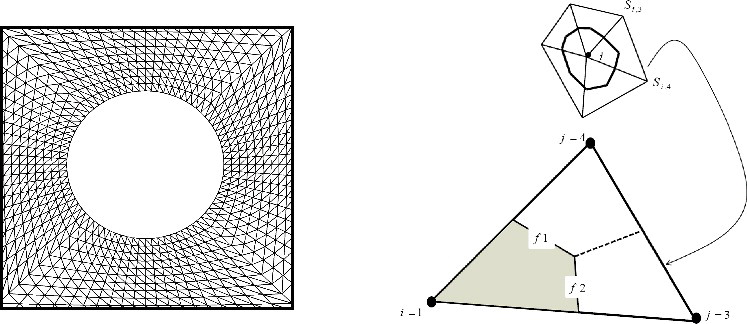
As seen in figure 3(a), triangular elements are considered as the building block of the discretization using CVFEM. The values of variables are approximated with linear interpolation within each element. A control volume is created by joining the centres of each element in the support to the midpoints of the element sides that pass through the central node i, which creates a close polygonal control volume (see figure 3(b)).

Figure 3. (a) Triangular elements around the pipeline, and (b) a sample triangular element and its corresponding control volume.

To illustrate the solution procedure using the CVFEM, one can consider the general form of advection–diffusion equation for node i in the following integral form: (17) or point form: (18) which can be represented by the system of CVFEM discrete equations as follows: (19)

In the above equation, the a's are the coefficients, the index (i, j) indicates the jth node in the support of node i, the index S_i,j provides the node number of the jth node in the support, the B's account for boundary conditions, and the Q's for source terms. For the selected triangular element which is shown in figure 3(b), this approximation without considering the source terms leads to (20)

Using upwinding, the advective coefficients, identified with the superscripts ()^u, are given by (21)

Also, the diffusion coefficients, identified with the superscripts ()^k, are given by (22)

In equation (21)(21) , the volume flow across faces 1 and 2 in the direction of the outward normal is (23)

The value of diffusivity at the midpoint of face 1 is given by (24)

Also, the corresponding value at the midpoint of face 2 is given by (25)

The velocity components at the midpoint of face 1 are (26)

and on face 2 are (27)

These values can be used to update the ith support coefficients through the following equation: (28)

In equation (21)(21) , moving in the counterclockwise direction around node i, the signed distances are (29) The derivatives of the shape functions are (30) and the volume of the element is (31)

The algebraic equations obtained from the discretization procedure using CVFEM are solved by the Gauss–Seidel method. Boundary conditions for the present problem can be applied using and as follows: (32) (33) where is the prescribed value on the boundary. The volume source terms can be applied as follows: (34) or after linearizing, the source terms can be applied as follows: (35)

4. Results and discussion

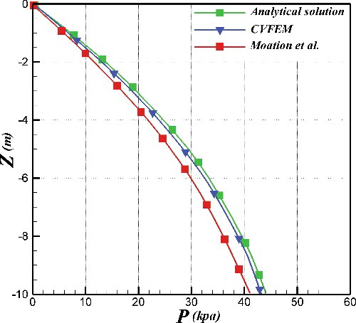
figure 4 shows the comparison between the results of Maotian et al. (2009), analytical results and the one obtained using CVFEM code. Maotian et al. used the FEM to solve their problem, and compared their results with an available analytical solution for a simple case. The comparison is carried out for , , . The thickness of homogeneous seabed is and the saturated unit weight and porosity of soil are and respectively. The submerged specific weight can be expressed as . The deformation modulus, Poisson's ratio and the permeability coefficient of soil are , and , respectively. As seen in this figure 4, the CVFEM is in better agreement with the analytical result compared to that of Maotian et al. (2009). CVFEM is a scheme that uses the advantages of both finite volume and finite element methods for simulation of multi-physics problems in complex geometries

Figure 4. Comparison of the present result with the analytical result and that obtained by Maotian et al. (2009).

The parameters used for numerical computations are the following: and The thickness of homogeneous seabed is and the unit weight and porosity of soil are and , respectively. The deformation modulus, Poisson's ratio and the permeability coefficient of soil are , and , respectively. The bulk modulus of pore fluid and unit weight of oil are and , respectively. The diameter, burial depth, unit weight and thickness of the pipeline are set to , , 21 and 0.2 m, respectively. The liquefaction potential is defined as , where is the initial mean effective stress of seabed and P is the accumulative pore pressure induced by seismic loading. The initial mean effective stress can be expressed as follows: (36) where is the coefficient of earth pressure at rest condition. In this study, when , liquefaction will occur.

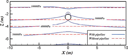
figure 5 shows the distribution of accumulative excess pore pressure in the vicinity of the pipeline. As seen in figure 5, the existence of pipeline has effect on accumulative excess pore pressure of seabed around the pipeline. At a given distance away from the pipeline, the effect of the existence of pipeline is slight and the distributions of both tend to be consistent. Variation of accumulative excess pore pressure is due to the change of shear and normal stresses around the pipeline. Moreover, the existence of the pipeline will change the draining path.

Figure 5. The distribution of accumulative excess pore pressure in the vicinity of the pipeline.

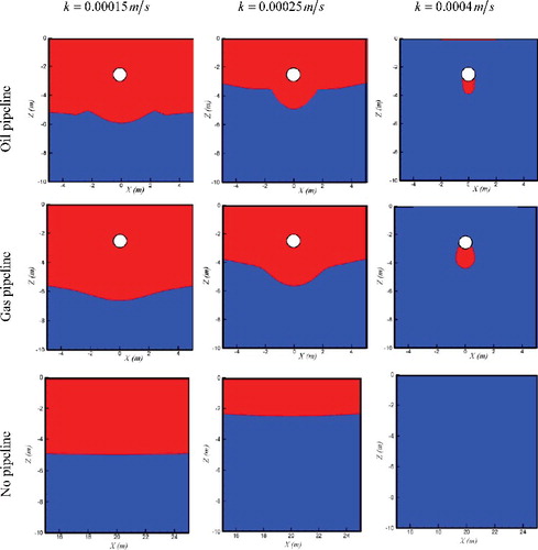
The effect of various permeability coefficients on liquefaction around the pipeline is shown in figure 6. The figure shows that with the growth of the liquefaction reduces noticeably. For the case of seabed with no pipeline, as enhances from to , the liquefaction area decreases, and afterwards, when increases up to , liquefaction would not occur. The liquefaction contours demonstrate that the existence of pipeline increases the liquefaction area, and at , liquefaction occurs around both the gas and oil pipelines. The figure also represents that at constant values of , the liquefaction area around the gas pipeline is much more than the oil pipeline. It is due to this fact that beneath the oil pipeline the effective stress is greater than that of the gas pipeline. The pipeline itself increases the liquefaction potential in the area around the pipeline. This increment is because the drainage path increases and also the density of fluid inside the pipeline is considerably less than the density of soil. The difference in density that led to the initial mean effective stress reduces.

Figure 6. The contour of liquefaction of soil for various values of around the gas pipeline, oil pipeline and for the seabed without pipeline. Liquefied area

, non-liquefied area

.

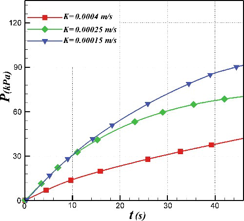
figure 7 shows the effect of permeability coefficients of soil on the time–history curve of accumulative excess pore pressure at the bottom of the pipeline when the other parameters are constant. It is observed that the accumulative excess pore pressure of seabed at the bottom of the pipeline is significantly affected by variable permeability. Accumulative excess pore pressure increases as the value of permeability coefficient decreases. Decreasing the soil permeability coefficient reduces the movement of pore water with respect to soil skeleton. The pore water displaces together with the soil skeleton. Since hardly any volume change is possible, due to the large stiffness of the pore water, the whole tendency of required volume change for the adjustment of soil particles, under applied load, causes a corresponding change in the pore-water pressure. In this case, deformation leads to an increase in pore pressure.

Figure 7. Development of accumulative excess pore pressure at the bottom of the pipeline with various deformation moduli of soil.

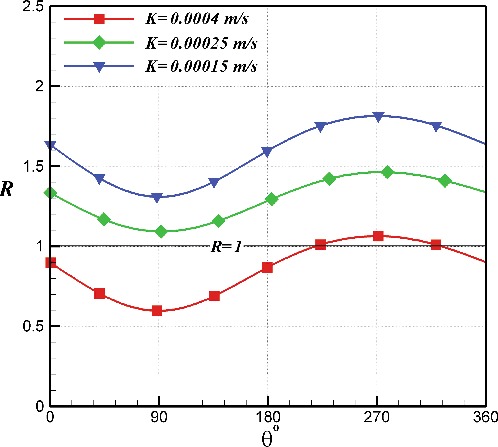
figure 8 shows the distribution of liquefaction potential around the pipeline with permeability coefficients of soil. As seen, the maximum and minimum values of liquefaction potential occur at the bottom and top of the pipeline, respectively. This behaviour can be explained with the fact that in seabed, the drainage path for the top of the pipeline is shorter than the bottom of the pipeline, and dissipation of pore-water pressure occurs faster. In addition, the figure indicates that the increase of the permeability coefficient causes the values of R to decrease. For example, the values of liquefaction potentials around the pipeline are more than 1.0 when the permeability coefficient of soil is . It implies that liquefaction occurs in all regions around the pipeline under this condition. When , liquefaction occurs at around the pipeline. However, liquefaction does not occur at any part of the seabed around the pipeline under this condition.

Figure 8. Distribution of liquefaction potential around the pipeline with permeability coefficients of soil.

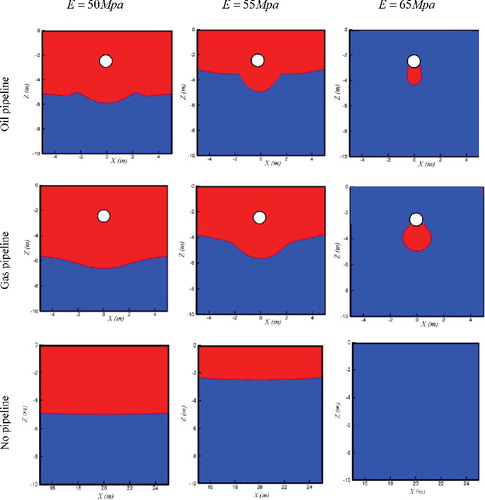
The deformation modulus of soil increases significantly with the increase of soil density. In practical works, the sediment is sometimes compacted to desired deformation modulus. figure 9 shows the effect of different deformation moduli on the extension of the liquefaction area around the pipeline, and in this case, there is no pipe inside the seabed. As seen, with the increase of , the liquefaction reduces. For the seabed without pipeline with the growth of E from to , the liquefaction area diminishes noticeably; afterwards, when E increases up to , the liquefaction phenomena will not be occurred. The liquefaction contours indicate that the existence of pipeline augments the liquefaction area, and at , liquefaction is occurred around both the gas and oil pipelines.

Figure 9. The contour of liquefication of soil for various values of around the gas pipeline, oil pipeline and for the seabed without pipeline Liquefied area

, non-liquefied area

.

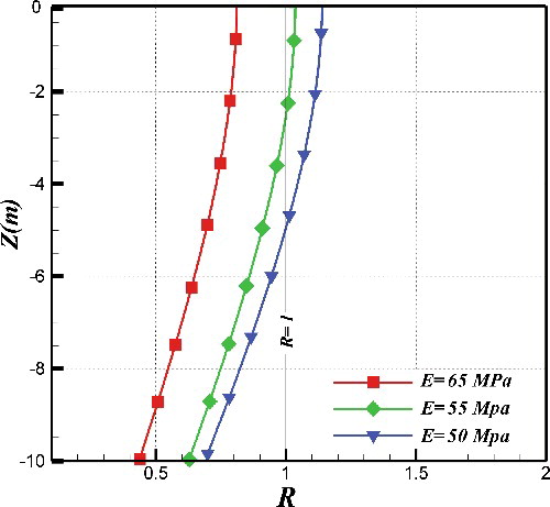
figure 10 shows the vertical distribution of liquefaction potential along the centreline of the seabed with various deformation moduli of soil for the case of seabed without pipeline. As can be seen, liquefaction potential of the seabed decreases with the depth increasing, because the rate of increasing effective stress becomes greater than the rate of increase in accumulative excess pore pressure. The figure also indicates that at the same depth, the liquefaction potential of the seabed increases with the deformation modulus of soil decreasing. This behaviour can be explained with the fact that the higher the stiffness, the smaller the strain induced by the same earthquake loading; therefore, lower accumulative excess pore pressure can be generated. When the deformation modulus of the soil is 50 MPa, it shows that liquefaction occurs within the depth of seabed z = 4.6 m. When the deformation modulus of the soil is 55 MPa, the liquefaction potential occurs within the depth of seabed z = 2.3 m. The liquefaction potential at any depth of seabed are all <1, when the deformation modulus of soil is 65 MPa, and it indicates that liquefaction does not occur at any depth under this condition.

Figure 10. Vertical distribution of liquefaction potential along the centreline of the seabed with various deformation moduli of soil.

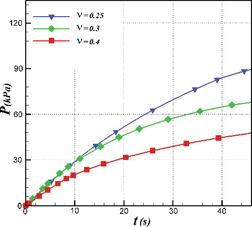
figure 11 presents the effect of Poisson's ratio of soil on the time–history curve of accumulative excess pore-water pressure at the bottom of the pipeline when the other parameters are constant. Similar to the increase of E and k, the increase in the Poisson's ratio of soil causes the values of accumulative excess pore to reduce. This behaviour may be attributed to the fact that the volume change potential decreases when the values of Poisson's ratio of soil increases. For undrained seismic deformation, the soil behaviour is governed by the interaction between the soil particles and pore water. In the case of a constant volume, undrained deformation causes no change in the pore-water pressure.

Figure 11. Development of accumulative excess pore pressure at the bottom of the pipeline with various Poisson's ratios of soil.

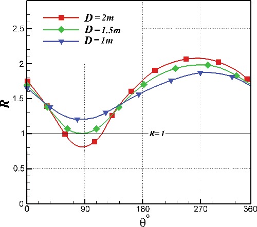
figure 12 shows the distribution of liquefaction potential around the pipeline with various diameters of the pipeline. The figure shows that increasing the diameter of pipeline increases the liquefaction potential in some area, while it decreases the potential in the other parts. This is due to the change of accumulative excess pore pressure and initial mean effective stress of seabed around the pipeline. The change in accumulative pore-water pressure occurs as the result of change in the distance of points around the pipeline from the seabed surface (accumulative excess pore-water pressure = 0); the more distance the more accumulative excess pore-water pressure. The increase of pipeline diameter also leads to the increase of draining path under pipeline between 180° and 360° due to the impermeability of the pipeline. Moreover, distribution of mean effective stress of soil around the pipeline wall changes with the diameter of pipeline. Increasing diameter of pipeline increases the z-coordinate of soil in the regions of 180° < θ < 360°, but reduces the z-coordinate of soil at 0° < θ < 180°. Therefore, the initial mean effective stress and accumulative excess pore pressure of soil around the pipeline change with the diameter of pipeline. When the rate of increasing accumulative excess pore pressure exceeds the rate of increasing initial mean effective stress, the accumulative excess pore-pressure ratio increases, otherwise it reduces.

Figure 12. Distribution of liquefaction potential around the pipeline with various diameters of the pipeline.

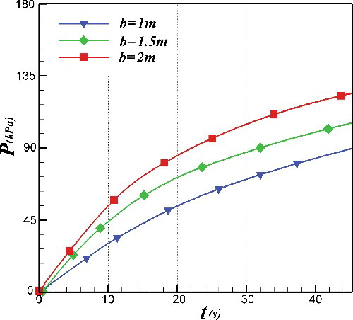
figure 13 shows the time–history curves of seismic accumulative excess pore pressure at the bottom of the pipeline with various burial depths of the pipeline. As seen in figure with the pipeline burial depth increasing, the seismic accumulative excess pore pressure increases. This increment can be explained by the fact that by increase of burial depth the distance between the bottom of the pipeline from the seabed surface increases. Therefore, the drainage path increases and during the short duration of earthquake, the accumulative excess pore-water pressure cannot be dissipated.

Figure 13. Development of accumulative excess pore pressure at the bottom of the pipeline with various burial depths of the pipeline.

5. Conclusion

The CVFEM is used to investigate the effect of different physical and geometrical parameters on liquefaction around a pipeline inside porous seabed. From this investigation, some conclusions were summarized as follows:

1. Comparison of the present result with the previous analytical and numerical works revealed the accuracy and applicability of the CVFEM in geotechnical investigations.

2. The most critical point in terms of liquefaction potential is the bottom of the pipeline.

3. With the increase of deformation module (), Poisson's ratio () and permeability of the soil coefficient (), the liquefaction potential reduces.

4. Increase of pipeline diameter causes an increase in liquefaction potential in some areas around the pipeline. In addition, the pore-water pressure around the pipeline increases with the increase of the burial depth.

5. The liquefaction potential around the gas pipeline is slightly more than the oil pipeline at constant parameters.

Disclosure statement

No potential conflict of interest was reported by the authors.

Appendix. List of symbols

Table

	Pore pressure
	Unit weight of pore water
	Unit weight of oil
	Permeability coefficient of soil
	Deformation modulus
	Bulk modulus of pore fluid
	Poisson's ratio of soil
	Accumulative excess pore pressure source term
	Period of equivalent cyclic stress
	Duration of earthquake
	Initial mean effective stress
	Unit weight of soil
	Submerged specific weight of soil
	Depth of calculation point to the surface
	Gravitational acceleration
	Maximum ground acceleration
	Reduction coefficient of stress
	Porosity of soil
	Diameter of pipeline
	Coefficient of earth pressure at rest condition
	Width of the computation region
and	Centre coordinates of pipeline
	Two-dimensional consolidation coefficient
	Volume of the element
	Thickness of homogeneous seabed
	Value on the boundary
	Width of the computation region
	Burial depth of the pipeline
	Liquefaction potential

References

- Alba PD, Seed HB, Chan CK. 1976. Sand liquefaction in large-scale simple shear tests. J Geotech Eng Div. 102:909–927.
- Azadi M, Hosseini MM. 2010a. Analyses of the effect of seismic behavior of shallow tunnels in liquefiable grounds. Tunn Undergr Space Technol. 25:543–552.
- Azadi M, Hosseini MM. 2010b. The uplifting behavior of shallow tunnels within the liquefiable soils under cyclic loadings. Tunn Undergr Space Technol. 25:158–167.
- Biot MA. 1941. General theory of three-dimensional consolidation. J Appl Phys. 12:155–164.
- Bobe A. 2003. Effect of pore water pressure on tunnel support during static and seismic loading. Tunn Undergr Space Technol. 18:377–393.
- Bransby MF. Newson TA. Brunning P. 2002. The upheaval capacity of pipelines in jetted clay backfill. Int J Offshore Polar Eng. 12:280–287.
- Chen CH, Wang TT, Jeng FS, Huang TH. 2012. Mechanisms causing seismic damage of tunnels at different depths. Tunn Undergr Space Technol. 28:31–40.
- Cheuk CY, Take WA, Bolton MD, Oliveira JRMS. 2007. Soil restraint on buckling oil and gas pipelines buried in lumpy clay fill. Eng Struct. 29:973–982.
- Choobbasti AJ, Tavakoli H, Kutanaei SS. 2014. Modeling and optimization of a trench layer location around a pipeline using artificial neural networks and particle swarm optimization algorithm. Tunn Undergr Space Technol. 40:192–202.
- Chou HS, Yang CY, Hsieh BJ, Chang SS. 2001. A study of liquefaction related damages on shield tunnels. Tunn Undergr Space Technol. 16:185–193.
- Hashash YMA, Hook JJ, Schmidt B, Yao JI. 2001. Seismic design and analysis of underground structures. Tunn Undergr Space Technol. 16:247–293.
- Janalizadeh A, Kutanaei SS, Ghasemi E. 2013. Control volume finite element modeling of free convection inside an inclined porous enclosure with a sinusoidal hot wall. Sci Iran. 20:1401–1414.
- Jeng DS, Zhang H. 2005. An integrated three-dimensional model for wave- induced pore pressure and effective stresses in a porous seabed. II: breaking waves. Ocean Eng. 32:1950–1967.
- Kirca VO, Sumer BM, Fredsøe J. 2014. Influence of clay content on wave-induced liquefaction. J Waterway Port Coastal Ocean Eng. 140:04014024.
- Kouretzis GP, Bouckovalas GD, Karamitros DK. 2011. Seismic verification of long cylindrical underground structures considering Rayleigh wave effects. Tunn Undergr Space Technol. 26:789–794.
- Kutanaei SS, Choobbasti AJ. 2015a. Prediction of combined effects of fibers and cement on the mechanical properties of sand using particle swarm optimization algorithm. J Adhes Sci Technol. 29:487–501.
- Kutanaei SS, Choobbasti AJ. 2015b. Mesh-free modeling of liquefaction around a pipeline under the influence of trench layer. Acta Geotech. 10:343–355.
- Kutanaei SS, Ghasemi E, Bayat M. 2011. Mesh-free modeling of two-dimensional heat conduction between eccentric circular cylinders. Int J Phys Sci. 6:4044–4052.
- Kutanaei SS, Roshan N, Vosoughi A, Saghafi S, Barar B, Soleimani S. 2012. Numerical solution of stokes flow in a circular cavity using mesh-free local RBFDQ. Eng Anal Boundary Elem. 36: 633–638.
- Liao S, Whitman R. 1986. Overburden correction factors for SPT in sand. J Geotech Eng. 112: 373–377
- Liu H, Jeng DS. 2007. A semi-analytical solution for random wave-induced soil response and seabed liquefaction in marine sediments. Ocean Eng. 34:1211–1224.
- Maotian L, Xiaoling Z, Qing Y, Ying G. 2009. Numerical analysis of liquefaction of porous seabed around pipeline fixed in space under seismic loading. Soil Dyn Earthq Eng. 29:855–864.
- Rezaei S, Choobbasti AJ, Kutanaei SS. 2015. Site effect assessment using microtremor measurement, equivalent linear method, and artificial neural network (case study: Babol, Iran). Arab J Geosci. 8:1453–1466.
- Sarokolayi LK, Beitollahi A, Abdollahzadeh G, Amreie ST, Kutanaei SS. 2015. Modeling of ground motion rotational components for near-fault and far-fault earthquake according to soil type. Arab J Geosci. 8:3785–3797.
- Sedarat H, Kozak A, Hashash YMA, Shamsabadi A, Krimotat A. 2009. Contact interface in seismic analysis of circular tunnels. Tunn Undergr Space Technol. 24:482–490.
- Seed HB, Martin PP, Lysmer J. 1976. Pore-water pressure changes during soil liquefaction. J Geotechnol Eng Div. 102:323–346.
- Seed HB, Rahman MS. 1978. Wave-induced pore pressure in relation to ocean floor stability of cohesionless soils. Mar Geotechnol. 3:123–150.
- Sheikholeslami M, Gorji-Bandpy M, Ganji DD, Soleimani S. 2013. Effect of a magnetic field on natural convection in an inclined half-annulus enclosure filled with Cu-water nanofluid using CVFEM. Adv Powder Technol. 24:980–991.
- Sheikholeslami M, Gorji-Bandpy M, Ganji DD, Soleimani S. 2014. Heat flux boundary condition for nanofluid filled enclosure in presence of magnetic field. J Mol Liq. 193:174–184.
- Sheikholeslami M, Gorji-Bandpy M, Ganji DD, Soleimani S, Seyyedi SM. 2012. Natural convection of nanofluids in an enclosure between a circular and a sinusoidal cylinder in the presence of magnetic field. Int Commun Heat Mass Transf. 39:1435–1443
- Soleimani S, Ganji DD, Gorji M, Bararnia H, Ghasemi E. 2011. Optimal location of a pair heat source-sink in an enclosed square cavity with natural convection through PSO algorithm. Int Commun Heat Mass Transf. 38:652–658.
- Soleimani S, Jalaal M, Bararniaa H, Ghasemi E, Ganji DD, Mohammadi F. 2010. Local RBF-DQ method for two-dimensional transient heat conduction problems. Int Commun Heat Mass Transf. 37:1411–1418.
- Soleimani S, Sheikholeslami M, Ganji DD, Gorji-Bandpay M. 2012 Natural convection heat transfer in a nanofluid filled semi-annulus enclosure. Int Commun Heat Mass Transf. 4:565–574.
- Sumer BM. 2014. Liquefaction around marine structures. London: World Scientific.
- Sumer BM, Fredsøe J. 2002. The mechanics of scour in the marine environment. London: World Scientific.
- Sumer BM, Kirca VSO, Fredsøe J. 2012. Experimental validation of a mathematical model for seabed liquefaction under waves. Int J Offshore Polar Eng. 22:133–141.
- Sumer BM, Truelsen C, Fredsøe J. 2006. Liquefaction around pipelines under waves. J Waterway Port Coastal Ocean Eng. 132:266–275.
- Tavakoli HR, Kutanaei SS. 2015. Evaluation of effect of soil characteristics on the seismic amplification factor using the neural network and reliability concept. Arab J Geosci. 8:3881–3891.
- Unutmaz B. 2014. 3D liquefaction assessment of soils surrounding circular tunnels. Tunn Undergr Space Technol. 40:85–94.
- Wang WL, Wang TT, Su JJ, Lin CH, Seng CR, Huang TH. 2001. Assessment of damages in mountain tunnels due to the Taiwan Chi-Chi earthquake. Tunn Undergr Space Technol. 16:133–150.
- Winslow AM. 1966. Numerical solution of the quasilinear Poisson equation in a nonuniform triangular mesh. J Comp Phys. 1:149–172.