Crustal imaging of the Northwest Himalaya and its foredeep region from teleseismic events

ABSTRACT

Over 450 receiver functions from 8 broadband stations located in the Indo-Gangetic plain and Northwest Himalayan region are analyzed to examine the crustal properties across the contiguous region. We identified the P-to-S phase beneath each station and estimated the crustal thickness from time delay of this phase with respect to the direct P arrival. With the help of the slant stacking technique, we determined bulk crustal chemical properties and validated our estimate of crustal thickness. The Moho was encountered in the Indo-Gangetic plain at an average depth of 33 km and thickened towards the Northwest Himalaya with the Moho depth varying from 37 to 52 km. The thickest crust matched the highest topography, which is strong evidence of the occurrence of a crustal root of the mountain range. The time domain iterative linearized inversion technique is used to invert radial receiver functions to wave velocity structures for both tectonic regimes. From the forward modelling, we found mid-crustal low-velocity layers at different patches at a depth of 10–30 km in the Northwest Himalaya region. The presence of melts may be inferred in the mid crust with high values of Poisson ratio (σ ≥ 0.260) for the stations in the Northwest Himalaya. Towards south in the Indo-Gangetic alluvium plain, we estimated a medium to higher value of Poisson ratio (0.240 ≤ σ ≤ 0.290), but velocity modelling implies absence of an intracrustal low-velocity zone around the region.

KEYWORDS:

• Northwest Himalaya
• Indo-Gangetic basin
• receiver function
• 1-D velocity model
• Vp/Vs ratio

1. Introduction

The Himalayas were formed due to the collision of the Indian continent with the Eurasian continent (Wadia 1931; Molnar et al. 1973; Molnar & Tapponiar 1975; Ni & Barazangi 1984) 50 Ma, becoming the world's longest mountain range. The Himalayas occupy the northern part of the Indian continent, forming an arc of about 400 km width bending convex to south–south-west. This arc is unbroken for 2400 km, running along the mountain ranges of Hindu Kush and Pamir on its western margin to the Arunachal Himalayas on its easternmost margin. The northern part may be regarded more or less as a continuous depression running parallel to the Himalayan arc and comprising the valleys from where the large rivers the Indus and the Tsangpo originate.

The present-day deformation is due to the continental–continental collision of the Indian plate under thrusting beneath the Eurasian plate at a rate of 10–20 mm/yr (Jade 2004). With the collision process that started 55 Ma (Besse & Courtillot 1988), the Indian plate moves towards north-east at a convergence rate of 55 mm/yr, of which 18–20 mm/yr is consumed under the Himalayas (Bilham & Gaur 2000; Jade 2004). The accumulated strain energy is being released in the form of large and major earthquakes. In the last two decades, this region has experienced many devastating earthquakes such as the great Kangra earthquake (Mw 8.0, 1905), Uttarkashi earthquake (Mw 6.8, 20 October, 1991) and Chamoli earthquake (Mw 6.4, 29 March, 1999), Kashmir earthquake (Mw 7.6, 2005, Kayal 2007), Kunlun earthquake (Mw 8.1, 2001; Fu & Lin 2003) and Wenchuan earthquake (M 8.0, 2008; Zhang et al. 2009). These earthquakes have enhanced the consciousness about the increasing disaster and vulnerability of this highly populated region. It has also been argued that an impending large earthquake of Mw ∼ 8.8 is expected in the region (Bilham & England 2001), which may cause a greater destruction to the northern part of the Indian territory.

Over the last two decades, many earth scientists have tried to map the lithospheric image of the Northwest Himalaya. Rai et al. (2006) studied the teleseismic receiver function in the Ladakh and Northwest Himalaya, along a 700-km-long profile across the Main Central Thrust (MCT), Main Boundary Thrust (MBT) and the Himalayan Frontier Thrust (HFT) from the Indo-Gangetic basin to the Karakoram fault. They have found out that the Moho depth reached up to 75 km on Ladakh–Karakoram and the thickness of Moho decreased southward to 40 km near the Indo-Gangetic basin. Caldwell et al. (2009) reported a mid-crustal channelized liquid flow or a low-velocity layer (LVL) from the southern Tibet detachment to the Northwest Himalaya region, in agreement with the previous magnetotelluric (MT) study by Gokarn et al. (2002) and Arora et al. (2007). The MT study by Arora et al. (2007) inferred the presence of a low-resistivity (5–10Ω) layer in the middle crust from the southern detachment to Karakoram fault (KF). Gokarn et al. (2002) and Harinarayana et al. (2004) inferred from their studies that the presence of a low-resistivity layer can be attributed to partial melts, aqueous fluid or graphite in the region. Although MT data cannot distinguish between the magmatic flow and aqueous flow, but it points to the fact that there is a large viscosity drop in the Northwest Himalaya. Kumar et al. (2009) determined a 1-D velocity model by travel time inversion and inferred that the Moho depth in the Northwest Himalaya region lies at an average depth of 44 km with some mid-crustal fluid filled detachment plane stretching from 15 km to 18 km. Recently, Srinagesh et al. (2011) suggested the presence of an aqueous medium flowing in the middle crust, which goes down to the mantle in the higher Himalaya through the entire Northwest Himalayan up to KF.

In the receiver function technique, the teleseismic body waveforms are used to image the crustal structures underneath the seismic stations (Chevrot & Van Der Hilst 2000). The arrival time of the Ps, PpPs and PpSs + PsPs converted and reverberated phases from the Moho can be combined to constrain the mean crustal thickness and Vp/Vs ratio (Zhu & Kanamori 2000). To model the Earth velocity structure using these converted phases at the receiver, it is necessary to separate these phases from the effect of source, path and instrument, which govern the shape of the waveform. The teleseismic waveform contains information about the source, site characteristics and propagation path effect through the mantle and local sites underneath the seismic station. The deconvolution of the vertical component from the radial and tangential component seismograms removes information common to both and leaving a time series, showing the site response or “receiver function” (Ammon et al. 1990; Gurrella et al. 1995).

In this study, we use the receiver function methodology to map the crustal structure of the Northwest Himalaya and the Indo-Gangetic basin through the inversion of teleseismic body waveforms. Moreover, we also tried to decipher the similarities and dissimilarities between the two different tectonic regimes in terms of Moho depth, Vp/Vs and Poisson ratio.

2. Tectonic setup

The Himalayan mountain system comprises various tectonic belts such as the Trans Himalaya belt or the main central crystalline belt, which is also called the Greater or higher Himalaya having an average elevation of 7300 m. The lesser Himalaya comprises mostly mountains with an elevation of up to 4500 m and the southern outer territory foothills with an average elevation of 1300 m. The boundaries between various belts are marked by major thrusts and faults that can be traced semi-continuously for long distances (figure 1). From the seismotectonic point of view, the evolution, structure and tectonic activity of the Himalaya depend largely on the major tectonic features such as the Indus–Tsangpo suture zone (ISZ), MCT, MBT and HFT and their behaviour at different depths (Yin 2006). Some of these faults are very prominent and visible at the surface but some faults are hidden (figure 2). The HFT is the southernmost, younger and neo-tectonically active thrust of the Himalayan region, giving a topographical break to the Himalayas, against the alluvial Indo-Gangetic plain. The Indo-Gangetic plain was formed as a consequence of the lithospheric flexing due to the continued push of the Indian plate towards the Himalayan orogeny (Srinagesh et al. 2011). The complex geological tectonics of the Indo-Gangetic plain comprises many ridges, lineaments, and thick alluvial sedimentation by the Indus, Ganges and other rivers.

Figure 1. Geological map of North India and Himalayan Mountain range (following Guillot et al., 2008). Box area in the picture represented the study region of the present study.

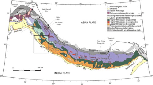
Figure 2. The above tectonic map of northwestern Himalaya with major fault system, terranes and suture zones including MBT (Main Boundary Thrust), MCT (Main Central thrust), HFT (Himalayan Frontier Thrust), STD (Southern Tibetan detachment) and KF (Karakoram Fault). Distribution of the seismic stations of IMD network stations are denoted by filled black triangles along with seismicity observed in fifty years with earthquakes of magnitude 3 and above.

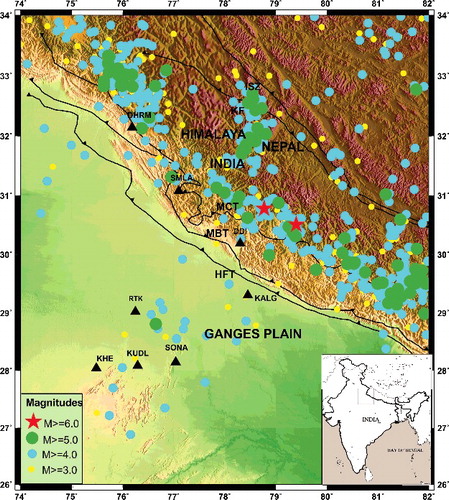
The thrust faults in the Himalayan region are capable of producing great earthquakes. Some of these are very prominent and visible at the surface but some faults are hidden. These faults are associated with a number of small transverse folds, faults and fractures throughout the mountain system. Most of the seismicity is concentrated in the lesser Himalayas within a 50-km-wide zone between the MBT and MCT. This zone is referred to as the Main Himalayan seismic belt (Ni & Barazangi 1984). Most of these moderate earthquakes occur at shallow depths (10–20 km) within the crustal section of the Northwest Himalaya (Seeber et al. 1981; Ni & Barazangi 1984). Along with it, the southern frame of the Himalayas comprises many hidden ridges and faults located beneath the Ganges basin. This complex setting is well defined by the geodetic movements, geological features and seismic gaps or by analyzing spatial and temporal patterns of seismicity (figure 2) (Pandey et al. 1995; Kayal 2001; Bollinger et al. 2004; Gitis et al. 2008; Kumar et al. 2009).

3. Data and methodology

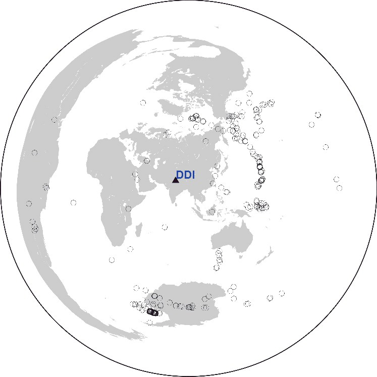
We have used teleseismic earthquakes recorded by eight permanent stations established by Indian Meteorological Department (IMD) in the Northwest Himalaya and Indo-Gangetic plain. Relatively good quality seismic data is collected from these eight broadband seismic stations situated in the Northwest Himalaya and its foredeep region. The teleseismic waveforms of magnitudes mb ≥5.5 and high signal-tonoise ratio (SNR >2.5) are selected for this present study. We considered teleseismic waveforms with an epicentral distance varying between 30° and 90° to avoid wave field complexities of upper mantle discontinuities or diffraction at the core–mantle boundary. A total of 110 earthquakes, mostly from the Circum Pacific belt (figure 3), were used to produce 479 individual receiver functions for all those eight broadband stations. The range of band pass period best suited for our analysis is 1.5–12 sec such that the resultant filtered RF comes out with stronger peaks of Ps and its multiples.

Figure 3. Distribution of teleseismic earthquakes used for P receiver function analysis in this study.

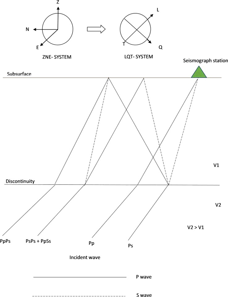
The P wave receiver function analysis has now become a conventional method to determine the crust and upper mantle structures beneath a seismic station. It eliminates the influence of source, path and instrumental response. The RF mainly contains converted Ps and multiple reflection (PpPs, PpSs + PsPs, etc) phases (figure 4) generated at the crust and upper mantle discontinuities below the seismic stations (Vinnik 1977; Ammon et al. 1990). The receiver function technique has been widely used all over the world to study the interior structure of the Earth since they were introduced four decades ago (Langston 1977). Primarily the RF was mainly used to investigate the crustal structure beneath the seismic station (Owens et al. 1984; Ammon 1991). More advanced receiver function stacking methods have been developed recently to study the crust and upper mantle discontinuities of the complex tectonic region. To determine the RF, three-component (ZNE) seismograms are rotated first to the LQT (or P-SV-SH) coordinate system, where L is the direction of incident P wave, and Q is perpendicular to the L component and points away from the source, and T is the third direction in the right-handed coordinate system (Kind et al. 1995; Yuan et al. 1997). P wave energy is mainly concentrated in L, while Q and T components have SV and SH wave energies, respectively. Receiver functions are obtained by deconvolving P waveforms on the L component from the corresponding Q component and T component, respectively. A time domain deconvolution procedure is used. First, we generate an inverse filter in the time domain by minimizing the least-squares difference between the L component and the desired delta-like spike function of normalized amplitude. Spiking deconvolution in time domain on the Q component enhances the converted phases of receiver functions, while the T component indicates the lateral variation or anisotropic medium underlying the geology.

Figure 4. A schematic diagram representing receiver functions simplified ray trace diagram presenting main P-to-S converted phases and many reverberations for a horizontal layer over a half space. For the phase representation upper case letters denote downgoing travel paths, lowercase letters denotes upgoing travel paths. The LQT system represents the corresponding wavefield components after doing rotation from ZNE components.

Receiver functions can be inverted for shear velocity structure beneath a given seismic station by minimizing the difference between the observed and synthetic receiver functions (Ozalaybey et al. 1997; Liggoria & Ammon 1999). Before the inversion process, we resampled the data into 10 samples/sec, chose a time interval 5 sec before and 25 sec after the direct P arrival, used tapering at the ends of the cut seismogram, and finally constructed a receiver function using a Gaussian width 2.5 and water level parameter 0.001. Finally, we stacked receiver functions to enhance the SNR.

We employed the H-k stacking of Zhu and Kanamori (2000) for simultaneous determination of the Moho depth and Vp/Vs (k) ratio. Assuming the crust is homogeneous with Moho depth ‘H’, the delay time of the Moho Ps phase and other multiples can be expressed as (Yuan et al. 2001) (A1) (A2) (A3) where p is the ray parameter defining the slowness of the medium.

Thus, the delay times depend on three crustal parameters: H, Vp and Vs. Since they are more sensitive to the Vp/Vs ratio ‘k’ than to Vp, we fixed Vp as a known parameter. Then, the delay times () depend only on ‘H’ and Vs.

The ratio Vp/Vs can be calculated as (A4) Here

The arrivals of the maximum amplitude of the Moho Ps and PpPs pulse were picked on the stacked receiver functions at each station after the moveout correction for the corresponding phase. The reference epicentre used for moveout correction is 67° and the corresponding ray parameter is 6.4 s/° (Yuan et al. 2000). As the Moho depth and Vp/Vs are not sensitive to the variation of the P-wave velocity, it is possible to estimate both the average Moho depth and Vp/Vs (simply ‘k’), assuming crustal Vp as 6.4 km/s. The grid search method by Zhu and Kanamori (2000) estimates both the Moho depth and the Vp/Vs ratio with a high confidence that can be defined by the H–k domain in a space s as (A5) where r(t) is the radial receiver function, weighting factors with Σw_i = 1. The stacking receiver functions from events at different distances reach a maximum when all the three phases are stacked coherently to estimate of H and k. where σ_s is the estimated variance of s (H,k) from stacking. We can estimate Poisson's ratio (σ) from the Vp/Vs ratio using the relation (A6)

In this study, the receiver functions at each station were stacked by using equation (A5)(A5) with w₁ = 0.5, w₂ = 0.3 and w₃ = 0.1, respectively. These values were chosen to balance the weights for the Moho Ps phase and its later multiple phases. We also tried different weights (w₁ = 0.7, w₁ = 0.3, w₁ = 0.1) to perform H–k stacking, and found that the weights w₁ = 0.5, w₂ = 0.3 and w₃ = 0.1 provide best results. The arrival times of various converted multiple phases, crustal thickness, Vp/Vs and Poisson ratio is shown in table 1.

Table 1. Station Locations with their tectonic block, number of receiver functions, the average Vp, along with quality of Z-K figure used to derive the crustal parameters.

STN.	LAT (°N)	LONG (°E)	ELV. (meter)	TECT. BLOCK	No. RFs	Ps (sec)	PpPs (sec)	PsSs (sec)	Vp/Vs	H (KM)	Mean PR (σ)	Quality
DHRM	32.15	76.19	1995	NW Himalaya	86	5.9	11.0	16.1	1.801 ± 0.03	52 ± 2	0.277	A
SMLA	31.07	77.10	2200	NW Himalaya	85	5.3	10.5	14.0	1.760 ± 0.08	37.5 ± 2	0.262	A
DDI	30.19	78.30	682	NW Himalaya	105	5.2	12.0	16.0	1.890 ± 0.05	42 ± 2	0.308	A
KALG	29.30	78.45	1814	NW Himalaya	76	4.8	10.0	14.5	1.740 ± 0.06	35.8 ± 2	0.253	A
KUDL	28.08	76.29	227	Indian Shield	29	4.5	10.0	17.0	1.835 ± 0.04	34 ± 2	0.287	A
KHE	28.14	77.03	180	Indian Shield	52	4.2	10.0	13.0	1.800 ± 0.07	32.5 ± 2	0.277	B
SONA	28.04	75.48	320	Indian Shield	21	4.1	10.5	15.5	1.785 ± 0.10	34 ± 2	0.269	A
RTK	29.02	78.25	300	Indian Shield	45	4.0	11.0	14.5	1.850 ± 0.05	31 ± 2	0.330	C

STN.: Station name, LAT: latitude, LONG: longitude, TECT. BLOCK: Tectonic Block, RFs: Receiver Functions, H: Depth, PR: Poisson Ratio

4. Results

4.1. Moho depths beneath the Northwest Himalaya and Indo-Gangetic basin

4.1.1. Northwest Himalaya

All the receiver functions are plotted with respect to the direct P wave arrival, and most of the energy in the RFs after the direct P phase is due to the Moho converted P-to-S phase and its multiples. The RFs of all eight stations are plotted with respect to back azimuths (figure 5). Some strong peaks of converted phases are also observed just after the direct P arrival, indicating the presence of significant intra-crustal discontinuity. In order to enhance the amplitudes of different phases, all RFs were filtered by a low pass 2 sec and a high pass 10/12 sec prior to stacking. Stacking of the events with a narrow back azimuth bin can produce broader peaks for Moho converted Ps and multiple phases because of the dependence of the arrival time on back azimuth. We stack receiver functions at each station according to earthquake backazimuth. The stacks binned in 10° azimuth interval are used for most of stations for good amount of quality data. It has been observed that some of the stations do not have good backazimuth coverage. For these stations, the bin is increased to 30°. At most stations, the receiver function (RF) exhibits strong P-to-S conversions from the Moho and crustal discontinuities are identified on different azimuth stacked RF traces.

Figure 5. Receiver function traces derived by stacking at different azimuth (stacked by 10° bin for DDI, DHRM, SMLA, SONA, KUDL and RTK and stacked by 30° bin) for the stations located at Northwest Himalaya and Indian shield region. On the top panel, the summation trace for each station, the Moho P-to-S converted phase and its multiple phases are donated by 1 (Moho Ps), 2(PpPs) and 3 (PsPs+PpSs) inside the inverted pentagon.

The station DDI (32.15°N; 76.19°E) is located in the Northwest Himalaya in between HFT and MCT. Visual inspection of the radial (here QRF) receiver functions at DDI indicates an early arrival at about 2.0 sec, which can be associated with a converted P-to-S wave from a shallow interface of 13–15 km. The Ps arrival at about 5.2 sec seems to be generated at the Moho interface. In the upper crust, our analysis shows some negative phase around ∼2–3 sec. Caldwell et al. (2013) and Kumar et al. (2009) had reported LVZ at a depthbelow 15 km in this region. The stacked RF shows prominent positive arrivals at ∼5.2 sec and ∼12.0 sec and a negative phase arrival at ∼16.0 sec. These phases can be identified as Moho converted Ps, PpPs and PpSs+PsPs arrivals, respectively (table 1). In the DDI station we see a time lag on the Ps-phase arrival 90°–120° backazimuth, which may signify the Moho is dipping towards north of lower to higher Himalaya. The station DHRM (32.15°E, 76.19°N) situated on the MBT has one of the best data quality set we have in our analysis. There is a strong crustal P-to-S conversion (figure 5) at 5.9 sec, which corresponds to a thicker crust. The result agrees with Caldwell et al. (2013) and Srinagesh et al. (2011) as they reported a Moho depth of nearly 50 km near the station DHRM. The negative phase arrival at ∼3.0 sec can be attributed to the presence of a mid-crustal low-velocity layer beneath the station. The stacked RFs at all backazimuth show a PpPs phase at around 10.5 sec and a faint PpSs+PsPs arrival at 16.1 sec. Similar to the DDI station, the Moho Ps conversion shows some delay in different backazimuth arrival events from 30° to 130°, representing laterally dipping or anisotropic structure. The station SMLA located in between MBT and MCT is characterized by a complex receiver function with a first large positive conversion arriving nearly at 3.5 sec after the direct P. The later converted phase at 5.3 sec may be from the Moho and is consistent with the previous MT studies in the region (Arora et al. 2007), which provides a Moho depth of around 40 km. The strong positive amplitude peak arrived at 10.5 sec represents the PpPs phase, while the negative amplitude PpSs+PsPs phase arrives at nearly 14.0 sec. The station KALG (29.30°E, 78.45°) is situated just beneath MBT located on the foothills of the lower Himalaya. There is no azimuthal variation observed in the RF data of KALG station. After the direct P phase we get a negative pulse at 2–3 sec. The strong amplitude peaks on every backazimuth at about 4.8 sec are considered as the Ps phase converted from the Moho. The other multiples (PpPs, PpSs + PsPs) are weak due to similar amplitude coherent phases that reverberated from some other discontinuity. Along with the converted Moho Ps phase at around 4.8 sec, weak amplitudes of the PpPs phase are observed at around 10.0 sec and the PpSs+PsPs phase observed at around 14.5 sec.

4.1.2. Indo-Gangetic plain

The stations SONA, KUDL, RTK and KHE are located above loose sediments of the Indo-Gangetic plain (figure 2). At these stations, the Moho conversion is not strong but can be identified (figure 5).

The RFs at the KUDL station is complicated as the direct P phase is followed by a strong negative arrival at ∼3 sec, and a weaker positive arrival at around 4.5 sec. We identify the 4.5 sec arrival as the Moho Ps phase. The multiple PpPs phase arrives at 10.0 sec, whereas the PpSs + PsPs phase arrives at about 17.0 sec. The station SONA is characterized by a complex RF. Two equally strong converted phase arrivals at 4.1 sec and 5.2 sec, respectively, are observed. The converted phase at 4.1 sec can be interpreted as a reliable Moho converted Ps phase due to its strong amplitude peak. The 5.2 sec phase may be attributed to a high velocity transition layer just beneath the Moho. The positive arrival near about 10.5 sec and the negative phase at 15.5 sec are associated with the PpPs and PpSs + PsPs phases, respectively. Near to the KUDL station, another station, KHE, is located on the Indo-Gangetic alluvial plain, which shows a strong positive pulse at 4.5 sec associated with the Ps converted phase from the Moho. The positive amplitude peak at about 10.0 sec and the negative amplitude peak at about 17.0 sec may be associated with the PpPs and PpSs + PsPs phase arrivals, respectively. The station RTK is located to the north of the KUDL, KHE and SONA stations on the Indo-Gangetic plain. The direct P phase is broadened and followed by a strong negative phase at 3.0 sec. A strong Ps pulse at 4.0 sec coherently observed for all backazimuths represents the Moho Ps phase. The positive pulse PpPs and the negative pulse PpSs + PsPs are observed spuriously at 11.0 sec and 15.0 sec, respectively. Along with the clear Moho converted Ps phase, we observe some strong peaks close to 1.5 sec for SONA and 1.0 sec for the KUDL and KHE stations, which may signify the velocity transition at the basement of the Indo-Gangetic plain. The dominant feature of the Indian shield stations is the Moho Ps phase whose delay time with respect to the direct P arrival increases from ∼4.2 sec for the SONA stations (for eastern arrivals) to ∼4.8 sec for the KALG situated at the lesser Himalaya, indicating a progressive deepening of the Moho northward.

4.2. Inversion by H–k stacking

Recognizing that our study region could generally be complex in the nature of its tectonic setting, variations in Moho depth and Vp/Vs are expected to be large. The standard bootstrap technique is employed to estimate the uncertainty in the Moho depth (H) and Vp/Vs (k) ratio. In this approach, the data-set is constituted by randomly picking samples from the original data-set, and then subjected to the grid search analysis for the determination of H–k parameters. The amplitudes of receiver functions at the predicted arrival time stacked the Moho converted Ps and its multiple (PpPs and PpSs + PsPs) phases are used to calculate the Moho depth and Vp/Vs ratio. The advantage of this method is that there is no need to pick arrival times of the direct conversion from the Moho and multiples. The uncertainty of the H–k stacking process from the Zhu and Kanamori (2000) grid search algorithm is applied on a grid of average < ± 1 km (H) and < ± 0.025 (k), respectively, defined as the region in H–k space in which the attached maximum amplitude is more than 95% (figure 6). An additional source of uncertainty in the average crustal P velocity is required as a necessary input for the algorithm. For consistency, we constrained Vp to 6.8 km/sec for stations located on the Northwest Himalaya based on previous MT and seismic studies (Gokarn et al. 2002; Arora et al. 2007) and to 6.4 km/sec for stations located on the Indo-Gangetic plain. The parameters ‘H’, ‘Vp/Vs’ and ‘σ’ along with tectonic features are presented in table 1. Based on the clear registration of Ps and other multiple phases, the quality of H–k traces are categorized as A, B and C. ‘A’ category signifies RF traces of clear converted phases, ‘B’ category represents RF traces where some of the converted phases are not clear, whereas ‘C’ category stands for poor estimation of converted phases. It can be observed from table 1 that the crustal thickness at the stations located on the Indo-Gangetic plain (SONA, KHE, KUDL,RTK) varies between 30 and 34 km, whereas for stations located in the Northwest Himalaya (DHRM, SMLA, DDI, KALG), the crustal thickness is between 35 and 52 km with the maximum thickness at Dharamsala (DHRM) of about 52 km.

Figure 6. H-k stacking results for Vp/Vs (k) and crustal thickness (H) of all stations used in the study. The dot inside the contours represents the maximum s(H, k) when stacked coherently with corrected crustal thickness and Vp/Vs. The station codes are shown upper right side corner for each station. The selected value is also shown by solid lines in the contour plot.

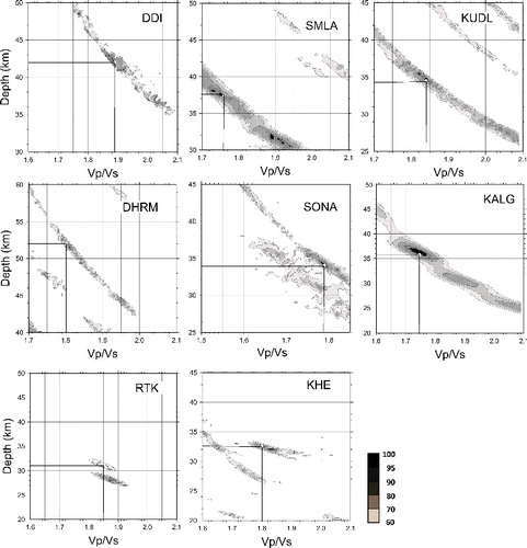
Better crustal composition interferences can be made from the Vp/Vs ratio and it is directly proportional to the elastic parameter Poisson ratio ‘σ’ (equation A6(A6) ). Tarkov and Vavakin (1982) observed that increase of metamorphic grades has significant effects on the Vp/Vs ratio. They inferred that values of Vp/Vs for common crustal and mantle rocks lie between 1.73 and 1.87. The average crustal value of Vp/Vs (1.79) is slightly greater than the global average for the continental crust, but close to that expected for mafic crusts (Christensen & Mooney 1995; Zandt Ammon 1995).

4.3. Receiver function inversion to derive shear wave velocity structure

The receiver function can be inverted to obtain shear wave velocity structure beneath a given seismic station by minimizing the differences between observed and synthetic receiver functions (Ammon et al. 1990; Ammon 1991). The time domain radial receiver functions for all the eight stations are inverted by the linearized inversion technique to get the shear wave velocity structure under each site. As there is no guarantee that a unique inversion result will be obtained, we use a priori available information to constrain the equations. Here we used time domain iterative inversion using Haskell mathematics (Haskell 1962; Liggoria & Ammon 1999). In this technique, we have implicitly assumed an isotropic seismic structure of the upper mantle with flat planar interfaces. We utilized a priori information based on the velocity model given by Rai et al. (2006) and Kumar et al. (2009) for the Northwest Himalaya region and Srinagesh et al. (2011) for the Indian shield stations. The inverted velocity model is shown by red coloured lines along the initial model of blue coloured dashed lines (figures 7 and 8). A comparison between the synthetic and observed stacked radial receiver functions is shown on the right-hand side corresponding to the velocity model.

Figure 7. Shear wave velocity model at different stations located at Northwest Himalaya depicts clear Moho, shown on the left side. The red lines are generated by real observation and blue dashed lines are the predicted input model. The match of real and synthetic waveforms is shown in the right hand side for corresponding station's velocity model. The blue colored solid line represents synthetic waveform obtained from input model and red colored solid lines represents obtained from seismic data. To view this figure in colour, please see the online version of the journal.

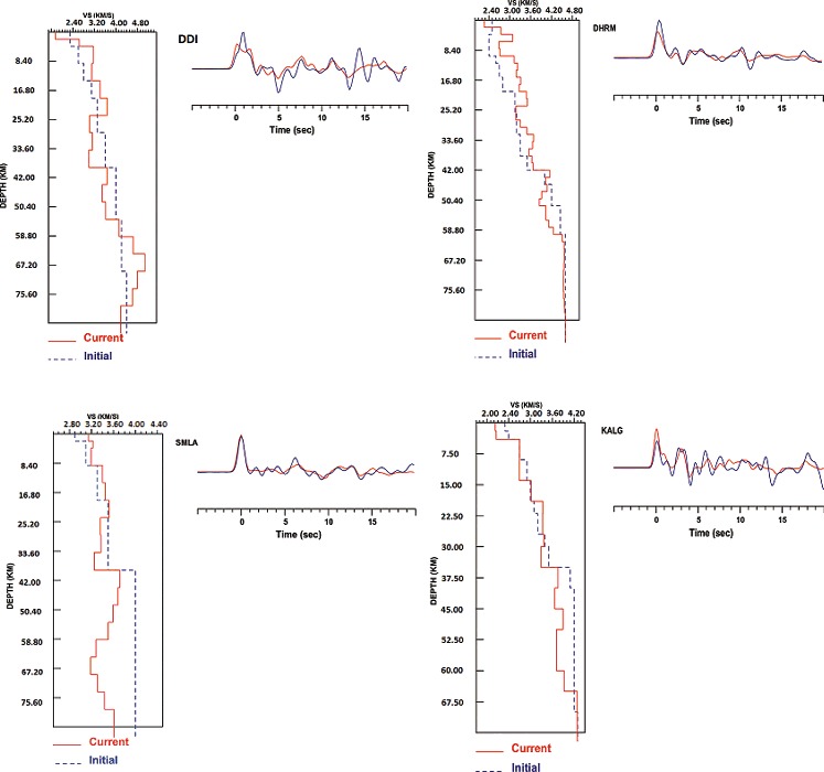
Figure 8. Shear wave velocity model at different stations located at Indo-Gangetic Plain. Description of the figure is same as figure 7.

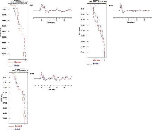
The DHRM station is the northernmost station situated in the Northwest Himalaya. At this site, there are sharp increases in the S-velocity from 2.2 to 3.1 km s⁻¹ at a depth of 5 km and 3.1 to 3.5 km s⁻¹ at a depth of 15 km. A low-velocity layer zone of 5 km width is observed at 7–11 km depth, where velocity drops from 3.1 to 2.7 km s⁻¹. After a depth of 25 km, there is a gradational increase in velocity upto 52 km depth. The Moho is observed at around 52 km depth and S-velocity of 4.0 km s⁻¹ is observed. The largest data-set of 105 events is recorded at the DDI station located at the Northwest Himalaya above the Indo-Gangetic plain. At the DDI site, the S-wave velocity is 2.1 km s⁻¹ near the surface and increases to 2.7 km s⁻¹ at 6 km depth and further increases to 3.2 km s⁻¹ at around 16 km depth. There is a low-velocity layer between 25 and 40 km where the velocity drops from 3.7 km s⁻¹ to 3.0 km s⁻¹. The Moho is observed at around 40 km with an S-wave velocity 4.1 km s⁻¹. The SMLA is situated on the HFT where Vs is around 3.1 km s⁻¹ near the surface and up to 10 km depth Vs is around 3.2 km s⁻¹. After 10 km depth, velocity increases to 3.5 km s⁻¹ and continued upto 24 km depth. There is a decay of S-velocity from 24 km to 37 km depth where the S-wave velocity is 3.2 km s⁻¹. The Moho is observed at around 37.5 km depth with an S-velocity increased to 3.8 km s⁻¹. The KALG station is located on the margin of the sub-Himalaya near the Indo-Gangetic plain. At this site Vs of 2.1 km s⁻¹ is observed upto a depth of 4 km. At the upper crust, Vs increases to 2.7 km s⁻¹ upto 14 km depth. Near a depth of 35.5 km the Vs sharply increases to 4.0 km s⁻¹, which is interpreted as the depth of Moho discontinuity. In the Indo-Gangetic plain (figure 8), KHE is the southernmost station situated on the alluvial plain. At this site, a low Vs of 1.4 km s⁻¹ is observed on the surface which increases to 2.4 km s⁻¹ at 2 km depth. The Moho discontinuity is observed at a depth of around 32.5 km. Station KUDL is located near the KHE station having a less number of recorded events. At this site, Vs is about 2.1 km s⁻¹ for the first 3 km depth and increases to 2.4 km s⁻¹ upto 8 km depth. There is no obvious velocity gradient in the upper and mid crusts of the KUDL station. The Moho is the pronounced discontinuity observed at 34 km depth with a shear wave velocity 3.6 km s⁻¹. Station SONA is located east of the KUDL station, exhibiting a simple shear wave velocity structure. The SONA station shows Vs of about 1.6 km s⁻¹ at the surface, which gradually increases to 3.5 km s⁻¹ at a depth of 34 km, which is interpreted as the Moho.

5. Discussions

The variation in the P-to-S conversion from the direct P-arrival time observed across the Northwest Himalaya and Indo-Gangetic plain is interpreted in terms of lateral variations of crustal thickness. The results from this study are generally in agreement with earlier studies (Caldwell et al. 2009; Kumar et al. 2009). The use of a single method for a large area facilitates a comparison between the shield region and foothills mountain region where active deformation is continuing. However, due to the non-uniqueness of the problem, a model close to the real structure can only be obtained through an integrated approach. A resolution of the order of 2–5 km in layer thickness is sufficient to resolve major changes in the velocity structure. The last 10 years seismicity observation of the Northwest Himalaya region reveals that the seismicity is concentrated at a shallow depth in between ∼10 and 20 km in the upper crust in the Northwest Himalayan region (Priestley et al. 2008; Yadav et al. 2009). A combination of the velocity gradients with varying Moho depth distributions presents a good approximation to the crustal structure on a regional scale and would help to improve earthquake locations.

Our result in the Northwest Himalaya region is in agreement with the Moho depths estimated by various authors (Rai et al. 2006; Kumar et al. 2009). A previous study by Kumar et al. (2009) determined a velocity model for the whole of the Northwest Himalaya region by travel time inversion and got an average Moho depth of 44 km. Our result in the same region shows an average Moho depth of around 40 km. Significantly, larger Moho depths in the range of 37–52 km are obtained for the SMLA, DDI and DHRM stations located in the Northwest Himalaya, but comparatively lesser depths in the range of 30–34 km are obtained at the stations located at the Indo-Gangetic plain (figure 9).

Figure 9. Map of the Moho depth variation below sea level using the value of ‘H’ from table 1. Values are obtained from Zhu and Kanamori (2000) techniques weighted for contour diagram. Seismic stations are represented by black solid triangles with station codes.

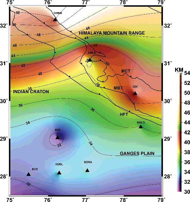
Figure 10. A. Map of distribution of Vp/Vs ratio obtained from H-K analysis for the study region. B. Cross section mapping of Vp/Vs derived from eight broadband stations from south to north of our study region.

Recently, Mechie and Kind (2013) observed the Moho variation and shear wave velocity structure along a 700-km-long profile transect through the High Himalaya near the Tibetan Plateau upto Golmud through the Qaidam, Tarim and Sichuan basins. They found about 10 km difference in the Moho depths between the Qaidam basin and Northern Tibetan plateau. We have found that the crust of the Siachuin and Tarim basins, similar to the Indo-Gangetic plain in terms of Moho depths (35–40 km), whereas at the Qaidam basin, the marginal part of the Northern Tibetan plateau, the Moho is deeper with a depth of 55 km. Stations DHRM, SMLA and DDI have Moho depths of 52 km, 37.5 km and 42 km, respectively, and the Moho depth decreases southwards as we move towards the Indo-Gangetic Plain with an average Moho depth of 33 km. The stations of the sub-Himalayan part, a low S-velocity anomaly is obtained within the mid crust similar to Kind et al. (2002) who inferred a low-velocity intra-crustal layer in the northern Tibet orogeny. Mechie and Kind (2013) correlated the crustal Poisson ratio with the crustal age contemporary to our study region of the tertiary period. We obtained lower to intermediate Poisson ratios (0.253–0.287) for the Indo-Gangetic Plain which is more or less similar to that of the Tarim and Sichuan basins with an average Poisson ratio of 0.270 (Wang et al. 2010).

In our present work, we observed a low velocity patch in the mid crust around 10 km thick layer in DDI station and much similar findings are also observed in DHRM and SMLA station. Arora et al. (2007) proposed a northeast dipping structure with low resistivity (∼30 Ω) from Mangnetotelluric study around this region. They concluded that this low velocity structure represents the Main Boundary Thrust or Himalayan Frontier Thrust (HFT) which represents sedimentary rocks overlying the under thrust Indian plate. Caldwell et al. (2013) cited that low S-wave velocity layer and low resistivity structure in the mid crust represents presence of melts or aqueous flow where high concentration of seismicity is observed in this sub-Himalayan part.

The crustal composition is closely related to the Vp/Vs ratio or equivalent to Poisson ratio. Mineralogy of rocks plays a key role in variation of Vp/Vs ratio. For lower crustal rocks, low Vp/Vs ratio (< 1.75) or low Poisson's ratio (σ<0.26) for the Mesozoic-Cenozoic crust is considered to indicate a predominantly felsic composition and intermediate σ (0.26–0.28) to high σ (> 0.28) are the characteristics for intermediate to mafic composition (Zandt & Ammon 1995; Christensen 1996; He et al. 2014, 2015).The Vp/Vs values are around 1.73 for felsic rocks, whereas for mafic rocks, Vp/Vs values tends to increase. The values of bulk crustal ratio are slightly less than lower crustal Vp/Vs ratio (about 0.02). So we can use the bulk Vp/Vs to determine the lower crustal Vp/Vs to get the composition of rocks (Christensen 1996; He et al. 2013). In general, the mafic rocks have high Poisson's ratio while the felsic rocks have low Poisson's ratio, due to their different mineral contents like quartz, feldspar and plagioclase. An increase of plagioclase content and a decrease of quartz content can explain by the increase of Poisson's ratio while the felsic rock have low Poisson's ratio for the abundance of quartz content (Chevrot & van der Hilst 2000). The prominent variation in crustal thickness and Poisson's ratio across our study region reflects the complexity of the geological structure and crustal composition. The medium to high values for Vp/Vs ratio (1.740–1.890) across the Mesozoic to Cenozoic formation of sub Himalaya and foothill region are characterized by intermediate to mafic-ultramafic of lower crust.

Ni and Barazangi (1984) concluded that the whole Himalaya belt is characterized by an interconnected network of extensional fracture and normal faults and fractured portions are filled with fluids, which results in high Vp/Vs ratios in the region. The Poisson's ratio estimated in the present study for Northwest Himalaya and adjoining regions shows heterogeneity in the crustal composition and existence of partial melts in some parts (table 1). Most of the stations (DHRM, SMLA, KALG, KUDL, KHE, and SONA) has an intermediate to high Poisson ratio (> 0.25). The ratio is high for DDI station (> 0.30) located in the Northwest Himalaya. The medium-to-high value in the Northwest Himalaya region are consistent with a mafic/ultramafic lower crust as inferred from other geophysical surveys (Gokarn et al. 2002; Arora et al. 2007).

6. Conclusion

The results obtained from P wave receiver functions and other geophysical studies suggest that the collision zone of sub Himalaya is characterized by a crust with an average depth of about 40 km. Data from eight seismic stations shows that the depth of Moho increases from Indo-Gangetic plain deepens towards lesser Himalaya where maximum Moho thickness of 52 km is obtained at Dharamsala site. Velocity modeling for all stations shows heterogeneity of the crust in the Northwest Himalaya as well as Indian shield region. The most prominent observation from the inversion of S-wave velocity at many stations in the Northwest Himalaya shows the presence of low velocity zone (LVZ) around 10 to 35 km in different thickness patches in which seismicity is concentrated. The main reason of LVZ may be due to the presence of fluids trapped in highly fractured rocks well justified by high Vp/Vs in the inner portion of the sub Himalayan arc. The concentration of high Vp/Vs ratio or high Poisson ratio (≥0.260) may also be due to the mafic or ultra-mafic composition in the middle to lower crust of lower Himalayan region. Conversely, no prominent LVZ is observed in the stations located in the Indo-Gangetic Plain. The medium to higher Vp/Vs values may reflects the hydrated sedimentary material subducted on the top of the Indian shield region. The crustal structure models developed from this study provided new information that can be used to refine the velocity model used in earthquake locations for the region, thus increasing the knowledge of the current seismicity of the sub Himalaya as well as Indian shield region and enabling more detailed seismic hazard studies to be carried out.

Acknowledgments

We sincerely thank technical persons of India Meteorological Department in maintaining and data archival of stations we used in our analysis. Authors like to express deep sense of gratitude to Prof. Chuansong He and an anonymous reviewer and thankfully acknowledged for their extremely insightful comments. The GMT software package distributed by Wessel and Smith (1995) was used for mapping purpose.

Disclosure statement

No potential conflict of interest was reported by the authors.

References

- Ammon CJ. 1991. The isolation of receiver effects from the teleseismic P waveforms. Bull Seismological Soc Am. 81:2504–2510.
- Ammon CJ, Randall GE, Zandt G. 1990. On the non-uniqueness of receiver function inversions. J Geophysical Res. 95:15303–15318.
- Arora BR, Unworth MJ, Rawat G. 2007. Deep resistivity structure of the northwest Indian Himalaya and its tectonic implications. Geophys Res Lett. 34:L04307. doi:10.1029/2006GL029165.
- Besse J, Courtillot C. 1988. Paleogeographic maps of the continents bordering the Indian Ocean since the Early Jurassic. J Geophys Res. 93:11791–11808.
- Bilham R, Gaur VK. 2000. Geodetic contribution to the study of seismotectonics in India. Curr Sci. 79:1259–1269.
- Bilham R, England P. 2001. Plateau ‘pop-up’ in the great 1897 Assam earthquake. Nature. 410:806–809.
- Bollinger L, Avouc JP, Cattin R, Pandey MR. 2004. Stress buildup in the Himalaya. J Geophys Res. 209:B11405, doi: 10.1029/2003JB002911.
- Caldwell WB, Klemperer SL, Lawrence JF, Rai SS, Ashish. 2013. Characterizing the main Himalayan thrust in the Garhwal Himalaya, India with receiver function CCP stacking. Earth Planet Sci Lett. 367:15–27.
- Caldwell WB, Klemperer SL, Rai SS, Lawrence JF. 2009. Partial melt in the upper-middle crust of the northwest Himalaya revealed by Rayleigh wave dispersion. Tectonophysics. 477:58–65.
- Chevrot S, Van Der Hilst RD. 2000. The Poisson ratio of the Australia crust: geological and geophysical implications. Earth Planet Sci Lett. 183:121–132.
- Christensen NI. 1996. Poisson ratio and crustal seismology. J Geophys Res. 101:3139–3156.
- Christensen NI, Mooney WD. 1995. Seismic velocity structure and composition of the southern Italy. Geophys Res Lett. 31:L07615, doi: 10.1029/2004GL019480.
- Fu B, Lin A. 2003. Spatial distribution of the surface rupture zone associated with the 2001 Ms 8.1 Central Kunlun earthquake, northern Tibet, revealed by satellite remote sensing data. Int J Remote Sens. 24:2191–2198.
- Gitis V, Yurkov E, Arora BR, Chabak S, Kumar N, Baidya P. 2008. Analysis of seismicity in North India. Russian J Earth Sci. 10:ES5002, doi: 10/2205/2008ES000303.
- Gokarn SG, Gupta G, Rao CK, Selvaraj C. 2002. Electrical structures across the Indus Tsangpo suture and shyok suture zones in NW Himalaya using Magnetotelluric studies. Geophys Res Lett. 29:92-1–92-4 .
- Guillot S, Maheo G, de Sigoyer J, Hattori KH, Pecher A. 2008. Tethyan and Indian subduction viewed from the Himalaya high to ultrahigh-pressure metamorphic rocks. Tectonophysics. 451:225–241.
- Gurrola H, Baker GE, Minster JB. 1995. Simultaneous time domain deconvolution with application to the computation of receiver functions. Geophysics J Int. 120:537–543.
- Harinarayana T, Abdul Azeez K, Naganjaneulu K, Manoj C, Veeraswamy K, Murthy D, Prabhakar Eknath Rao S. 2004. Magnetotulluric studies in Puga valley geothermal field, NW Himalaya, Jammu and Kashmir, India. J Volcanology Geothermal Res. 138:405–424.
- Haskell NA. 1962. Crustal reflection of plane P and SV wave. J Geophysics Res. 67:4751–4767.
- He C, Dong S, Chen X, Santosh M, Li Q. 2014. Crustal structure and continental dynamics of Central China: A receiver function study and implications for ultrahigh-pressure metamorphism. Tectonophysics. 610:172–181.
- He C, Dong S, Santosh M, Chen X. 2013. Seismic Evidence for a Geosuture between the Yangtze and Cathaysia Blocks, South China. Sci Rep. 3:2200, doi: 10.1038/srep02200.
- He C, Santosh M, Dong S. 2015. Continental dynamics of Eastern China: Insights from tectonic history and receiver function analysis. Earth-Sci Rev. 145:9–24.
- Jade S. 2004. Estimates of plate velocity and crustal deformation in the Indian subcontinent using GPS geodesy. Curr Sci. 86:1443–1448.
- Kayal JR. 2001. Microearthquake activity in some parts of the Himalaya and the tectonic model. Tectonophysics. 339:331–351.
- Kayal JR. 2007. Recent large earthquakes in India: seismotectonic perspective. IAGR Memoir. 10:189.
- Kind R, Kosarev GL, Petersen NV. 1995. Receiver functions of the stations of the German regional seismic network (GRSN). Geophysical Int. 121:191–200.
- Kind R, Yuan X, Saul J, Nelson D, Sobolev SV, Mechie J, Zhao W, Kosarev G, Ni J, Achauer U, Jiang M. 2002. Seismic images of crust and upper mantle beneath Tibet: Evidence for Eurasian plate subduction. Science. 298:1219–1221.
- Kumar N, Sharma J, Arora BR, Mukhopadhyay S. 2009. Seismotectonic model of the Kangra-Chamba of Northwest Himalaya: Constraints from joint hypocenter determination and focal mechanism. Bull Seismological Soc Am. 99:95–109.
- Langston CA. 1977. The effect of planar dipping structure on source and receiver responses for constant ray parameter. Bull Seismol Soc Am. 67:1029–1050.
- Ligorria JP, Ammon CJ. 1999. Iterative deconvolution and receiver-function estimation. Bull Seismological Am. 89:1395–1400.
- Mechie J, Kind R. 2013. A model of the crust and mantle structure down to 700 km depth beneath the Lhasa to Golmud transect across the Tibetan plateau as derived from seismological data. Tectonophysics. 606:182–197.
- Molnar P, Fitch TJ, Wu FT. 1973. Fault plane solution of shallow earthquakes and contemporary tectonics in Asia. Earth Planetary Sci Lett. 19:101–112.
- Molnar P, Tapponiar P. 1975. Cenozoic tectonics of Asia: Effects of continental collision. Science. 189:419–426.
- Ni J, Barazangi M. 1984. Seismotectonics of the Himalayan collision zone: geometry and under thrusting Indian plate beneath the Himalaya. J Geophysical Res. 89:1147–1163.
- Owens TJ, Zandt G, Taylor SR. 1984. Seismic evidence for an ancient rift beneath the Cumberland Plateau, Tennessee: A detailed analysis of broadband teleseismic P waveforms. J Geophysical Res. 89:7783–7795.
- Ozalaybey S, Savage MK, Sheehan AF, Louie JN, Brune JN. 1997. Shear wave velocity structure in the northern Basin and Range province from the combined analysis of receiver functions and surface waves. Bull Seismological Soc Am. 87:183–199.
- Pandey MR, Tadukar RP, Avouac JP, Vergne J, Heritier T. 1995. Interseismic strain accumulation on the Himalaya crustal ramp. Geophysics Res Lett. 22:741–754.
- Priestley K, Jackson J, McKenzie D. 2008. Lithospheric structure and deep earthquakes beneath India, the Himalaya and southern Tibet. Geophysics J Int. 172:345–362.
- Rai, SS, Priestly K, Gaur VK. 2006. Configuration of the Indian Moho beneath the NW Himalaya and Ladakh. Geophysical Res Lett. 33:L15308.
- Seeber L, Armbruster JG, Quimeyer R. 1981. Seismicity and continental subduction in the Himalayan Arc. In: Gupta HK, Delany FM, editor, Zagros, Hindu Kush, Himalaya, geodynamic evolution, geodynamic series, vol. 3. Washington D C: America Geophysical Union; p. 215–242.
- Srinagesh D, Singh SK, Chadha RK, Paul A, Suresh G, Ordaz M, Dattatrayam RS. 2011. Amplification of seismic waves in the Central Indo-Gangetic Basin, India. Bull Seismol Soc Am. 101:2231–2242.
- Tarkov AP, Vavakin VV. 1982. Poisson's ratio behavior in crystalline rocks: Application to the study of the Earth's interior. Phys Earth Planetary Int. 29:24–29.
- Vinnik LP. 1977. Detection of waves converted from P to SV in the mantle. Phys Earth Planetary Int. 15:39–45.
- Wadia DN. 1931. The syntaxis of the northwest Himalaya: its rocks, tectonics and orogeny. Rec Geol Surv India. 65:189–220.
- Wang CY, Zhu L, Lou H, Huang BS, Yao Z, Lou X. 2010. Crustal thickness Poission's ratio in the Eastern Tibetan Plateau and their tectonic implication. J Geophysics Res. 115:B11301.
- Wessel P, Smith, WHF. 1995. New version of the generic mapping tools released. EOS Trans. AGU, 76:329.
- Yadav DK, Kumar N, Paul P. 2009. Recent seismicity and stress pattern in NW Himalaya. Himalayan Geol. 30:139–145.
- Yin A. 2006. Cenezoic tectonic evolution of the Himalayan orogen as constrained by along strike variation of structural geometry, exhumation history, and foreland sedimentation. Earth-Sci Rev. 76:1–131.
- Yuan X, Ni J, Kind R, Mechi J, Sadvol E. 1997. Lithosphere and upper mantle structure of southern Tibet from a passive source experiment. J Geophysical Res. 102:27,491–27,500.
- Yuan X, Sobolev SV, Kind R. 2001. Moho topography in the central Andes and its geodynamic implication. Earth Planetary Sci Lett. 199:389–402.
- Yuan X, Sobolev SV, Kind R, Oncken O, Andes Seismology Group. 2000. New constraint on subduction and collision process in the central Andes from comprehensive observations of P to S converted seismic phase. Nature. 408:958–961.
- Zandt G., Ammon CG. 1995. Continental crust composition constrains by measurements of crustal Poisson's ratio. Nature. 374:152–154.
- Zhang Y, Feng, WP, Xu, LS, Zhou CH, Chen YT. 2009. Spatio-temporal rupture process of the 2008 great Wenchuan earthquake. Sci China Ser D Earth Sci. 52:145–154.
- Zhu L, Kanamori H. 2000. Moho depth variations in southern California from receiver functions. J Geophysical Res. 105:2969–2980.