Retrieval and application of leaf area index over China using HJ-1 data

ABSTRACT

Although leaf area index (LAI) is one of the essential parameters employed to monitor global vegetation, no global LAI products which use a fine spatial resolution yet exist. To remedy this, we herein outline an adapted LAI retrieval algorithm which employs HuanJing-1 charge-coupled device (HJ-1 CCD) data, which was originally determined using Landsat thematic mapper (TM) data. Validation of this adapted LAI retrieval algorithm via field measurements demonstrates that errors for ∼72% of the sample sites were within a range of 0.2 for the Bashang Grassland in Hebei Province, and within 1.0 for the Taihe region in Jiangxi Province. In addition, the correlation coefficients (R) of HJ-1 LAI and ground-measured LAI data were similar to those of MODIS LAI and ground-measured LAI datasets for both regions. These results demonstrate the potential for transposing a mature Landsat LAI-retrieval algorithm to HJ-1 data. Furthermore, we generated 30 m HJ-1 LAI datasets for China for the summer of 2012. An analytical comparison between retrieved HJ-1 LAI and MODIS LAI data showed the coherence of the LAI distribution. Finally, a specific post-forest fire area was mapped using HJ-1 LAI datasets.

KEYWORDS:

• Leaf area index (LAI)
• HJ-1 CCD
• Landsat5 TM
• vegetation distribution
• burned area mapping

1. Introduction

LAI is defined as one-half of the total green leaf area per unit of horizontal ground surface area (Chen & Black 1992). LAI, which is an indicator of plant foliage density, is one of the essential parameters used in any assessment of the global ecosystem, the quantification of the hydrological/carbon cycle and climate change modeling (Sellers et al. 1997; Keller et al. 2001). LAI retrieved from remote-sensing data is effective in the monitoring of global vegetation. There are two principal methods used to estimate LAI from satellite data. The first is the statistical model which utilizes the empirical relation between field LAI measurements and vegetation indices like the normalized difference vegetation index (NDVI), built upwards from ground measurements to remote-sensing data (Thenkabail et al. 1994; Thenkabail 2003; Duchemin et al. 2006). However, this model relies on the calculation of the specific canopy spectral properties, soil backgrounds and spatial distributions of leaves (Chen et al. 2002), limiting its applicability to any global retrieval of LAI values. The second method establishes a physically based relation between canopy reflectance and the LAI value, based on modelled simulations such as canopy radiative transfer, geometric-optical or hybrid modeling (the latter being a combination of the canopy radiative transfer and geometric-optical models). Such models based on physical vegetative processes are built on various vegetative environments, and thus can be widely used. The retrieval of inverse LAI data from radiative transfer models is based on iterative techniques (Walthall et al. 2004). The Look-Up-Table (LUT) is one commonly used iterative technique, and is based on prior-simulated reflectance datasets and the minimizing of any cost function iterations (Myneni et al. 1989; Colombo et al. 2003; Zheng & Moskal 2009; Liang et al. 2013a, Zhu et al. 2013).

There are sufficient coarse spatial resolution LAI products, such as MODIS LAI (Myneni et al. 2002; Huang et al. 2008), CYCLOPES and GLOBCARBON LAI (Baret et al. 2007; Weiss et al. 2007), GLASS LAI (Liang et al. 2013b) and AVHRR GIMMS LAI3 (Zhu et al. 2013). All these are very important for monitoring global environmental changes. However, fine spatial resolution products are required to address patch or regional-scale scientific studies for a more accurate assessment of local ecosystems, crop yield estimation, forest fire mapping, etc.

Remote-sensing data such as Landsat TM and HJ-1 CCD data with 30 m spatial resolution are good sources for producing a LAI product with a fine spatial resolution. Several studies have already tried to obtain a global LAI product using Landsat datasets. For example, Ganguly et al. (2010, 2012) developed a new algorithm based on the radiative transfer model and the canopy spectral BRF model. Gao et al. (2014) developed an improved regression tree mapping approach. There have been several attempts to retrieve LAI data by employing the HJ-1 CCD datasets for some specific vegetation types as part of an empirical method, such as those proposed by Chen et al. (2010) for shrubs, Yang et al. (2013) for grasses, Zhang et al. (2010) for rice etc. HJ-1 CCD is onboard the Environment and Disaster Monitoring and Predicting Small Satellite constellation, which contains two small optical satellites (HJ-1A and HJ-1B) (Wang et al. 2010) and has a wider scanning swath than Landsat TM (the detailed spectral parameters can be found in Table 1). Thus, HJ-1 CCD has the advantage of a quick global coverage in two days, while Landsat TM takes 16 days to cover the globe. HJ-1 CCD data are therefore promising for the development of a higher spatial and temporal resolution LAI product which is more meaningful for vegetation monitoring. It has therefore become necessary to develop an operational method for HJ-1 CCD to allow the retrieval of a global LAI.

Table 1. Spectral parameter characteristic of Landsat TM and HJ-1 CCD sensors.

Sensor	Band number	Spectral region (μm)	Spatial resolution (m)	Return period (d)	Scene width (km)
Landsat TM	1 (Blue)	0.45–0.52	30	16	185
	2 (Green)	0.52–0.60	30
	3 (Red)	0.63–0.69	30
	4 (NIR)	0.77–0.90	30
HJ-1 A/B CCD	1 (Blue)	0.43–0.52	30	4	360 (single CCD)
	2 (Green)	0.52–0.60	30
	3 (Red)	0.63–0.69	30		720 (double CCDs)
	4 (NIR)	0.76–0.90	30

Natural disasters such as flood, drought, earthquake and forest fires occur frequently in China, and have a severe impact on the local ecological environment and economy. Based on high resolution remote-sensing data, we can obtain environmental information about the ground surface which can, for example, allow the accurate mapping of particular areas and help more effective disaster assessment and post-disaster reconstruction. Some new indices and disaster mapping have already been generated using such HJ-1 or Landsat data. For example, Jung et al. (2014) used Landsat data to map flood inundations areas, Chen et al. (2016) and Liu et al. (2016) used Landsat and HJ-1 data to map burned forest areas, separately, and Xing and Hu (2016) performed similar work in extracting marine plant and disaster information using both HJ-1 and Landsat data. In this study, the LAI retrieval algorithm originally developed for the Landsat TM by Ganguly et al. (2012) was applied to retrieve HJ-1 CCD LAI, as the similarity between HJ-1 CCD and Landsat TM data allows the possibility of transplanting the Landsat TM algorithm to HJ-1 CCD data. Based on this method, a LAI product for all China for the summer of 2012 was developed.. Furthermore, this product was used to help generate a post-fire burned area map for one specific fire site. Forest fires are critically serious natural disasters with a huge destructive potential. Such fires therefore need to be effectively monitored. Burned areas need to be accurately mapped to allow the effective calculation of both ecological and economic losses attendant upon such natural disasters. Additionally, such data can help facilitate effective reforestation programmes. Using the higher spatial and temporal resolution LAI product derived from HJ-1 CCD data, it has become possible to map post-fire burned areas more accurately, and in particular to detect changes in the area affected by fire during the fire events themselves.

The aim of this study was to derive a 30m HJ-1 LAI dataset, and thereby produce a 30m HJ-1 LAI map of China. As a case study, we selected one forest fire site in 2012 and used the new HJ-1 LAI dataset to help map the burned area. We describe the studied regions and data collection method used in Section 2 and present our retrieval method in Section 3. In Section 4, we investigate the potential transposition of the LAI retrieval algorithm originally designed for Landsat data to the HJ-1 dataset. A LAI map for China for the summer of 2012 is then obtained using HJ-1 data and evaluated by applying the MODIS LAI products. The applicability of HJ-1 LAI data to post-fire burned area mapping is then verified. Section 5 we make a summary of the study and look ahead.

2. Data

Land-cover data and LAI products from MODIS instruments, Landsat TM data, HJ-1 CCD data and LAI field measurements were used to evaluate the retrieval algorithm. MODIS LAI and vegetation distribution data were adopted to evaluate the values of 30m HJ-1 LAI data. All remote-sensing data were projected on to the GCS Lat/Lon projection. Moreover, two study regions in China (the Bashang Grassland in Hebei Province and the Taihe region in Jiangxi Province) were chosen for field validation of the accuracy of HJ-1 LAI retrieved data, and a forest fire site (Yimen County in Yunnan Province) was selected for burned area mapping.

2.1. MODIS Products

Two multi-day tiled MODIS products (MCD12Q1 and MOD15A2) were used in this study. MOD15A2 is a MODIS LAI product composed globally over an eight-day cycle with a 1 km spatial resolution; this was then compared with the HJ-1 LAI for the study regions. MCD12Q1 is a C5 MODIS Land Cover Type product (Friedl et al. 2010) with a spatial resolution of 500 m, and was used to identify vegetation types in the study regions. This MODIS Land Cover Type product provides eight biome types, including grass, shrubs, crops, savanna, deciduous broadleaf forest (DBF), evergreen broadleaf forest (EBF), deciduous needleleaf forest (DNF) and evergreen needleleaf forest (ENF), using the MODIS LAI/PAR biome classification algorithm. The mosaic produced by MCD12Q1 over China (2012) was resampled to a 30 m spatial resolution.

2.2. HJ-1 CCD data

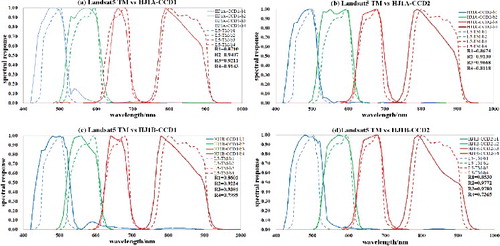
HJ-1 A/B raw data were obtained from the China Centre for Resources Satellite Data and Application (CRESDA). The spectral wavelengths of HJ-1 A/B CCD bands (blue, green, red and shortwave infrared) are 0.43–0.52 μm, 0.52–0.60 μm, 0.63–0.69 μm and 0.76–0.90 μm, respectively. The CCD cameras on the HJ-1 satellites have a nadir pixel resolution of 30m, a width of view of 360 km and a central-pixel matching accuracy of 0.3 pixels. As shown in Table 1, the wavelengths and bandwidths of the four HJ-1 A/B CCD bands are almost the same as those of the first four bands of the Landsat TM. In addition, the spectral reflectance of the four multispectral bands of HJ-1 CCD are clearly consistent with those of the Landsat TM sensors, with most R (labelled as R1 for the blue band, R2 for the green band, R3 for the red band and R4 for the NIR band) ≥ 0.8 (Figure 1). The red reflectance of HJ-1 CCD generated a higher correlation with the Landsat TM sensor. The red and NIR band reflectances between the two sensors were highly correlated, with high R values. For example, the correlations between HJ-1 CCD1 and Landsat TM were R3 = 0.9211 and R4 = 0.9143, and the correlations between HJ-1 CCD2 and Landsat TM were R3 = 0.9668 and R4 = 0.8118.

Figure 1. Relative spectral responses for the various spectral bands of the HJ-1 CCD and Landsat TM sensors.

Using the MODIS LAI/PAR classification system, 221 HJ-1 CCD images for eight stochastic homogeneous regions were collected over China during the summer of 2012. To fill any gaps in the data caused by cloud cover or missing data, data from the year before and year following were used.

2.3. Landsat TM data

The consistency between the spectral response reflectances of the first four multispectral bands of both HJ-1 and Landsat data have already been described in Section 2.2. Landsat data were used to evaluate further the comparability of land surface reflectances between HJ-1 and Landsat datasets in order to test the feasibility of the HJ-1 data LAI retrieval algorithm. Landsat imageries were acquired from the United States Geological Survey (USGS). The data acquisition period used in this paper was the summer leaf-on period from 2009 to 2011. This period was used because there were no Landsat data available for the period November 2011 to April 2013 due to instrument anomalies and updating. Landsat surface reflectance data were derived from top-of-atmosphere (TOA) reflectance values using the Landsat Ecosystem Disturbance Adaptive Processing System (LEDAPS) for calibration and atmospheric correction (Masek et al. 2006).

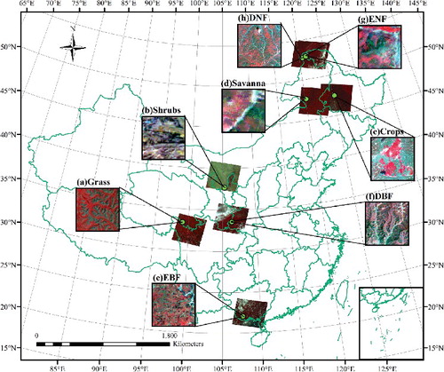
Landsat surface reflectance data and the corresponding HJ-1 reflectance data, which represent biome-specific homogeneous regions with reference to MODIS land cover vegetation type products, are listed in Table 2. The location of the scenes is shown in Figure 2. The acquisition date differences between HJ-1 images and the corresponding Landsat TM images were within two days, assuming that there were minimal land surface phenological changes during a two-day period.

Table 2. HJ-1 and Landsat TM images selected for varying biome reflectance/LAI comparison.

Biome type	HJ-Sensor	Path	Row	Acquisition date	Landsat-sensor	Path	Row	Acquisition date
Grass	HJ1A-CCD1	20	76	Aug/15/2010	TM	133	37	Aug/14/2010
Shrubs	HJ1B-CCD2	14	68	Jun/22/2010	TM	130	34	Jun/22/2010
Crop	HJ1A-CCD1	450	57	Jun/26/2010	TM	119	27	Jun/25/2010
Savanna	HJ1B-CCD1	455	56	Aug/10/2011	TM	123	27	Aug/11/2011
Evergreen Broadleaf Forest (EBF)	HJ1B-CCD1	5	90	Jul/10/2009	TM	126	45	Jul/9/2009
Deciduous Broadleaf Forest (DBF)	HJ1A-CCD1	12	74	Jul/10/2010	TM	128	37	Jul/10/2010
Evergreen Needleleaf Forest (ENF)	HJ1B-CCD1	457	49	Jun/21/2010	TM	123	23	Jun/21/2010
Deciduous Needleleaf Forest (DNF)	HJ1B-CCD1	456	49	Jun/24/2011	TM	123	23	Jun/24/2011

Figure 2. Pure pixel stochastic blocks for eight biome types in China.

2.4. FROM-GLC data

As using only MODIS Land Cover data from a coarser resolution (500m) to a finer one (30m) would be likely to generate errors through the lack of a detailed structure and variability, 30m resolution global land cover products generated from 30m satellite data have the potential to improve the accuracy of land cover classification.

Finer Resolution Observation and Monitoring of Global Land Cover (FROM-GLC) data (Gong et al. 2013) have allowed the first 30 m resolution global land cover maps using Landsat TM and enhanced thematic mapper plus (ETM+) data to be produced. The data can be viewed and downloaded at http://data.ess.tsinghua.edu.cn/.

2.5. Field data

Validation of the HJ-1 LAI results for China using ground measurements is both difficult and complicated. Here, ground-measured LAI values determined with a LAI-2200 Plant Canopy Analyser for selected regions, including the Bashang Grassland and the Taihe region, were used for further validation.

The Bashang Grassland is located in Zhangbei County in northeastern Hebei Province (40.95–41.56°N, 114.17–115.45°E). The climate is temperate continental monsoonal; the region's mean altitude above sea level, mean annual temperature (MAT), mean annual precipitation (MAP) and mean frost-free period are 1400–1600 m, 2.6 °C, 300 mm and 90–100 d, respectively. The dominant land cover biome types are grass and crops. The Taihe region is situated in Jiangxi Province (26.45–26.97°N, 114.29–115.33°E). This region has a subtropical monsoonal climate; its mean altitude above sea level, MAT and MAP are 100 m, 17.9 °C, and 1489 mm, respectively. The dominant land cover vegetation types are coniferous forests composed of trees such as Pinus elliottii, Masson pine, and Cunninghamia lanceolata Hook.

The quadrats for ground measurement were designed to be 30 m × 30 m square in order to match the spatial resolution of the HJ-1 instrument. The time period selected for taking in-situ LAI measurements for investigation was 27 June–30 June 2012 for 25 sample sites in the Bashang Grassland, and 2 December–4 December 2012 for 32 sample sites in the Taihe region.

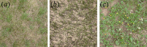
As in-situ data are just point values, there are always going to be observation-scale discrepancies between satellite and ground data. It was therefore critical that attention was paid to the surface homogeneity of the field quadrats in the two validation regions. Figure 3 shows sample plot examples of ground surface homogeneity in the Bashang Grassland.

Figure 3. Sample plots with surface homogeneity in the Bashang Grassland.

3. Methods

3.1. Data pre-processing

Data pre-processing includes geometric and atmospheric correction, as described in detail below.

• Geometric correction

The geometric correction method is the classic Ground Control Points (GCPs) method that uses Landsat TM images as standard reference imagery. In our study, a polynomial method was used to establish the relation between distorted images and standard reference images, and then the distorted images were warped. The geo-location warping error was limited to within half of a pixel.

• Radiation calibration and atmospheric correction

The true surface reflectance can be obtained from the DN value following three steps: (1) calibrating DN to the at-sensor spectral radiance; (2) converting spectral radiance to TOA reflectance; and (3) correcting to surface reflectance from TOA reflectance utilizing an atmospherically corrected approach.

1. Calibration and conversion to radiance.

For HJ-1 CCD images, the radiance L was calculated with the gains and offset values provided in the supplementary data record file using Equation (1)(1) $L=DN/Gain+Offset$(1) , where Gain and Offset values were taken as the conversion coefficient.(1) $L=DN/Gain+Offset$(1)

For Landsat TM images, the radiance L was calculated in Equation (2)(2) $L =\mathrm{ }(LMAX-LMIN)/(QCALMAX-QCALMIN)\times \left(QCAL-QCALMIN\right)+LMIN$(2) , where QCAL is the quantized calibrated pixel value in DN, QCALMAX and QCALMIN are the maximum and minimum quantized calibrated pixel values in DN, respectively, and LMAX and LMIN (W•m⁻²•sr⁻¹•μm⁻¹) are the calibration factors which are fixed for each spectral band.(2) $L =\mathrm{ }(LMAX-LMIN)/(QCALMAX-QCALMIN)\times \left(QCAL-QCALMIN\right)+LMIN$(2)

1. Radiance to reflectance.

TOA spectral radiance values were corrected to earth surface reflectance using the Second Simulation of the Satellite Signal in the Solar Spectrum (6S) methodology (Vermote et al. 1997). The key control of atmospheric correction is the aerosol optical depth (AOD), which can be obtained either by ground-based measurement systems such as AERONET or satellite products fitted with difference algorithms (Mei et al. 2012, 2014). The 6S model is an accurate atmospheric reflectance transfer model which describes the atmospheric effect of illumination propagation during the sun-target-sensor routine in different situations.

3.2. LAI data retrieval from Landsat

The radiative transfer-based retrieval approach for LAI estimation (Ganguly et al. 2010, 2012; Zhang et al. 2014) used by Landsat is the LUT method. It utilizes the red and NIR channels, land cover types from the National Land Cover Database (NLCD) and resampled MODIS 30m Land Cover Data as its critical input variables.

The algorithm first builds biome-based LUTs using a stochastic radiative transfer equation (Huang et al. 2008). These LUTs are a set of simulated BRF values computed on the basis of the canopy spectral invariants theory for varying LAI and sun/view geometries. A simulated LAI can therefore be obtained by fitting the analytical approximations with the input for a given group of variables of sun/view geometries and BRFs.

3.3. LAI data retrieval from HJ-1

The similarities between the spectral band characteristics of HJ-1 CCD and Landsat TM sensors have already been described. A LAI retrieval algorithm would therefore have great potential for LAI retrieval from HJ-1 reflectance data. Landsat LUTs were thus directly used in the HJ-1 LAI retrieval process.

The MODIS 500m land cover data employed were first resampled from a coarser resolution (500 m) to a finer one (30 m). As a lack of a detailed structure would be likely to produce errors, FROM-GLC data were employed to make up for any possible deficiency. The HJ-1 LAI retrieval process is described diagrammatically in Figure 4.

Figure 4. Schematic diagram describing the process of 30 m LAI retrieval from HJ-1 CCD data.

3.4. Burned-area extraction from HJ-1 LAI data

Previous studies have predominantly used thermal data to map burned areas (Giglio 2007), employing spectral indices such as the NDVI, the Burned Area Index (BAI) and the Global Environmental Monitoring Index (GEMI) (Chuvieco et al. 2002, 2008, García et al. 2014) based on visible and near infrared bands, or the Normalized Burn Ratio (NBR) (Yu & Chen 2015) based on visible, near infrared and shortwave infrared bands. Moreover, these methods have commonly used moderate- to low-resolution satellite sensors such as MODIS and AVHRR. Such sensors can map comparatively cheaply, but are less accurate on a local scale. We have therefore attempted to find a methodology for mapping on a local scale more accurately using a HJ-1 LAI. This index is based on purely visible and near infrared bands and is less susceptible to error accumulation. It can also use high-resolution temporal HJ-1 CCD data to reveal changes in burned areas during ongoing forest fire events.

In order to extract the burned area, we first derived HJ-1 LAI values from post-fire HJ-1 data, and then evaluated the effectiveness of the discrimination between the burned and unburned surfaces quantitatively using discrimination index M. A support vector machine (SVM) classifier was then applied to extract the burned area. Finally, we assessed the overall accuracy of the extracted result using the Kappa coefficient.

The discrimination index M (Veraverbeke et al. 2011) was calculated using Equation (3)(3) $M =\left|({\mu }_b-{\mu }_u)/({\sigma }_b-{\sigma }_u)\right|$(3) , where ${\mu }_b$ and ${\mu }_u$ were the mean LAI values for the burned area and the unburned area, respectively, and ${\sigma }_b$ and ${\sigma }_u$ were the standard deviations in the LAI for the burned area and the unburned area, respectively.(3) $M =\left|({\mu }_b-{\mu }_u)/({\sigma }_b-{\sigma }_u)\right|$(3)

Previous studies (Pereira et al. 1999; Veraverbeke et al. 2011) have shown that the discrimination between burned and unburned areas is better if the value of M is higher. In order to obtain the value of M, a burned area map needs to be generated using a maximum likelihood classifier. If the value of M is higher than one, it gives a clear discrimination, allowing HJ-1 LAI data to help extract the burned area more accurately. Moreover, the referenced burned area that could be regarded as the ‘true burned area’ can be more easily obtained using a maximum likelihood classifier and visual interpretation based on the HJ-1 reflectance data before and after the forest fire.

SVM is a supervised machine learning method used to carry out a supervised classification based on statistical learning theory; it is based on the principle of structural risk minimization (SRM) (Cortes & Vapnik 1995). Previous studies (Zammit et al. 2006; Petropoulos et al. 2011; Mallinis & Koutsias 2012) have shown that an SVM classifier operated better than most other classifiers using just the original Landsat TM data. As HJ-1 LAI data can distinguish vegetation cover more accurately, we used an image-based SVM classifier and combined this with HJ-1 reflectance and HJ-1 LAI values to classify images into burned areas and unburned areas.

Classification accuracy, a confusion matrix containing the overall error, and the kappa coefficient, were used to determine the accuracy of the SVM classifier and the discrimination potential of the HJ-1 LAI data.

4. Results and discussions

In order to demonstrate the availability of the Landsat LAI retrieval algorithm for HJ-1 satellite data, a comparison between the spectral reflectance and retrieved LAI values of two sensors was conducted. We then validated HJ-1 LAI values with the in-situ measurements, and cross-validated these with MODIS LAI values. Finally, we obtained the HJ-1 LAI for the whole of China for the summer of 2012, and a forest fire site was selected to evaluate the retrieval algorithm's burned area extraction capabilities.

4.1. Comparison between aggregated HJ-1 reflectance/LAI and Landsat data

Two different LAI results were obtained from Landsat and HJ-1 data using the same retrieval algorithm when surface reflectance was taken as one input parameter. Due to these uncertainties in reflectance values, a comparison between, and analysis of, the consistency between the spectral reflectance and inversed LAI values for the eight biome types between the two sensors were performed on particular groups of pixels, as shown in Figures 5 and 6, respectively.

Figure 5. Reflectance comparison between HJ-1 CCD and Landsat TM data for eight biome types.

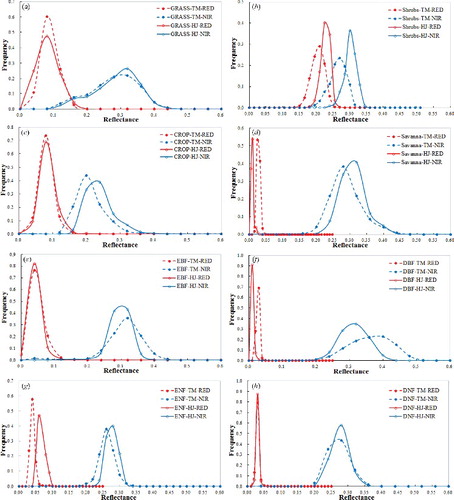
Figure 6. LAI comparison between HJ-1 CCD and Landsat TM data for eight biome types.

Figure 5 shows the spectral reflectance frequencies in the red and NIR channels for the HJ-1 CCD and Landsat TM data for different biome types. Although small differences in the peaks and tails of the histograms can be seen, the reflectance frequency distributions of the red spectral bands from the two sensors are identical to each other for most of the biomes, except for the peak frequency in the histograms of savanna and DBF, and some slight overestimation over shrubs and ENF, which exhibit a difference of ≤0.04. The reflectance frequency differences in the histograms of the NIR bands of the two sensors are ≤0.04, except for shrubs and savanna, where they are ≤0.08. These reflectance differences might be caused by the following: (1) subtle sun/view geometry differences between the HJ-1 CCD and Landsat TM satellites; (2) spectral response differences, especially in NIR band; and (3) spatial response differences. However, the differences are small and are therefore acceptable for further retrieval.

Figure 6 shows comparative histograms for the HJ-1-derived LAI and Landsat-derived LAI for different biome types. The frequency profiles show a consistent range in values between HJ-1 LAI and Landsat LAI data for EBF, and for herbaceous biomes such as grass, shrubs and crops. Differences between the peaks and tails of the LAI histograms for the two sensors are exhibited for DNF and ENF, which belong to forest classes; even here, differences are ༜1.0.

In densely vegetated areas, such as in the majority of DBF and DNF pixels, the surface spectral reflectance of HJ-1 and Landsat red bands are prone to trend toward saturation, and the surface spectral reflectance of NIR bands indicates vegetation canopy change. Since the LAI is retrieved from sets of spectral reflectances, the saturation issue leads to inconsistencies between HJ-1 and Landsat TM data retrieval. As evident for DNF in Figures 5 and 6, the NIR reflectance values for HJ-1 are higher than those of Landsat TM, probably accounting for the inconsistencies between HJ-1 and Landsat LAI values. In addition, the two DNF and ENF sites are located on the margins of northeastern China; with their differing terrains and mean altitudes above sea level of ∼1400 m, rugged topography may also account for the aforementioned inconsistencies. Inconsistencies in the DBF HJ-1 LAI and Landsat LAI data are much greater than for other biomes, but the difference is still ≤1.5, and is most likely caused by the saturated red reflectance and higher NIR reflectance values of the HJ-1 data. On the whole, most differences are acceptable and statistically insignificant, demonstrating the potential usage of the retrieval algorithm for HJ-1 satellite data.

4.2. HJ-1 LAI validation using in-situ measurements

The validation of the all-China HJ-1 LAI using ground measurements represents a highly complex task. We therefore took the Bashang Grassland and Taihe region only and attempted to cross-validate the HJ-1 LAI data using a MODIS LAI product and ground-measured LAI values.

In Figure 7, (1(1) $L=DN/Gain+Offset$(1) a) and (2(2) $L =\mathrm{ }(LMAX-LMIN)/(QCALMAX-QCALMIN)\times \left(QCAL-QCALMIN\right)+LMIN$(2) a) show the land cover map of the Bashang Grassland and Taihe regions. The dominant species is grass in the Bashang Grassland, whereas it is forest biomes such as EBF, DBF and ENF in the Taihe region. The in-situ sample sites for ground-measured LAI investigations are marked as crosses in the land cover maps. (1(1) $L=DN/Gain+Offset$(1) b) and (2b) show the HJ-1-retrieved LAI maps of the two regions, while (1(1) $L=DN/Gain+Offset$(1) c) and (2(2) $L =\mathrm{ }(LMAX-LMIN)/(QCALMAX-QCALMIN)\times \left(QCAL-QCALMIN\right)+LMIN$(2) c) show maps of these areas constructed using MODIS LAI 1 km products. The consistency in the distribution patterns of LAI values between the HJ-1-derived LAI map and the MODIS LAI map is good, except to the extent that the range in HJ-1-derived LAI values is a little larger than in that of MODIS LAI values for the Bashang Grassland, where the maximum HJ-1 LAI value is 2.8. (1(1) $L=DN/Gain+Offset$(1) d) and (2(2) $L =\mathrm{ }(LMAX-LMIN)/(QCALMAX-QCALMIN)\times \left(QCAL-QCALMIN\right)+LMIN$(2) d) separately show the correlation between HJ-1-derived LAI/MODIS LAI and ground-measured LAI values at the sample sites in the two regions. In the Bashang Grassland, as the main biome type is grass (coverage ∼70%), LAI values are lower. The HJ-1 LAI values for sample sites range from 0.21-0.78, the MODIS LAI values are 0.30-0.70, and in-situ LAI values are 0.25-0.78. For the majority (∼72%) of the 25 sample sites in the Bashang Grassland, the error in HJ-1-retrieved LAI values relative to the measured values is ≤0.2. MODIS LAI values are relatively constant because of their 1 km spatial resolution and intensive distribution shows (Figure 7, (1(1) $L=DN/Gain+Offset$(1) a)), possibly resulting in a greater margin of error. Additionally, the MODIS LAI product used plots a LAI map using the Maximum Value Composites method (MVC), potentially leading to the apparent overestimation relative to ground-measured LAI values. The HJ-1 LAI therefore performs better here. In the Taihe region, in comparison, HJ-1 LAI values range from 0.52-5.57, MODIS LAI values are 0.30-5.10, and ground-measured LAI values are 0.40-5.29. ∼72% of the errors between HJ-1-retrieved LAI and ground-measured values for the region's 32 sample sites are≤1.0. The LAI value ranges are assumed to be related to the homogeneity of the biome types. Moreover, more than half of both the HJ-1 and MODIS LAI values are underestimated, possibly caused by the nature of the forest understory and bare soil found in this region.

Figure 7. Comparison between in-situ LAI and HJ-1 LAI values for two sample sites.

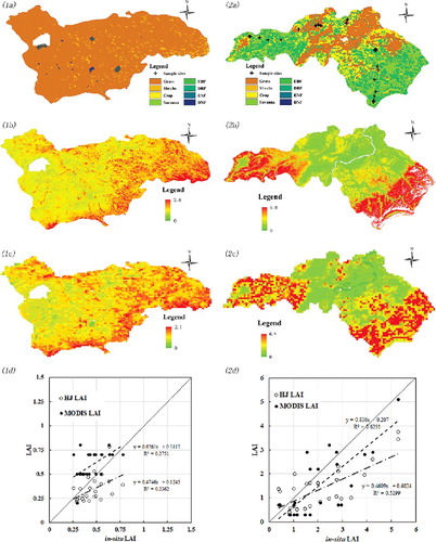
The regression equations in the scatter diagram show how the correlation between HJ-1-retrieved LAI values and ground-measured LAI values approaches the correlation between MODIS LAI values and ground-measured LAI values. Furthermore, their correlation coefficients (R) show a positive correlation in the relation between HJ-1-retrieved LAI values and ground-measured LAI values in the two study regions. Though R values are not very high, the algorithm for grass needs to be improved in future studies because of its low correlation with field LAI. However, overall, the LAI values derived from HJ-1 data indicate a promising response to ground-measured LAI values. Both cross-validation and field validation suggest the suitability of the use of the Landsat LAI algorithm in producing a HJ-1 LAI dataset for the whole of China.

4.3. Comparative analysis of HJ-1 LAI and MODIS LAI values for China

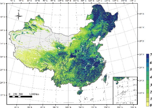
The 30m LAI map for the summer of 2012 covering the whole of China (Figure 8), and drawn by implementing the Landsat LAI retrieval algorithm, was obtained using 221 preprocessed HJ-1 CCD images. The range in LAI values for China in 2012 is within 0–7, with the mean LAI being 2.07. Moreover, the LAI is quite low in the western regions of China (e.g. in Xinjiang and Tibet) for dominant herbaceous biome types, while in eastern China, where the preponderant biome types are forests (e.g. Heilongjiang), the LAI is much higher.

Figure 8. The 30 m HJ-1 LAI map for China for the summer of 2012 using the retrieval algorithm.

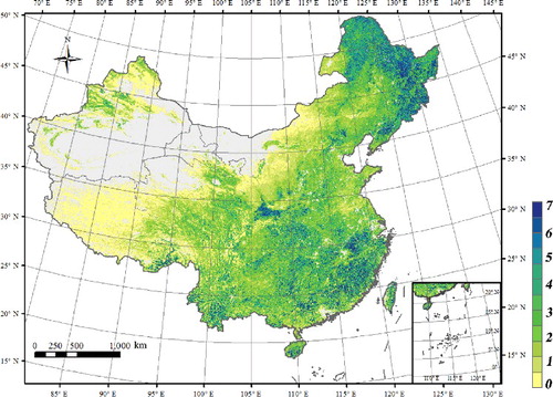
A mosaic of MODIS LAI data (Figure 9) for China for July 2012 was chosen for comparison with the 30 m HJ-1 LAI data (Figure 8). Changes in the distribution of HJ-1 LAI values were similar to those evinced by MODIS LAI data, and both LAI values were higher in northeastern and southeastern China and lower in western China.

Figure 9. MODIS LAI map for China, July 2012.

A comparison discrepancies between HJ-1 and MODIS LAI values for the eight biomes with corresponding pixels, and with the same coordinates, can be seen in Table 3. Absolute differences < 1e⁻¹⁴ for most biomes account for > 98.27% of all pixels for each same biome in China, except for grass, where 83.72% of the coverage shows an absolute difference of < 1e⁻¹⁴, and 91.35% an absolute difference of < 0.5. The mean value of the grass HJ-1 LAI is 0.22; values range from 0.03 to 6.89, and are concentrated at 0.11-1.40. As proposed in Section 4.2, these results may be affected by the bare soil. Although the HJ-1 pixel is classified as grass, it is a mixed pixel, and sensor-measured BRF can integrate the signals from pure observational components in the pixel like grass, bare soil, urban landscapes et al.

Table 3. Frequency distribution of differences between the HJ-1 LAI and MODIS LAI maps for China for eight different biome types.

△LAI	Grass	Shrubs	Crops	Savanna	EBF	DBF	ENF	DNF
[–7.0, –1.0e^−14]	9.53%	0.12%	1.03%	0.84%	0.74%	1.12%	0.45%	0.09%
(–1.0e^−14, 1.0e^−14)	83.72%	99.58%	98.48%	98.27%	98.08%	97.58%	98.88%	99.84%
[1.0e^−14, 7.0]	6.75%	0.30%	0.48%	0.89%	1.18%	1.30%	0.67%	0.07%

$\Delta LAI$is the difference in value between HJ-1 and MODIS LAI reached by subtracting MODIS LAI values from HJ-1 LAI ones.

Through analysing the frequency distributions of the LAI values of each biome type, the biomes with HJ-1 LAI frequency values somewhat higher than MODIS LAI frequency values are shrubs, EBF, DBF and ENF, while the biomes with HJ-1 LAI frequency values a little lower than MODIS LAI frequency values are grass and crops. All differences are ≤ 0.55% except grass is 2.78%. The HJ-1 LAI map for the whole of China shows an acceptable margin of error when cross-validated with MODIS LAI products.

4.4. Application of the 30 m HJ-1 LAI map

We aimed to evaluate the burned area extraction capabilities of 30 m HJ-1 LAI data. Looking at the historical background of forest fires that occurred in 2012, we selected a forest fire which occurred in Yimen County, Yunnan Province on March 18, 2012 as our test case.

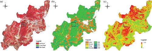
In order to sketch the burned area, images were observed and analyzed (Figure 10). In Figure 10, (a) is a HJ-1 reflectance image taken after the fire had been extinguished, (b) is a land cover map of Yimen County, and (c) is the HJ-1 LAI map of Yimen County extracted from the 30 m HJ-1 LAI map of China for the summer of 2012 (Figure 8). Because vegetation is reduced in bulk after a forest fire, LAI values are lower in the burned area than those in the unburned area (shown as the green pixels in Figure 10(c)). The black block in the images is the vague scope where LAI values are obviously lower; the surrounding pixels with low LAI values show areas covered with grass species or other non-vegetation biome types (Figure 10(b)). The abnormal region visible within the black block can also be observed in the post-fire HJ-1 reflectance image.

Figure 10. (a) The 30 m HJ-1 reflectance image, (b) land cover map and (c) HJ-1 LAI map of Yimen County.

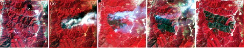
The forest fire occurred in Yimen County, Yunnan Province on the evening of 18 March 2012. The fire was brought under control by the evening of 20 March 2012. The forest fire covered an area of 120 ha during the two days over which it burnt. As shown in Figure 11, the sequential changes in the forest fire, based on the five selected HJ-1 CCD images, tally with the placement of the black block shown in Figure 10. In Figure 11, (a) shows the initial state of the fire-affected zone before the forest fire, at 03:42 hrs on 17 March 2012. In image (b), obtained at 03:42 hrs on 19 March 2012, the presence of smoke indicates that the fire had started. In image (c), obtained at 03:22 hrs on 20 March 2012, the fire had expanded. By the morning of 21 March 2012 (image (d)), the fire had been controlled and the smoke had thinned. Image (e) shows the post-fire area, on 1 May 2012.

Figure 11. Sequential HJ-1 images of the burned area caused by a forest fire in Yimen County in March, 2012.

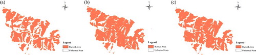
The value of M was obtained using HJ-1 reflectance data from before and after the forest fire (Figures 11(a) and 11(e)). The burned area was extracted as shown in Figure 12(a). Based on this, the value of M for the LAI in this area was 1.274, meaning that HJ-1 LAI data could help map the burned area more accurately, with a clearer discrimination between the burned and unburned areas: HJ-1 LAI data therefore, by extension, have the capacity to facilitate and enhance the accurate extraction of any burned area. This site's burned area based purely on HJ-1 reflectance data is shown in Figure 12(b), while the burned area based on HJ-1 reflectance data and HJ-1 LAI data is shown in Figure 12(c). A confusion matrix was constructed to compare the two burned area delineations, and evaluate the precision of the two results. When HJ-1 LAI data were added to the initial data, the Kappa coefficient improved from 0.8619 to 0.8628, and the overall accuracy increased from 96.17% to 96.26%. Therefore, 30 m HJ-1 LAI data have the potential to help recognize and extract the burned area more accurately, allowing a potentially more dynamic monitoring of forest fires.

Figure 12. The mapping of the post-fire burned area based on HJ-1 reflectance and LAI data.

5. Summary

A 30-m resolution HJ-1 LAI product has been proven useful for vegetation monitoring, and conducive to natural disaster mapping. In our study, we verified the consistency of the surface spectral reflectance of the two red and NIR bands between HJ-1 CCD and Landsat TM sensors over eight biomes classified by the MODIS LAI/PAR biome classification scheme, and the reflectance frequency differences were ≤ 0.04 for most biome types. The corresponding biome LAI identities were investigated and our comparisons showed a satisfactory agreement for a majority of biome types. These preliminary investigations reveal that the mature biome-specific and LUT-based Landsat-LAI algorithm is applicable to HJ-1 LAI data retrieval. The saturation issue which caused the inconsistencies in DBF HJ-1 LAI values cannot be overridden by the algorithm. In addition, field and cross-validation of the Bashang Grassland and the Taihe region were conducted to verify the feasibility of applying this algorithm. The errors relative to ground-measured LAI values were tolerable for the majority (∼72%) of the sample sites in both two regions. The MODIS LAI was overestimated relative to ground-measured LAI values for the grass biome due to its method of composition. Although the HJ-1 LAI performed better, the algorithm still needs to be improved for the grass biome type, owing to its low correlation coefficient with ground-measured data.

Owing to the higher spatial and temporal resolution of the HJ-1 LAI product, the accuracy of the sequential mapping of the burned area at a forest fire site in Yimen County in 2012 increased modestly, suggesting that use of this product might help monitor forest fires and allow decisions taken about post-fire reconstruction to be more effective. HJ-1 LAI data might therefore be more generally applicable to the development of a global LAI product with a higher spatial and temporal resolution.

Acknowledgments

The authors acknowledge all the teachers and students who have contributed to retrieving the 2012 China HJ-1 LAI map. We are grateful to the Academy of Forest Inventory and Planning, State Forestry Administration, the China Centre for Resources Satellite Data and Application and NASA, for providing the data for our research.

Disclosure statement

No potential conflict of interest was reported by the authors.

Additional information

Funding

This work was supported by Special Fund for the Ecological Assessment of the Three Gorges Project [grant number 0001792015CB5005]; Special Fund for Forest Scientific Research in the Public Welfare [grant number 201504323]; National High Technology Research and Development Programme of China (863 Program) [grant number 2013AA12A302].

References

- Baret F, Hagolle O, Geiger B, Bicheron P, Miras B, Huc M, Berthelot B, Niño F, Weiss M, Samain O. 2007. LAI, fAPAR and fCover CYCLOPES global products derived from VEGETATION: Part 1: Principles of the algorithm. Remote Sens Environ. 110:275–286.
- Chen JM, Black T. 1992. Defining leaf area index for non-flat leaves. Plant Cell Environ. 15:421–429.
- Chen JM, Pavlic G, Brown L, Cihlar J, Leblanc S, White H, Hall R, Peddle D, King D, Trofymow J. 2002. Derivation and validation of Canada-wide coarse-resolution leaf area index maps using high-resolution satellite imagery and ground measurements. Remote Sens Environ. 80:165–184.
- Chen W, Cao C, He Q, Guo H, Zhang H, Li R, Zheng S, Xu M, Gao M, Zhao J. 2010. Quantitative estimation of the shrub canopy LAI from atmosphere-corrected HJ-1 CCD data in Mu Us Sandland. Sci China Earth Sci. 53:26–33.
- Chen W, Moriya K, Sakai T, Koyama L, Cao C. 2016. Mapping a burned forest area from Landsat TM data by multiple methods. Geomat Nat Hazards Risk. 7:384–402.
- Chuvieco E, Englefield P, Trishchenko AP, Luo Y. 2008. Generation of long time series of burn area maps of the boreal forest from NOAA-AVHRR composite data. Remote Sens Environ. 112:2381–2396.
- Chuvieco E, Martin MP, Palacios A. 2002. Assessment of different spectral indices in the red-near-infrared spectral domain for burned land discrimination. Int J Remote Sen. 23:5103–5110.
- Colombo R, Bellingeri D, Fasolini D, Marino CM. 2003. Retrieval of leaf area index in different vegetation types using high resolution satellite data. Remote Sens Environ. 86:120–131.
- Cortes C, Vapnik V. 1995. Support-vector networks. Mach Learn. 20:273–297.
- Duchemin B, Hadria R, Erraki S, Boulet G, Maisongrande P, Chehbouni A, Escadafal R, Ezzahar J, Hoedjes J, Kharrou M. 2006. Monitoring wheat phenology and irrigation in Central Morocco: on the use of relationships between evapotranspiration, crops coefficients, leaf area index and remotely-sensed vegetation indices. Agric Water Manage. 79:1–27.
- Friedl MA, Sulla-Menashe D, Tan B, Schneider A, Ramankutty N, Sibley A, Huang X. 2010. MODIS Collection 5 global land cover: algorithm refinements and characterization of new datasets. Remote Sens Environ. 114:168–182.
- Ganguly S, Nemani RR, Knyazikhin Y, Wang W, Hashimoto H, Votava P, Michaelis A, Milesi C, Dungan JL, Melton FS. 2010. A physically based approach in retrieving vegetation Leaf Area Index from Landsat surface reflectance data. Proceedings of the Hyperspectral Image and Signal Processing: Evolution in Remote Sensing (WHISPERS), 2010 2nd Workshop on; IEEE.
- Ganguly S, Nemani RR, Zhang G, Hashimoto H, Milesi C, Michaelis A, Wang W, Votava P, Samanta A, Melton F. 2012. Generating global leaf area index from Landsat: algorithm formulation and demonstration. Remote Sens Environ. 122:185–202.
- Gao F, Anderson MC, Kustas WP, Houborg R. 2014. Retrieving leaf area index from Landsat using MODIS LAI products and field measurements. IEEE Geosci Remote Sens Lett. 11:773–777.
- García MA, Alloza JA, Mayor ÁG, Bautista S, Rodríguez F. 2014. Detection and mapping of burnt areas from time series of MODIS-derived NDVI data in a Mediterranean region. Cent Eur J Geosci. 6:112–120.
- Giglio L. 2007. Characterization of the tropical diurnal fire cycle using VIRS and MODIS observations. Remote Sens Environ. 108:407–421.
- Gong P, Wang J, Yu L, Zhao Y, Zhao Y, Liang L, Niu Z, Huang X, Fu H, Liu S. 2013. Finer resolution observation and monitoring of global land cover: first mapping results with Landsat TM and ETM+ data. Int J Remote Sens. 34:2607–2654.
- Huang D, Knyazikhin Y, Wang W, Deering DW, Stenberg P, Shabanov N, Tan B, Myneni RB. 2008. Stochastic transport theory for investigating the three-dimensional canopy structure from space measurements. Remote Sens Environ.112:35–50.
- Jung Y, Kim D, Kim D, Kim M, Lee SO. 2014. Simplified flood inundation mapping based on flood elevation-discharge rating curves using satellite images in gauged watersheds. Water. 6:1280–1299
- Keller M, Palace M, Hurtt G. 2001. Biomass estimation in the Tapajos National Forest, Brazil: examination of sampling and allometric uncertainties. Forest Ecol Manage. 154:371–382.
- Liang S, Zhang X, Xiao Z, Cheng J, Liu Q. 2013a. Global land surface satellite (GLASS) products: algorithms, validation and analysis. New York (NY): Springer Science & Business Media.
- Liang S, Zhao X, Liu S, Yuan W, Cheng X, Xiao Z, Zhang X, Liu Q, Cheng J, Tang H. 2013b. A long-term global land surface satellite (GLASS) data-set for environmental studies. Int J Digit Earth. 6:5–33.
- Liu W, Wang L, Zhou Y, Wang S, Zhu J, Wang F. 2016. A comparison of forest fire burned area indices based on HJ satellite data. Nat Hazards. 81:971–980.
- Mallinis G, Koutsias N. 2012. Comparing ten classification methods for burned area mapping in a Mediterranean environment using Landsat TM satellite data. Int J Remote Sen. 33:4408–4433.
- Masek JG, Vermote EF, Saleous NE, Wolfe R, Hall FG, Huemmrich KF, Gao F, Kutler J, Lim T-K. 2006. A Landsat surface reflectance dataset for North America, 1990-2000. Geosci Remote Sens Lett, IEEE. 3:68–72.
- Mei L, Xue Y, de Leeuw G, Holzer-Popp T, Guang J, Li Y, Yang L, Xu H, Xu X, Li C. 2012. Retrieval of aerosol optical depth over land based on a time series technique using MSG/SEVIRI data. Atmos Chem Phys. 12:9167–9185.
- Mei L, Xue Y, Kokhanovsky A, von Hoyningen-Huene W, de Leeuw G, Burrows J. 2014. Retrieval of aerosol optical depth over land surfaces from AVHRR data. Atmos Meas Tech. 7:2411–2420.
- Myneni R, Hoffman S, Knyazikhin Y, Privette J, Glassy J, Tian Y, Wang Y, Song X, Zhang Y, Smith G. 2002. Global products of vegetation leaf area and fraction absorbed PAR from year one of MODIS data. Remote sens Environ. 83:214–231.
- Myneni RB, Ross J, Asrar G. 1989. A review on the theory of photon transport in leaf canopies. Agric Forest Meteorol.45:1–153.
- Pereira JM, Sá AC, Sousa AM, Silva JM, Santos TN, Carreiras JM. 1999. Spectral characterisation and discrimination of burnt areas. Remote Sensing of Large Wildfires. Springer. 123–138.
- Petropoulos GP, Kontoes C, Keramitsoglou I. 2011. Burnt area delineation from a uni-temporal perspective based on Landsat TM imagery classification using support vector machines. Int J Appl Earth Obs Geoinf. 13:70–80.
- Sellers P, Dickinson R, Randall D, Betts A, Hall F, Berry J, Collatz G, Denning A, Mooney H, Nobre C. 1997. Modeling the exchanges of energy, water, and carbon between continents and the atmosphere. Science. 275:502–509.
- Thenkabail P. 2003. Biophysical and yield information for precision farming from near-real-time and historical Landsat TM images. Int J Remote Sens. 24:2879–2904.
- Thenkabail P, Ward A, Lyon J. 1994. Landsat-5 Thematic Mapper models of soybean and corn crop characteristics. Remote Sens. 15:49–61.
- Veraverbeke S, Harris S, Hook S. 2011. Evaluating spectral indices for burned area discrimination using MODIS/ASTER (MASTER) airborne simulator data. Remote Sens Environ. 115:2702–2709.
- Vermote EF, Tanré D, Deuze JL, Herman M, Morcette J-J. 1997. Second simulation of the satellite signal in the solar spectrum, 6S: An overview. GeosciRemote Sens, IEEE Trans. 35:675–686.
- Walthall C, Dulaney W, Anderson M, Norman J, Fang H, Liang S. 2004. A comparison of empirical and neural network approaches for estimating corn and soybean leaf area index from Landsat ETM+ imagery. Remote Sens Environ. 92:465–474.
- Wang Q, Wu C, Li Q, Li J. 2010. Chinese HJ-1A/B satellites and data characteristics. Sci China Earth Sci. 53:51–57.
- Weiss M, Baret F, Garrigues S, Lacaze R. 2007. LAI and fAPAR CYCLOPES global products derived from VEGETATION. Part 2: validation and comparison with MODIS collection 4 products. Remote sens Environ. 110:317–331.
- Xing Q, Hu C. 2016. Mapping macroalgal blooms in the Yellow Sea and East China Sea using HJ-1 and Landsat data: Application of a virtual baseline reflectance height technique. Remote Sens Environ. 178:113–126.
- Yang W, Zhang S, Tang J, Bu K, Yang J, Chang L. 2013. A MODIS time series data based algorithm for mapping forest fire burned area. Chinese Geogr Sci. 23:344–352.
- Yu C, Chen L. 2015. Estimating biomass burned areas from multispectral dataset detected by multiple-satellite. Spectrosc Spect Anal. 35:739–745.
- Zammit O, Descombes X, Zerubia J. 2006. Burnt area mapping using support vector machines. Forest Ecol Manage. 234:S240.
- Zhang G, Ganguly S, Nemani RR, White MA, Milesi C, Hashimoto H, Wang W, Saatchi S, Yu Y, Myneni RB. 2014. Estimation of forest aboveground biomass in California using canopy height and leaf area index estimated from satellite data. Remote Sens Environ. 151:44–56.
- Zhang J, Gu X, Wang J, Huang W, He X, Wang H. 2010. Analysis of consistency between HJ-CCD images and TM images in monitoring rice LAI. Trans Chinese Soc Agric Eng. 26:186–193.
- Zheng G, Moskal LM. 2009. Retrieving leaf area index (LAI) using remote sensing: theories, methods and sensors. Sensors. 9:2719–2745.
- Zhu Z, Bi J, Pan Y, Ganguly S, Anav A, Xu L, Samanta A, Piao S, Nemani RR, Myneni RB. 2013. Global data sets of vegetation leaf area index (LAI) 3g and fraction of photosynthetically active radiation (FPAR) 3g derived from global inventory modeling and mapping studies (GIMMS) normalized difference vegetation index (NDVI3g) for the period 1981 to 2011. Remote Sens. 5:927–948.