Fine scale population density data and its application in risk assessment

ABSTRACT

Population density is one of the key parameters for assessing the magnitude of population exposed to risk, and the better quality data we have, the better the assessment of risk. The aim of this study is to elaborate a high-resolution spatially distributed population density grid, which estimates population at the commune scale with a reliability of over 90%. The novelty of the approach is population density estimation in a regular European grid, based on buildings vector data collected in the national topographic database. Using abductive reasoning in combination with statistics and spatial analysis, the authors extract approximate information about a population from the large-scale topographic data. Moreover, linking the obtained population data with the cadastral data – by unique building identifier – allows for regular, quick and census survey-independent updates of the population surface. A shortcoming of the approach is the issue of the possible existence of two houses per family, which leads to an overestimation of population. However, in the study area it affected only two of the total 14 communes by 7%–9%.

KEYWORDS:

• Population density
• topographic database
• flooding

1. Introduction

Information on the geographical distribution of population is of critical importance in supporting decision-making in risk assessment. Risk prevention and management for natural hazards (e.g. erosion, fires, flooding, storms and drought, earthquakes) and risks linked to human activities (e.g. technological accidents) as well as civil protection and disaster management systems need access to detailed and timely information on the geographical distribution of people. This information, due to confidentiality, privacy issues and nondisclosure requirements, is generally supplied by national census at pre-defined units, mainly administrative units or statistical divisions. The size of census spatial units depends on the number of inhabitants (e.g. 4000–8000 in the U.S.A., around 500 in Poland) and it varies significantly between the dense urban areas and forestry or agricultural areas. The census gives the fullest and the most reliable characteristics of population, however, some drawbacks of this data are well known such as the long intervals between censuses which make the data outdated, or changes in border lines of census dissemination units that make long-term population comparison difficult (Gregory et al. 2010).

An important methodological problem in combining demographic data with other data for the purpose of natural hazards risk assessment is the incompatibility of mapping units used for data analysis and visualization, known in the literature as the Modifiable Areal Unit Problem (MAUP). The MAUP is ‘a problem arising from the imposition of artificial units of spatial reporting on continuous geographical phenomena resulting in the generation of artificial spatial patterns’ (Heywood et al. 1998). Research on the estimation of population data in user-defined units dates back to the beginning of the twentieth century. The cartographer Wright (1936) popularized a method of presenting population density based upon the division of a given administrative unit into smaller areas complying with different types of geographical environments and called it, after the Russian cartographer Tian-Shansky, dasymetric mapping (Bielecka 2005). Although the technique of disaggregation of census population data was described in the 1930s, it still lacks a standardized methodology. Recent advancements in geographic information systems, as well as increased availability of vector and satellite data, have revitalized the concept of presenting population counts in user-defined units. Based on the literature review, approaches used to map population differ in:

• techniques: disaggregation or aggregation;

• mapping unit (e.g. administrative units, enumeration units, geographical units, regular grid);

• ancillary data used (e.g. topographic maps, land use/land cover vector data-sets, cadastral data, satellite images, LIDAR data, etc.);

• visualization methods (e.g. choropleth map, isolines, dasymetric map, 3D visualization).

The disaggregation (down scaling) methods, based on areal interpolation, were defined by Mennis (2003, p. 32) as ‘a geographic data transformation from source zones to target zones.’ The areal interpolation, according to Langford (2013), can be implemented as: (1(1) $D{N}_{ab}= 2*SN*FN$(1) ) basic areal interpolation – without any ancillary data necessity; (2(2) $SN = 0.006*BF+0.021, \text{with }R2=0.97$(2) ) dasymetric mapping – ancillary data indispensable; and (3) statistical modelling which intends to qualify the functional relationship between variables and areal units by extracting patterns embedded in external data-sets (Mennis 2009). By contrast, the aggregation (upscaling) methods are based on summing population counts attributed to address points or buildings (Ural et al. 2011; Zandbergen 2011; Sridharan and Qiu 2013), street blocks (Mennis and Hultgren 2006; Uesugi and Asami 2016) or cadastral parcels (Maantay et al. 2007; Maantay and Maroko 2009; Jia et al. 2014), and detailed land cover and land-use data, derived mostly from satellite image classification (Bielecka 2005; Alahmadi et al. 2013; Gaughan et al. 2013; Jia and Gaughan 2016; Dmowska and Stepinski 2017).

The availability of high-resolution satellites imagery, LIDAR and fine-scale vector geographical data with detailed attributed information allows for small-area population distribution studies, but until now the results are characterized by relatively low reliability, fluctuating around 60%–70% (Yuea et al. 2005; GEOSTAT 1A 2011; Hall et al. 2012). The obtained results could be considerably improved by using regression analysis which combines the footprint areas or building volumes to the number of people in it (Wu et al. 2008; Lu et al. 2011; Alahmadi et al. 2013, 2016; Wang et al. 2016). However, Biljecki et al. (2016), based on a multi-scale study of population estimation in the Netherlands using a 3D building model, noticed that the accuracy of the obtained results strongly depends on the level of detail of the data used, and the scale of research (level of administrative units) as well as the adopted approach. Moreover, they suggested that both models, statistical and disaggregation, are able to provide truthful and comparable results.

This paper introduces and tests a new approach for refining population distribution at high resolution by combining diverse geoinformation on buildings and statistical parameters. The goal of our study is to improve the volume-based method, by combining statistical and aggregation modelling and fusing detailed information on the buildings’ location, footprint and volume as well as their structural characteristics. The buildings’ volumetric and structural characteristics (number of storeys, building type and functions) are derived from the highly reliable Polish Topographic Database. Our approach refers to both urban and rural areas, where the population distribution is very diversified, which is considered as a further benefit. Moreover, adopting the European quadrilateral grid as a mapping unit allows the comparison of results over time and the analysis together with other geographical data.

The proposed approach is based on the abductive reasoning (inferring a case from a rule and a result) that combines inductive (bottom-up, empirical) and deductive (top-down, theoretical) principles. This high resolution and highly reliable data could be used for risk estimation and management.

The article is structured as follows. Section 2 briefly describes the methods used for population surface creation and provides a short overview of global gridded population data. Sections 3 and 4 present the high-resolution local population surface generation methodology and its experimental creation for a small city and rural area located in the western part of Poland. Section 5 demonstrates the application of the created surface in risk management, namely a flood threat, which is considered the most frequent and destructive natural hazard in Poland. Finally, conclusions are drawn in Section 6.

2. Gridded population data

The advantages of using squared grid cells instead of other reference units include: simple data comparison over time and space, stable reporting of unit size and area over time, and straightforward integration with other geo-referenced geographical data. Moreover, the hierarchical construction of grid cells allows for an undemanding data aggregation. Due to these reasons census offices in some countries produced grid-based statistics, for example Austria, Finland, Norway (GEOSTAT 1A 2011), Sweden (Tufte 1990) and Great Britain (Gregory and Ell 2005; Martin 2006). In addition, three gridded products compiled over the last decade depict the distribution of human population across the globe: Gridded World Population (GPW), Global Rural-Urban Mapping Project (GRUMPv1) and LandScan. They are briefly described in the following, and summarized in Table 1.

Table 1. Characteristic of global population data.

Abbreviations of global population data	GPW	GRUMPv1	LandScan
Name	Gridded population of the world	Global Rural-Urban Mapping Project	LandScan global population
Reference years of population estimation	1990, 2000, 2005 prediction for 2010, 2015, 2020	1990, 1995, 2000	1998, annually since 2000
Format/spatial resolution	Grid/raster 2.5 arc-minutes	Grid/raster 30 arc-seconds	Grid (ESRI*format) 30 arc-seconds
Source and ancillary data	Data from national census agencies	GPW, urban mask, settlement points, NOAA's night-time lights data	Census data, roads (VmapL0), slope NIMA's DTED, global land cover database, night-time light NGDC
Method and algorithm	Disaggregation of national census data, smooth pycnophylactic (mass-preserving) interpolation (Tobler 1979)	Disaggregation of national census data, smooth pycnophylactic (mass-preserving) interpolation (Tobler et al. 1995)	Disaggregation of national census data, ‘smart’ interpolation algorithm

* Abbreviation used in the table: ESRI – Environmental Systems Research Institute, NIMA –National Imagery and Mapping Agency, DTED – Digital Terrain Elevation Data, NGDC – National Geophysical Data Center, NOAA – National Oceanic and Atmospheric Administration.

The first data-set, available from the 2004 GPW, provides globally consistent and spatially explicit human population information in 2.5 arc-minutes grid cells (Balk and Yetman 2005). The smooth pycnophylactic interpolation algorithm, elaborated by Tobler (1979), was used to transform population data from census units to a grid. The main assumption of population modelling was based on Tobler's first law of geography (Tobler 1970), which – in the context of population modelling – can be interpreted as follows. Within a given administrative unit, the areas that border on regions with higher population densities are likely to house more people than the areas that neighbour low-population density regions (Balk et al. 2011).

The GPW database was the main source of data for the GRUMPv1. The additional data-sets used to produce world population density were: settlement point location, the approximate footprint for urban centres in each country and satellite data (Balk and Yetman 2005). Aside from high-resolution gridded population data, the GRUMPv1 provides an urban extent data-set based on NOAA's night-time lights data-set and buffered settlement centroids (where night lights are not sufficiently bright) as well as point data-sets of all urban areas with populations of greater than 1000 persons.

Finally, LandScan Global Population (LandScan) is a world-wide population database in 30 arc-second resolution, estimating ambient population at risk (Dobson et al. 2000). Each raster cell is attributed with population counts based on multi-variable dasymetric ‘smart’ interpolation algorithms similar to those recommended by Tobler et al. (1995). The algorithm uses sub-national level census counts and some ancillary data including land cover, roads, slope, urban areas, village locations and high-resolution imagery analysis. The resultant population count is an ambient or average day/night population count (Bhaduri et al. 2007).

An interesting initiative of creating spatial population data-sets for the low-income countries in Africa, Asia and South America is the WorldPop project, initiated in 2013. WorldPop integrates, in open access archives, population surfaces and other demographic data (e.g. population age-structure) elaborated by researchers within the frames of AfriPop, AsiaPop and AmeriPop projects (Gaughan et al. 2013; Tatem et al. 2013). The WorldPop gridded population data-sets, with spatial resolution equal to 100 m, portray a reliable representation of population distributions based on census data (Tatem et al. 2007), survey (Alegana et al. 2015), satellite (Linard et al. 2012; Stevens et al. 2015), social media (Linard et al. 2014), cell phone (Deville et al. 2014) and other spatial data-sets (Tatem et al. 2007). The method is based on the ‘Random Forest’ flexible, semiautomatic model to estimate population counts in a grid cell. Moreover, the data are accompanied by metadata and measures of uncertainty (Tatem and Linard 2011), which is perceived as the great advantage of WorldPop. The researchers noticed that the modelling method used in the WorldPop project produce more accurate data-sets than the methods used in the elaborating of global gridded population data products like GRUMPv1, GPW and LandScan (Linard et al. 2012; Tatem et al. 2013).

The 1 sq⋅km European population grid was introduced in 2011 (GEOSTAT 1A 2011) and amended in 2014 (EFSG 2014). The data covers 28 European Union Member States and the four EFTA (European Free Trade Association) countries. Hence, the GEOSTAT model considers differences in available resources and utilizes two methods for allocating a number of inhabitants to each square kilometre cell: aggregation or disaggregation (Moström and Wardzińska-Sharif 2016). The aggregation method (bottom-up approach) relies on aggregating geo-referenced micro data (e.g. address points, buildings, centroids of parcels) and census 2011 data-sets. Alternatively, when geo-referenced micro data are not available the disaggregation (top-down) approach was used. The disaggregation method utilizes statistical population data for the lowest administrative units in combination with supplementary spatial data (e.g. land cover/land use or European imperviousness data-set). Countries where geo-referenced address points or buildings are available only partially implemented the hybrid approach, which is aggregation and disaggregation (Dudova and Ahmedov 2013).

The main disadvantage of the existing gridded population data is their low and variable (within one data-set) reliability of population counts attributed to grid cells. Hall et al. (2008, 2012) pointed out the large differences between the described world gridded population databases as well as between the reference census and ancillary data. The European gridded population data is also imprecise. The percentage error of population estimation is between 25 for the Netherlands and more than 50 for Norway (Eurostat 2011; Nordbeck 2012). Despite the fact that the pan-European population grid is of low quality the lesson learned allowed the improvement of the population grid model and techniques and awareness of the countries’ importance of high quality geo-reference data on address points, buildings or cadastral centroids.

3. Case study of Siedleckie region

3.1. Study area and data

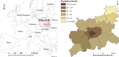
The study area consists of the city of Siedlce and, mostly rural, Siedleckie county located in Mazovia, in the western part of Poland. According to the 2013 Polish statistical data, the population distribution in the study area varies considerably from the highly populated city of Siedlce (2397 people per square kilometre) to the sparsely populated commune of Korczew (27 people/sq⋅km). This is illustrated in Figure 1, by the means of a choropleth map (classification based on manual choice). Moreover, the size of reference units of the officially available census data, representing the third level of Polish administrative division – communes – is heterogeneous, and varies from 47 to 123 km².

Figure 1. Location of the study area (a) and its population density per census track (b).

The building data layer from the Polish Database of Topographic Objects (BDOT10k) was used as the ancillary data. It is a country wide vector database with a thematic scope and a level of detail corresponding to civilian topographic maps at a scale of 1:10,000. The BDOT10k buildings are represented geometrically by polygons and they are described by 25 attributes. Several of them, namely building footprint, building type, its functions and number of storeys, are crucial for this research. The accuracy of the BDOT10k building location is very high; the average displacement between ground survey measurements and the building footprint coordinates, in the topographic database is 2 m (Bielecka 2015). A summary of an overview description of census and auxiliary data used is given in Table 2. Data are provided by Central Statistical Office of Poland.

Table 2. The study area and auxiliary data overview.

Items	Building data from BDOT10k
	City of Siedlce	Siedleckie county
Available year of data	2013
Coordinate reference system	1992
Total number of buildings	14,904	75,559
	Census data for 2013
Population	76,585	81,685
Total area in square kilometres	31.95	1603.27
Population density per square kilometre	2397	51
Average size of private households (the mean average number of people (adults and children) per household)*	2.53	3.00

*OECD definition (OECD 2016).

The study of the building vector layer of the existent topographic data, followed by the field study of the test area, allowed for some gains in information about the types of buildings intended for permanent human habitation. Following the building typology as defined in the Database of Topographic Objects, we distinguished the following three residential building types depending on dwelling number:

• single-family building, also called single-family detached home or separate house – a single dwelling unit inhabited by a family or small group sharing facilities such as a kitchen;

• two-flat residence, sometimes referred to as a two-flat or duplex or semi-detached building – a double dwelling unit inhabited by two families, or building consisting of two separate houses typically interconnected side by side;

• a multi-family residential dwelling, also called an apartment building – a building with multiple apartments.

Within the study area, residential buildings constitute 55.5% of all buildings in the city of Siedlce and 36.3% in Siedleckie county, while the total area occupied by these residential houses equals 6.6% in the city, and 0.9% in the county. Moreover, the multi-family houses predominate in the city (87.3%), while single-family houses (99.7%) predominate in the county (see Table 3).

Table 3. Residential houses in the study area by type.

Residential buildings types	Siedlce city	Siedleckie county
Total number of residential houses	8277	27,469
Single-family house	1049	27,392
Two-flat residence	2	74
Apartment building	7226	3

All non-residential buildings, as well as non-residential levels of the mixed-use buildings (that constitute less than 0.2% of total buildings number), were excluded from the subsequent analysis. The study did not include people living in student hostels, boarding schools, nursing homes, etc., and those living in places not intended for residential purposes, but which for various reasons are inhabited (e.g. garden houses).

3.2. Methods

The study aimed at the provision of a high-resolution population density grid, which estimates population density with a reliability of over 90%. The main advantage of grid-based models of population distribution are as follows: (1(1) $D{N}_{ab}= 2*SN*FN$(1) ) population density data is represented as a continuous surface and (2(2) $SN = 0.006*BF+0.021, \text{with }R2=0.97$(2) ) it is unconstrained by any of the irregular partitioning into arbitrary areal units, i.e. administrative or census enumeration and thus it is not subject to the MAUP and other areal unit-derived problems (Langford 2013; Mennis 2003).

The main assumptions in the presented model are as follows: population density is proportional to the total number of dwellings in each building and housing density, defined after Bender (1981) as the number of dwellings per unit of land. This imposes the second assumption stating that population surface represents population of place of residence at night time, i.e. the number of people staying at home at night. The third assumption is that population total for the study area (county – the second level of administrative unit) should be preserved, while in the commune (the third, lowest level of administrative division) the differences between expected (given by the Central Statistical Office) and computed population are minimized.

The buildings’ volumetric and structural characteristics (i.e. building location, footprint, building type, its functions and number of storeys) were extracted from the Polish Database of Topographic Objects, while the required dwelling number was estimated using abductive reasoning in combination with statistical analysis. In particular, a statistical relationship between the apartment building footprint area and the number of its dwellings was established by means of regression analysis based on a sample of randomly distributed field data.

The estimated total number of building dwellings was then multiplied by the average private household size provided by the Central Statistical Office in Poland depending on the commune level of urbanization (see Table 2) to arrive at an initial building population estimate. By summing up these initial figures of each building located within a chosen commune, an initial commune total population approximation was accomplished. The sum of the squares of the residuals, representing the differences between the expected census origin commune population and the approximate one, was then minimized by modifying the average size of private households at the commune level. It resulted in obtaining a refined household average size for each of the communes and, subsequently, it altered the inhabitant number for each residential building, i.e. a more refined building population estimate was attained.

Finally, the refined building population was related to the European geographical quadrilateral grid system. It is a hierarchical, two-dimensional grid geographically based on the ETRS89 Lambert Azimuthal Equal Area coordinate reference system (INSPIRE 2010), established as a spatial data frame for thematic information linking within the European Union. For this analysis, the 100 m resolution grid cell was chosen and the fine-scale population density raster was created. Then, the accuracy of the fine-scale population grid was verified at the commune scale. In the closing step, a choropleth map was created in order to visualize the obtained population density surface.

4. Results and discussion

4.1. Number of apartment building dwellings estimation

A study area field reconnaissance revealed the fact that each staircase is associated with two apartments on each floor (Figure 2). The ground truth data of the number of dwellings in each apartment building is unavailable, however it can be estimated on the base of the following equation(1) $D{N}_{ab}= 2*SN*FN$(1) :(1) $D{N}_{ab}= 2*SN*FN$(1) where DN_ab – estimated number of dwellings in an apartment building; SN – number of staircases in an apartment building; FN – number of floors in an apartment building.

Figure 2. Typical apartment building in the study area. Source: own archives.

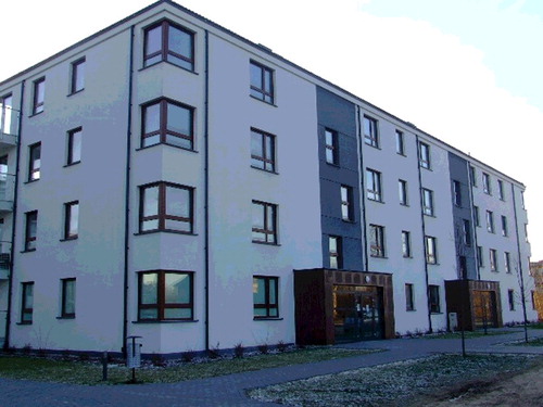
As may be noticed from the provided photograph of a standard apartment building in the study area (Figure 2), it is composed of several internal entrances and each entrance has only one staircase. Moreover, each floor has the same area. A sample of 310 residential buildings was used to model a statistical relationship between the number of residential building staircases and the apartment building basic footprint area. This hypothesis was positively verified through a regression analysis (Figure 3).

Figure 3. The relationship between the number of staircases and the building basic footprint.

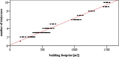
The relationship between the number of an apartment building staircases and the building footprint (area) can be modelled using a simple linear regression (2(2) $SN = 0.006*BF+0.021, \text{with }R2=0.97$(2) ):(2) $SN = 0.006*BF+0.021, \text{with }R2=0.97$(2) where SN – number of staircases in an apartment building; BF – building basic footprint (m²).

The value of coefficient of determination (R²) equals 0.97 what means that the number of staircases in one apartment building is explained in 97% by the building footprint area.

4.2. Commune population estimation

Assuming the average size of private households ($c_i$) is known, the building inhabitant's number in each of the building types follows the simple rule illustrated in Table 4.

Table 4. Number of inhabitants in a building approximation.

Building type	Number of dwellings	Number of inhabitants
Single-family house	1	$1*c_i$
Two-flat residence	2	$2*c_i$
Apartment building	DN	$DN*c_i$

The initial number of residents in each building was estimated using the official average size of private households listed in Table 2. Its initial value is equal to 3.00 or 2.53 depending on commune urbanization type.

By summing up the initial estimated numbers of building inhabitants for all buildings geographically located in a commune, the approximate commune total population was obtained. To arrive at a finer approximation (‘best fit’) of population at the commune level, the sum of the squares of the differences between the expected value, that is census origin commune population, and the initial commune population estimation was minimized by the manipulation of the average size of private households at the commune level. The final c_i coefficient values are: 2.65 for the city of Siedlce; 2.3 for the rural commune Korczew; 2.68 for municipalities of Mordy and Przesmyki and 3.0 for the rest of the rural communes.

4.3. Fine-scale population density surface creation and its accuracy verification

The estimated number of building dwellings was then multiplied by the tuned average private households for each building located in a particular grid cell, and summed up to arrive at the cell population value. Here, the authors refer to the location of the building as to the building centroid position.

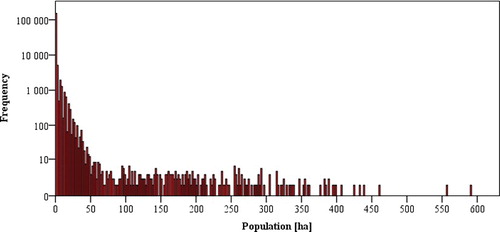
The final population density attributed to 1 ha grid varies from 0 to 635 as can be seen from histogram (Figure 4).

Figure 4. Histogram of cell grid population density (number of people per 1 ha).

In order to verify the accuracy of the resulting population surface, a comparative analysis was performed. The limited reference data availability allowed only for analysis on the third level of the Polish administrative division (i.e. at the commune scale). The obtained root mean square error of population estimation equals to 89 people, and mean absolute deviation of 3.9 (Table 5).

Table 5. Accuracy verification – error statistics.

Descriptive statistic	People per commune
Mean	–22.14
Median	50.50
Standard deviation	320.04
Range	1053.76
Min	–568.10
Max	485.66
Error statistics
Level of significance (95%)	193.40
MAD	3.94
RMSE	88.76

The minimal value of –586.10 (see Table 5), relating to the number of people in the Siedlce commune, is the highest overestimation of the population. It is, however, only 3.3% of the population in the commune (see Figure 5). The maximum value of 485.66 people is the greatest underestimation (the Skorzec commune) and represents 6.3% of the total population in the commune.

Figure 5. The differences in per cent in population counts (MAPE error) by commune (choropleth map, equal interval classification method).

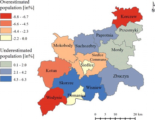
The difference in per cents in population counts (MAPE error), shown on Figure 5, varies from −6.3 to +8.85, when comparing population by commune given by the Central Statistical Office to the total population derived from the interpreted population surface. The population in the two communes, namely Skorzec and Wisniew, was underestimated by 4%–6%. The underestimation could be a result of errors in the topographic data, especially with omission of some apartment buildings, misclassification of a building type (e.g. residential, office or other), or because of an incorrect value of the number of storeys. It is worth mentioning that according to the technical specifications of the Polish Database of Topographic Objects (BDOT10k), 2% of buildings omission is acceptable (MIAA 2011).

For the other two peripheral communes, mainly tourist and recreational areas, the population approximation was overestimated around 7%–9%. This is attributed to the existence of summer houses, i.e. used only temporarily as a house, that should not be included in the model. However, they are not possible to identify and subsequently exclude from further calculations, based only on the national topographic data. In the city of Siedlce overestimation could be related to apartments not inhabited yet, e.g. not sold by the developer or intended for rental but currently vacant.

4.4. Cartographic visualization

The obtained population surface represents detailed high-resolution population density data. It is a next research challenge to visualize it in the most efficient and easily readable way to take advantage of the spatial distribution of population density. The authors believe that the form of choropleth map proposed below (Figure 6) possesses these qualities, however, they are more evident if the map is displayed in the appropriate scale depending on user experience and cognition capacities (e.g. as one of the zoomable layers in a geoportal).

Figure 6. Population density map (classes chosen using natural breaks).

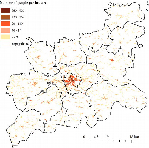
The population density choropleth map (Figure 6) allows for a quick visual assessment of the population data spatial distribution (Calka et al. 2016). The prevalence of the unpopulated areas is easily perceived. And indeed, they constitute 92.5% of the total study area. The very low populated regions, i.e. 2–19 people per hectare, correspond to rural areas with dispersed settlement, where 46% of the population live. By contrast, only 5% of the total population lives in the most densely populated regions, denominated by 360–635 habitants per hectare, covering only 0.01% of the study area. Those most populated regions correspond to town areas and some county villages areas (most populous ones).

5. Application of fine-scale population density data in flood risk exposure

Poland, a country located in central-eastern Europe, suffers few natural hazards except for an occasional flooding, with a prevalence of early spring floods. This fact is emphasized by researchers (Zolina 2012; Kundzewicz 2014; Kundzewicz et al. 2016), and international and national bodies involved in natural hazards (CEC 2007; IRFC 2010; CIA 2016). In the last 40–50 years, the annual number of heavy floods and damages caused by inundation have increased considerably (Kundzewicz 2014; Anderson 2007). However, an awareness and preparedness for such hazards have become a serious concern following the dramatic floods in Poland (and neighbouring countries, i.e. Germany and the Czech Republic) in 1997 and 2010. During the last 20 years, several country wide initiatives have come into existence, amongst which the IT system of the Country's Protection Against Extreme Hazards (ISOK) is one of the major ones. Some of the prevention products of ISOK are recently elaborated flood hazard maps and flood risk maps (Nowicki 2007; ISOK 2015), and the vector data of areas at flood risk are available to download by the public (e.g. using the spatial web services).

Sharing data on flood risk along with information about the number of people exposed to danger enables a wide and open access for all citizens (Fiedukowicz et al. 2012) and it facilitates people protection measures both in crisis situations and risk mitigation. Regardless the size and character of the hazard, people are always first and foremost affected locally, that is, where they live and conduct their daily activities (Freire 2010). Unfortunately, the ISOK system does not collect any data on population distribution. The described high-resolution population distribution surface fills this gap.

Usefulness of the data is demonstrated in an example of flood hazard in the study area crossed by two main rivers, the Bug and the Liwiec. The vector data representing areas at flood risk from the rivers, identified by ISOK, can be overlaid and intersected with the final population density grid to derive the number of people exposed to flood risk. The areas marked with the 1% probability of the Bug or Liwiec flooding (i.e. once in 100 years) are inhabited by 1782 people which accounts for 1.14% of the study area population (Figure 7). Residents of eight villages of the Korczew commune live in the highest risk area, in particular those whose houses are on the Bug River floodplain. Those in danger (925 people) constitute 30.04% of Korczew commune residents. In case of flooding 24 coaches and 78 lifeboats will be needed, assuming that one boat can carry 12–15 people. Altogether the number of buildings which may be destroyed by flooding is 949, out of which there are 402 residential houses and 547 other buildings. In this area there is also a primary school with 200 pupils. It is the most vulnerable people needing some form of rapid extraction.

Figure 7. Visualization of the areas threatened by Bug and Liwiec floods in the study area.

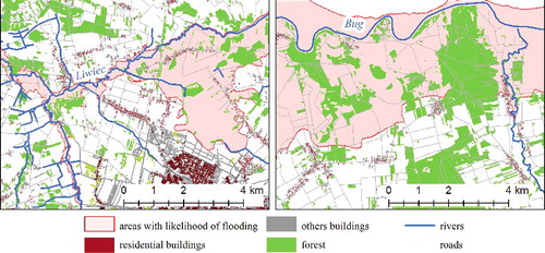
The Liwiec River in the Siedlce commune does not pose as much threat as the Bug River (Nowicki 2007). Out of 17,496 residents, 652 people live in the risk area, which is 3.73% of the total population of the commune. Due to flooding 492 buildings (3.81% of all buildings in the commune) may be damaged, including 217 residential houses (1.68% of all houses in the commune) and 275 other buildings (2.13% in the commune).

It is also worth mentioning that only 4803 people live within 100 m of all the rivers in the study area, accounting for 3.1% of the population, while up to 13,710 (8.4%) inhabitants live within 300 m of the rivers. Although the modelled population surfaces represent maximum expected night-time densities, the number of people at risk is probably unchanged from night time to daytime due to agricultural character of the most affected areas.

So far, the number of residences affected by flooding is only roughly estimated, based on interviews with local people and total number of people in the commune.

6. Conclusions

Population grid represents both population distribution and density, and can be easily combined with hazard maps for exposure assessment or modelling. The authors’ method of producing a population density surface is a bottom-up approach based on the computation of the number of people in each cell by an estimation of the number of inhabitants in every dwelling spatially joined with grid cells. The fine resolution local population surface is a gridded data product that renders population data at the scale and the extent required to demonstrate the spatial relationship of human population and the environment on a local scale. The presented grid creation method proved to be successful for medium-small regions characterized by uneven population distribution with large differences between the highest and the lowest population densities. The reliability of the fine-scale population density grid in comparison with census counts is over 90%. Moreover, the use of the fine-scale population density grid, where people are assigned to the cell where they actually live, avoids the MAUP issue.

Unlike other studies, population estimation based on the number of dwellings by type and function of building allows for the exclusion of non-residential parts of mixed-use buildings. Another advantage of the elaborated method is the possibility of quick and census survey-independent data updating. Linking the population surface with the cadastral data – by unique building identifier – allows for regular updates.

The proposed model is scalable and could be applied and customized for other rural–urban area in Poland and other European countries, ultimately benefiting disaster risk assessment and mitigation. However, usability of the fine-scale population density surface method requires an access to high-resolution detailed data on buildings, in particular their location, number of storeys as well as their types, including residential buildings’ ones. This kind of information is usually stored in fine-scale topographic data. Such a detailed database is not available in each country. In some countries (e.g. France, Germany, the Netherlands), the stored data on buildings’ height can be used to estimate the number of storeys (Dukaczewski 2013). In such a case, the expected results could be a little less accurate, which is pointed out by Biliecki et al. (2016). The other shortcomings of the presented approach are as follows: the issue of two houses per family, i.e. the permanent and the summer one, and the issue of uninhabited dwellings. Such occurrences lead to an overestimation of number of inhabitants. However, in the tested area it affected only two out of 14 communes by 7%–9%.

It should be emphasized that since 2010 the European Commission, together with Member States, has been working on spatial data (including data on buildings) harmonization within the frame of INSPIRE - Infrastructure for Spatial Information in the European Community. The application schema of buildings data includes information on the number of storeys and the number of dwellings (INSPIRE 2012). Such information allows for more accurate estimation of number of people not only at the grid cell level, but also at the building feature level of detail. However, according to the schedule (INSPIRE Road Map 2015) the data will be available after 2021.

The authors plan to update the model based on its validation in other test areas. The further work will include spatio-temporal distribution of population, e.g. at day and night time. Moreover, the authors plan to share this data in the geoportal of Siedleckie region and cooperate with the local authorities in order to use the population density surface in local applications.

Acknowledgments

The authors thank the reviewers for their helpful and constructive comments that greatly contributed to improving the final version of the paper. This work was supported by the Military University of Technology, Faculty of Civil Engineering and Geodesy under statutory research no. PBS/933/2016.

Disclosure statement

No potential conflict of interest was reported by the authors.

Additional information

Funding

Military University of Technology, Faculty of Civil Engineering and Geodesy [grant number PBS/933/2016].

References

- Alahmadi M, Atkinson PM, Martin DA. 2013. Estimating the spatial distribution of the population of Riyadh, Saudi Arabia using remotely sensed built land cover and height data. Comput Environ Urban Syst. 41:167–176.
- Alahmadi M, Atkinson PM, Martin DA. 2016. Comparison of small-area population estimation techniques using built-area and height data, Riyadh, Saudi Arabia. IEEE J Sel Top Appl Earth Obs Remote Sen. 9(5):1959–1969.
- Alegana VA, Atkinson PM, Pezzulo C, Sorichetta A, Weiss D, Bird T, Erbach-Schoenberg E, Tatem AJ. 2015. Fine resolution mapping of population age-structures for health and development applications. J R Soc Interface. 12:20150073.
- Anderson J. 2007. Climate change-induced water stress and its impact on natural and managed ecosystems. Report European Parliament IP/A/CLIM/ST/2007.06. Brussels: European Parliament Temporary Committee on Climate Change.
- Balk DL, Deichman U, Yetman G, Pozzi F, Hay SI, Nelson A. 2011. Determining global population distribution: methods, applications, data. Adv Parasitol. 62:119–156. doi:10.1016/S0065-308X(05)62004-0
- Balk D, Yetman G. 2005. The global distribution of population: evaluating the gains in resolution refinement. Center for International Earth Science Information Network (CIESIN), Columbia University. [updated 2016 Nov 10]. http://beta.sedac.ciesin.columbia.edu/gpw/docs/gpw3_documentation_final.pdf.
- Bender B. 1981. Urban housing density and the price of housing services. J Urban Econ. 9(1):80–84. doi:https://doi.org/10.1016/0094-1190(81)90049-8
- Bielecka E. 2005. A dasymetric population density map of Poland. In Proceedings of the International Cartographic Conference; July 9--16; La Coruna. Spain: ICC/ICA; [cited 2016 May 31]. http://icaci.org/files/documents/ICC_proceedings/ICC2005/htm/pdf/oral/TEMA5/Session%209/ELZBIETA%20BIELECKA.pdf
- Bielecka E. 2015. Geographical data sets fitness of use evaluation. Geodetski Vestnik. 59(2):335–348. doi:10.15292/geodetski-vestnik.2015.02.335-348
- Biljecki F, Ohori KA, Ledoux H, Peters R, Stoter J. 2016. Population estimation using a 3D city model: a multiscale country-wide study in the Netherlands. PLoS One. 11(6):e0156808. [updated 2016 Jun 2]. https://doi.org/10.1371/journal.pone.0156808
- Bhaduri B, Bright E, Coleman P, Urban M. 2007. LandScan USA: a high resolution geospatial and temporal modeling approach for population distribution and dynamics. Geo J. 69:103–117.
- Calka B, Bielecka E, Zdunkiewicz K. 2016. Redistribution population data across a regular spatial grid according to buildings characteristics. Geod Cartography. 65(2):149–162. doi:https://doi.org/10.1515/geocart-2016-0011
- [CEC] Commission of European Communities. 2007. Directive 2007/60/EC of the European parliament and of the council on the assessment and management of floods. OJ L 288, 6.11.2007, p. 27–34.
- [CIA] Central Intelligence Agency[Internet]. 2016. The World Factbook: Poland 2013--14. Washington (DC): Central Intelligence Agency; [cited 2016 Oct Jun 8]. www.cia.gov/library/publications/the-world-factbook/fields/2021.html
- Deville P, Linard C, Martine S, Gilbert M, Stevens FR, Gaughan AE, Blondel VD, Tatem AJ. 2014. Dynamic population mapping using mobile phone data. Proc Natl Acad Sci. 111(45):15888–15893. doi:10.1073/pnas.1408439111
- Dmowska A, Stepinski TF. 2017. A high resolution population grid for the conterminous United States: the 2010 edition. Comput Environ Urban Syst. 61:13–23.
- Dobson JE, Bright EA, Coleman PR, Durfee RC, Worley BA. 2000. LandScan: a global population database for estimating populations at risk. Photogramm Eng Remote Sens. 66:849–857.
- Dudova I, Ahmedov A. 2013. Prototype of Bulgarian population grid. Hybrid solution in producing. Paper presented at: European Forum for Geostatistics, 23–25 October, Sofia, Bulgaria: [cited 2016 Oct Jun 8]. http://www.efgs.info/wp-content/uploads/geostat/1b/GEOSTAT1B-Appendix8-WP1B-Presentation-DUDOVA_AHMEDOV.pdf
- Dukaczewski D. 2013. Comparison of BDOT10k and other European topographic data bases [Porownanie BDOT10k z europejskimi bazami danych topograficznych]. Rola bazy danych obiektow topofraficznych w tworzeniu infrastruktury informacji przestrzennej w Polsce. Warsaw: GUGiK. Polish.
- [EFSG] European Forum for Geography and Statistics. 2014. GEOSTAT 1B. Final management report – February 2014. Oslo: European Statistical System; [cited 2016 Oct Jun 15]. http://www.efgs.info/geostat/1B/
- Eurostat [Internet]. 2011. Population grids. [updated 2016 Jun 15]. http://ec.europa.eu/eurostat/statistics-explained/index.php/Population_grids#cite_note-3.
- Fiedukowicz A, Gasiorowski J, Kowalski P, Olszewski R, Pillich-Kolipinska A. 2012. The statistical geoportal and the “cartographic added value” – creation of the spatial knowledge infrastructure. Geod Cartography. 61:47–70.
- Freire S. 2010. Modeling of spatio-temporal distribution of urban population at high-resolution – value for risk assessment and emergency management. In: Konecny M, Zlatanova S, Bandrova TL, editors. Geographic information and cartography for risk and crisis management. Lecture notes in geoinformation and cartography. Berlin: Springer; p. 53–67.
- Gaughan AE, Stevens FR, Linard C, Jia P, Tatem AJ. 2013. High resolution population distribution maps for Southeast Asia in 2010 and 2015. PLoS One. 8(2):e55882. doi:10.1371/journal.pone.0055882
- GEOSTAT 1A. 2011. ESSnet project GEOSTAT — Representing census data in a European population grid final report for A 2010-2011. 1. Final Report for A 2010–2011. Oslo: European Statistical System.
- Gregory IN, Ell PS. 2005. Breaking the boundaries: geographical approaches to integrating 200 years of the census. R Stat Soc. 168:419–437.
- Gregory IN, Marti-Henneberg J, Tapiador FJ. 2010. Modelling long-term pan-European population change from 1870 to 2000 by using geographical information systems. J R Stat Soc. 173:31–50.
- GUS. 2014. Statistical portrait of Siedlce in the years 2005–2012. Statistical Office in Warsaw. [cited 2016 Jun 2]. http://warszawa.stat.gov.pl/publikacje-i-foldery/inne-opracowania/statystyczny-portret-siedlec-w-latach-2005-2012,20,1.html
- Hall O, Duit A, Caballero L. 2008. World poverty, environmental vulnerability and population at risk for natural hazards. J Maps. 4(Special Issue):151–160.
- Hall O, Stroh E, Paya F. 2012. From census to grids: comparing gridded population of the world with Swedish census records. Open Geogr J. 5:1–5. doi:1874-9232/12 2012
- Heywood D, Cornelius JS, Carver S. 1998. An introduction to geographical information systems. New York (NY): Addison Wesley Longman.
- INSPIRE. 2010. D2.8.I.2 INSPIRE specification on geographical grid systems – guidelines. [updated 2016 Jun 2]. http://inspire.ec.europa.eu/document-tags/data-specifications
- INSPIRE. 2012. D2.8.III.2 INSPIRE data specification on buildings – technical guidelines. http://inspire.ec.europa.eu/document-tags/data-specifications
- INSPIRE. 2012. INSPIRE Road Map [cited 2017 Jan 10]. http://inspire.ec.europa.eu/inspire-roadmap/61
- IRFC. 2010. Poland struggles to cope with heavy rain and floods, The International Federation of Red Cross and Red Crescent Societies (IFRC). [updated 2016 Jun 2]. http://www.ifrc.org/fr/nouvelles/nouvelles/europe/poland/poland-struggles-to-cope-with-heavy-rain-and-floods/
- ISOK. 2015. IT system of the country's protection against extreme hazards. [cited 2016 Oct Jun 8]. http://www.isok.gov.pl/en/
- Jia P, Gaughan AE. 2016. Dasymetric modeling: a hybrid approach using land cover and tax parcel data for mapping population in Alachua County, Florida. Appl Geogr. 66:100–108. [updated 2016 Jun 2]. https://doi.org/10.1016/j.apgeog.2015.11.006
- Jia P, Qiu Y, Gaughan AE. 2014. A fine-scale spatial population distribution on the high-resolution gridded population surface and application in Alachua County, Florida. Appl Geogr. 50:99–107. [updated 2016 Jun 2]. https://doi.org/10.1016/j.apgeog.2014.02.009
- Kundzewicz WZ. 2014. Adapting flood preparedness tools to changing flood risk conditions: the situation in Poland. Oceanologia. 56(2):385–407. doi:10.5697/oc.56-2.385
- Kundzewicz ZW, Stoffel M, Niedźwiedź T, Wyżga B. 2016. Flood risk in the Upper Vistula Basin. Germany, GeoPlanet: Earth and Planetary Sciences. [updated 2016 Jun 2]. doi:10.1007/978-3-319-41923-7
- Langford M. 2013. An evaluation of small area population estimation techniques using open access ancillary data. Geogr Anal. 45:324–344.
- Linard C, Gilbert M, Snow RW, Noor AM, Tatem AJ. 2012. Population distribution, settlement patterns and accessibility across Africa in 2010. PLoS One. 7(2):e31743. doi:10.1371/journal.pone.0031743
- Linard C, Patel N, Stevens FR, Huang Z, Gaughan AE, Tatem AJ. 2014. Use of active and passive VGI data for population distribution modelling: experience from the WorldPop project. In: Proceedings of the GIScience Workshop: Role of Volunteered Geographic Information in Advancing Science: Effective Utilization; [cited 2017 Jan 10]. http://web.ornl.gov/sci/gist/workshops/2014/
- Lu Z, Im J, Quackenbush LA. 2011. Volumetric approach to population estimation using Lidar remote sensing. Photogramm Eng Remote Sens. 77(11):1145–1156. doi:10.14358/PERS.77.11.1145
- Maantay J, Maroko A. 2009. Mapping urban risk: flood hazards, race, and environmental justice in New York. Appl Geogr. 29:111–124.
- Maantay JA, Maroko AR, Herrmann C. 2007. Mapping population distribution in the urban environment: the cadastral-based expert dasymetric system (CEDS). Cartography Geogr Info Sci. 34:77–102.
- Martin D. 2006. An assessment of surface and zonal models of population. Int J Geogr Info Syst. 10(8):973–989.
- Mennis J. 2003. Generating surface models of population using dasymetric mapping. Prof Geogr. 55:31–42.
- Mennis J. 2009. Dasymetric mapping for estimating population in small areas. Geogr Compass. 3:727–745.
- Mennis J, Hultgren T. 2006. Intelligent dasymetric mapping and its application to areal interpolation. Cartography Geogr Infor Sci. 33:179–194.
- MIAA. 2011. Regulation of the minister of internal affairs and administration of 17 November 2011 on topographic objects database and database of general geographic objects and the standard cartographic elaborations. J Laws. 279(1642):16096–16099. Polish.
- Moström J, Wardzińska-Sharif A. 2016. Spatializing statistics in the ESS. Results from the 2015 GEOSTAT 2 survey on geocoding practices in European NSIs. Sweden: Eur Forum GeogrStat; [cited 2016 May 22]. http://www.efgs.info/geostat/geostat2/
- Nordbeck O. 2012. Testing and quality assessment of pan-European population grids – based on the Norwegian experience. ESSnet project GEOSTAT 1B. WP-1A Testing and quality assessment. Stokholm (Sweden): European Forum for Geography and Statistics; [cited 2017 Jan 10]. http://www.efgs.info/wp-content/uploads/geostat/1b/GEOSTAT1B-Appendix3-Testing-and-QualityAssessment-of-PanEU-grids.pdf
- Nowicki Z. 2007. Map of areas with likelihood of flooding in Poland [Mapa obszarów zagrożonych podtopieniami w Polsce]. Warsaw, Poland: Polish Geological Institute. http://www.psh.gov.pl/plik/id,4710,v,artykul_3966.pdf.Polish.
- OECD. 2016. OECD family database. Paris, France: OECD – Social Policy Division – Directorate of Employment, Labour and Social Affairs. [cited 2017 Jan 10]. www.oecd.org/els/family/database.htm.
- Sridharan H, Qiu F. 2013. A spatially disaggregated areal interpolation model using light detection and ranging-derived building volumes. Geogr Anal. 45:238–258.
- Stevens FR, Gaughan AE, Linard C, Tatem AJ. 2015. Disaggregating census data for population mapping using random forests with remotely-sensed and ancillary data. PLoS One. 10(2):e0107042. doi:10.1371/journal.pone.0107042
- Tatem AJ, Gaughan AE, Stevens FR, Patel NN, Jia P, Pandey A, Linard C. 2013. Quantifying the effects of using detailed spatial demographic data on health metrics: a systematic analysis for the AfriPop, AsiaPop, and AmeriPop projects. Lancet North Am Ed. 381:S142. doi:https://doi.org/10.1016/S0140-6736(13)61396-3
- Tatem AJ, Linard C. 2011. Population mapping of poor countries. Nature. 474(7349):36. doi:10.1038/474036d
- Tatem AJ, Noor AM, von Hagen C, Di Gregorio A, Hay SI. 2007. High resolution population maps for low income nations: combining land cover and census in East Africa. PLoS One. 2(12):e1298. doi:10.1371/journal.pone.0001298
- Tobler WR. 1970. A computer movie simulating urban growth in the Detroit region. Econ Geogr. 46(2):234–240.
- Tobler WR. 1979. Smooth pycnophylactic interpolation of geographical regions. J Am Statist Assoc. 74:519–530.
- Tobler WR, Deichmann U, Gottsgen J, Maloy K. 1995. The global demography project. Technical Report TR-6-95. Santa Barbara (CA): National Center for Geographic Information and Analysis (NCGIA), University of California;
- Tufte ER. 1990. Envisioning information. Cheshire (CT): Graphics Press.
- Uesugi M, Asami Y. 2016. A block-level estimation of residential characteristics using survey and spatial microdata. Urban Reg Plan Rev. 3:123–145.
- Ural S, Hussain E, Shan J. 2011. Building population mapping with aerial imagery and GIS data. Int J Appl Earth Obs Geoinf. 13:841–852.
- Wang S, Tian Y, Zhou Y, Liu W, Lin Ch. 2016. Fine-scale population estimation by 3D reconstruction of urban residential buildings, sensors. 16:1755. doi:10.3390/s16101755
- Wright JK. 1936. A method of mapping densities of population: with cape cod as an example. Geogr Rev. 26:104–115.
- Wu SS, Wang L, Qiu X. 2008. Incorporating GIS building data and census housing statistics for sub-block-level population estimation. Prof Geogr. 60(1):121–135. doi:10.1080/00330120701724251
- Yuea TX, Wanga AW, Liua JY, Chena SP, Qiua DS, Denga XZ, Liua ML, Tiana YZ, Sub BP. 2005. Surface modelling of human population distribution in China. Ecol Modell. 181:461–478.
- Zandbergen PA. 2011. Dasymetric mapping using high resolution address point datasets. Trans GIS. 15:5–27.
- Zolina O. 2012. Changes in intense precipitation in Europe. In: Kundzewicz W, editor. Changes in flood risk in Europe. Wallingford, UK: IAHS Press and CRC Press/ Balkema (Taylor & Francis Group); IAHS Spec. Pub. No. 10; p. 97–120.