Soil erosion susceptibility mapping for current and 2100 climate conditions using evidential belief function and frequency ratio

ABSTRACT

Soil erosion is a global geological hazard which can be mitigated through better future land-use planning. In the current research, a Dempster–Shafer-based evidential belief function (EBF) and frequency ratio (FR) were used to map the soil erosion susceptible areas and their outcomes were compared subsequently. These methods were selected due to their efficiency and popularity in natural hazard studies. Moreover, the application of EBF is poorly examined in this area of research. Nine conditioning factors belonging to the current time, and rainfall intensity for the two time periods of current time and 2100 based on the A2 scenario CSIRO global climate model, were utilized in this research. The main aim was to estimate and compare the soil erosion hazards at Southern Luzon in the Philippines under two time periods, current time and 2100. This region has been highly affected by erosion and has not received much attention in the past. The area under the curve outcomes indicated that the FR model produced 70.6% prediction rate, while EBF showed superior prediction accuracy with a rate of 83.1%. The results also project that soil erosion hazards in the Philippines will increase due to changes in rainfall patterns by 2100.

KEYWORDS:

• Soil erosion
• frequency ratio model
• evidential belief function
• GIS
• Philippine

1. Introduction

Soil erosion is one of the most important factors degrading fertile agricultural soils around the world (Keesstra et al. 2012; Khosrokhani and Pradhan 2014; Rodrigo Comino et al. 2016a). Erosion may lead to the development of a coarsening skeletal soil with impaired moisture (ability of storing water) (Lewis 1981; Nyakatawa et al. 2001) and also reduce soil fertility, loss of newly planted crops and deposits of silt in low-lying areas resulting in land degradation and environmental problems (Sutherst and Bourne 2009; Shabani et al. 2014). The economic impact of soil erosion is costly and leads to regression (Julio-Miranda et al. 2012; Galati et al. 2015) and thus it is essential that governments devote attention to minimize the impact of soil erosion (Hu et al. 2013; Alam et al. 2016).

Due to the destructive consequences of soil erosion, it is essential to identify areas highly susceptible to be eroded in the future. The efficiency of GIS, in terms of the collection, analysis and validation of data, has revolutionized hazard studies in general (Tralli et al. 2005). Substantial research on landslides (Sterlacchini et al. 2007), flooding (Tehrany et al. 2014), gas leakage (Safari et al. 2010), earthquakes (Xu et al. 2012), and soil erosion (Chaussard et al. 2014; Rodrigo Comino et al. 2016b; Raouf et al. 2017) has been undertaken using remote sensing (RS) and GIS techniques. Soil erosion has long plagued the tropical Philippine environment, and is related to its heavy annual rainfall (Pradhan and Lee 2007), generally considered a major factor in occurrences of soil erosion (Zhou et al. 2003; Panagos et al. 2017). Laguna de Bay area is an area consistently ravaged by soil erosion and detection of areas of susceptibility in the region is vital for reducing future occurrences of soil erosion and limiting damage.

2. Previous studies

Recently, researchers have approached soil erosion through modelling (Liu and Huang 2013) and a variety of techniques have been tested in the area of susceptibility mapping of soil erosion. The selection of model is based on capabilities and accuracy of prediction in terms of the specific needs of the field. Research has included Interferometric Synthetic Aperture Radar (InSAR) technique (Motagh et al. 2007; Calderhead et al. 2011; Jebur et al. 2014a), probabilistic (Kim et al. 2006; Galve et al. 2009), multicriteria decision (Mancini et al. 2009), Artificial Neural Network (ANN) (Kim et al. 2009) and fuzzy operator analysis (Choi et al. 2010), all employed in a GIS environment. Many methods of multicriteria decision analysis and a variety of decision models have been evaluated in terms of natural hazard analysis (Hermans et al. 2007; Sterlacchini et al. 2007; Wang et al. 2009). The major limitation noted is that comparison of these techniques demands an expert choice; the uncertainties imposed by personal opinion are undeniable (Mancini et al. 2009).

Oh and Lee (2011) mapped soil erosion in the region of Samcheok in Korea employing the techniques of Frequency Ratio (FR), Weights-of-Evidence (WoE), Logistic Regression (LR) and ANN. Another study by Kim et al. (2006) and Lee et al. (2010) researched soil erosion employing ANN in a GIS environment. The need in ANN analyses for sufficient data is seen as a potential limitation (Pradhan and Lee 2007) and where test data includes values outside the training data range weak predictions may occur (Yilmaz 2009a). Choi et al. (2010) mapped susceptibility of soil erosion in Taebaek city (which belongs to the Samcheok coalfield), Korea using a fuzzy relations technique. However, the lack of a systematic and effective design is seen as a weakness of the fuzzy operator method (Ghafari and Alasty 2004). Altaf et al. (2014) utilized both satellite based remote sensing data and field data through multi-criteria analytical framework and GIS environment to estimate the soil erosion susceptibility of the Rembiara basin falling in the western Himalaya, Kashmir, India. Conoscenti et al. (2008) undertook a similar study through the inclusion of geomorphological landform data. In addition, Conforti et al. (2011) utilized weighting values (Wi) method to map the soil erosion susceptible regions in the Turbolo stream catchment (northern Calabria, Italy). The literature abounds with analyses employing the InSAR method (Chang et al. 2004; Ding et al. 2004; Wang et al. 2004). While InSAR has the ability for high accuracy, its identification of land deformations in areas of dense vegetation has been criticized (Jebur et al. 2015). Further, the method demands two pairs of SAR images, which is often impractical (Jebur et al. 2013).

We believe that soil erosion susceptibility mapping has received less attention compared to other natural hazards in the literature. A variety of statistical and advanced methods, such as evidential belief function (EBF), WoE and Adaptive Neuro-Fuzzy Inference System have been applied and tested in the fields of flooding and landslide; however, they have not been attempted in soil erosion modelling. Based on our literature review, complexity and time required for the analysis are the major limitations of current methods. Thus, the simplicity, comparative accuracy, and GIS compatibility of statistical methods has seen it become one of the more frequent geo-hazard analytic techniques (Clerici et al. 2002). Moreover, its performance is rapid and output accuracy is high (Scheet and Stephens 2006). Choi et al. (2010) have argued that a statistical method produces a more precise measure of success rate than ANN and probabilistic methods. Statistical modelling has two variants, bivariate statistical analysis (BSA) and multivariate statistical analysis (MSA) (Tehrany et al. 2013). A principal difference between the two variants lies in how each examines the conditioning factors in terms of the inventory map (Süzen and Doyuran 2004). BSA estimates weighting values in terms of the distribution of events in the soil erosion inventory map and relationship to the class of conditioning factors (Tehrany et al. 2013) rather than the correlations between conditioning factors. FR (Galve et al. 2008; Aurit et al. 2013) and Weight-of-Evidence (WoE) are examples of BSA methods used in hazard analyses. MSA weights conditioning factors collectively as a group, rather than on an individual basis and assesses each conditioning factor's relative influence on the occurrence of soil erosion (Lee and Pradhan 2006a). Thus, correlations between conditioning factors themselves, as well as on soil erosion occurrences, will be evaluated (Lee and Pradhan 2006a). LR is one of the most applied MSA methods (Lee and Pradhan 2006b).

Both BSA and MSA are able to map susceptibility to specific events (Kim et al. 2009), but produce different levels of reliability and accuracy. MSA achieves higher prediction rates in areas of high occurrence, while BSA conversely achieves higher prediction rates in areas of low occurrence (Yilmaz et al. 2013). Both methods have particular advantages for specific applications. MSA's major disadvantage is that it cannot analyse the specific impact on soil erosion of each class of conditioning factors (Pradhan and Lee 2010).

The main objective of this study was to estimate and compare the extent of soil erosion hazards in the Philippines between current time and 2100 through EBF and FR in a GIS environment. EBF, as a MSA method, and FR, as a BSA method, were used in order to find and use the more precise technique in projecting the future trend of soil erosion in the region. The study utilized ten soil erosion conditioning factors: (1) altitude, (2) slope, (3) aspect, (4) curvature, (5) lithology, (6) distance from river, (7) distance from road, (8) soil type, (9) land use/cover (LULC) and (10) rainfall, for two time periods: (a) current time and (b) 2100. The extent of soil erosion hazards for the current time was estimated separately through EBF and FR methods. Thereafter, the model producing a higher rate of accuracy was selected to project the extent of soil erosion for 2100. As a final step, the extent of soil erosion alteration between current time and 2100 was assessed. It should be mentioned that, in this study, the projected extent of soil erosion is based on the LULC, road and river layers for the current time and these layers may change in the future, and this would be a limitation of this study.

3. Methodology

3.1. Study area selection

Large scale soil erosion is regarded as the most prominent form of land degradation in the Philippines (Asio et al. 2009; Olabisi 2012). It is highly desirable to obtain more data on the erosion prone areas to aid in the formulation of applicable soil management strategies. Soil erosion is a much more serious issue in tropical regions than in temperate areas due to the physical properties and the prevalent climatic conditions and thus it is likely that countries with tropical climate and intensively dependent on agriculture will suffer the most (Labrière et al. 2015; Panagos et al. 2017). In the Philippines, the National Action Plan (NAP) for 2004–2010 states that 5.2 million hectares were seriously degraded by soil erosion and caused up to 50% reduction in soil productivity and water retention capacity (NAP 2004). The common plant species in the degraded upland soils are Imperata cylindrical (L) Beauv., Saccharum spontaneum L., Paspalum conjugatum Bergius, Axonopus compressus (Sw.) P. Beauv. Cyrtococcum accrescens (Trin.) Stapf, Melastoma affine D. Don. and the native Psidium guajava L (Asio et al. 2009). Recently, NAP identified that the control of soil degradation is one of the major research priorities for the Philippines. In line with this matter, the NAP (2004) estimated that 33%, 21% and 46% of Luzon, Visayas and Mindanao were severely eroded, respectively. Snelder (2001) documented that the importance of topography on soil erosion on development of grasslands of Northeast Luzon was inadequately considered.

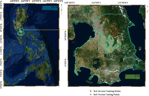
The study area is located between 13°30′00″ N to 15°00′00″ N and 120°00′00″ E to 122°00′00″ E known as Southern Luzon in the Philippines (Figure 1) covering 10,997 km². In selecting the study area, attempts were made to select an area that has varieties of each soil erosion conditioning factor. In the east, the rainfall is more or less evenly distributed throughout the year. The average annual rainfall ranges between 2000 mm in the west to 4000 mm in the east (http://www1.pagasa.dost.gov.ph/index.php/climate/climatological-normals). The high rainfall associated with the passage of tropical cyclones, averaging 19.4 per year (Cinco et al. 2016), is partly responsible for the active erosion observed in the area (Adornado et al. 2009, Atienza and Hipolito 2010). The area of interest is part of a tectonically and volcanically active zone, comprising of several calderas and stratovolcanoes, and hundreds of monogenetic volcanic edifices such as maars and scoria cones (Nelson et al. 2000). Faults and fractures transect the area. The geologic setting of the area explains in part the high erosion in the area.

Figure 1. Study area location (source: ESRI Basemap).

The area of interest includes a major river basin (i.e. the Pasig-Laguna de Bay river basin) and several critical watersheds. The Laguna de Bay and adjacent regions are a principal rice bowl of the Philippines. The area includes the two most populous regions: National Capital region (including Metro Manila) and Calabarzon (consisting of the provinces of Cavite, Laguna, Batangas, Rizal and Quezon) with a total population of 27.3 million (https://www.psa.gov.ph/content/highlights-philippine-population-2015-census-population). These areas have experienced rapid industrial growth. Selected areas in the Calabarzon have been and are being developed to support the accelerating needs for space and economic, social and environmental resources for the National Capital region. The two regions account for nearly 54% of Philippine domestic production for the period 2010–2015 National Economic and Development Authority (2017). Deforestation due to logging, fires, expanding agriculture or conversion to built-up areas is considered a major cause of erosion (Maohong 2012). The selected study area has an altitude from 1 m to 2100 m a.s.l; for lithology, the study area had 21 different geological units, and for LULC, our selected study area had 17 different types of LULC.

3.2. Spatial data-sets

3.2.1. Inventory factors

In this study, 70% of the soil erosion layer, as an inventory factor obtained from the Bureau of Soil and Water Management (BSWM), was used for model training while the remainder (30%) was reserved for validation purposes (Figure 1).

3.2.2. Conditioning factors

One of the challenging tasks in natural hazard simulation and modelling is to select the most relevant contributing factors. There is no specific framework that defines the sufficient numbers and types of the parameters. These factors are usually selected by the user based on the relevance and influences of those factors on soil erosion occurrence. Moreover, there are several topographical, hydrological and geological factors that are cited and frequently used by other researchers (Conoscenti et al. 2008; Krishna Bahadur 2009; Conforti et al. 2011; Feizizadeh and Blaschke 2013; Altaf et al. 2014). In the current research ten factors were chosen to be used in the analysis, which have considerable impact on generating soil erosion. Their influences could directly or indirectly cause erosion in the terrain. Ten conditioning factors belonging to the current time: (1) altitude, (2) slope, (3) aspect, (4) curvature, (5) lithology, (6) distance from river, (7) distance from road, (8) soil type, (9) LULC and (10) rainfall, for the two time periods, current time and 2100 based on the A2 scenario and CSIRO global climate model (available at http://www.worldclim.org/), with a grid cell size 30 × 30 m were used to run the FR and EBF models.

3.2.2.1. Altitude, slope, aspect and curvature

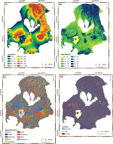
Altitude is one of the most important factors in soil erosion studies as it affects the erosive power of the surface runoff (Conoscenti et al. 2008). Slope, aspect and curvature are the physical characteristics of the terrain. The impact of slope (Ziadat and Taimeh 2013), aspect (Gabarrón-Galeote et al. 2013; Raouf et al. 2017) and curvature (Perreault et al. 2016) on soil erosion has been studied by many researchers. Steep lands increase the velocity of the runoff and reduce the absorption time. On the other hand, aspect direction of the land impacts on the amount of the sunshine and precipitation that the terrain receives (Mansor et al. 2004; Nadal-Romero et al. 2014; Rodrigo Comino et al. 2017). Altitude, slope, aspect and curvature layers were generated from DEM as shown in Figures 2(a), (b), (c) and (d), respectively. In the current research, altitude and slope maps ranged from 0 to 2100 m above sea level and 0 to 71 degrees, respectively. As can be seen in Figures 2(a) and (b), the high elevated and steep regions are located in the north and northeast of the catchment. Moreover, the aspect map represents nine slope directions and curvature thematic map contains three classes of convex, flat and concave, illustrating the shape or curvature of the slope.

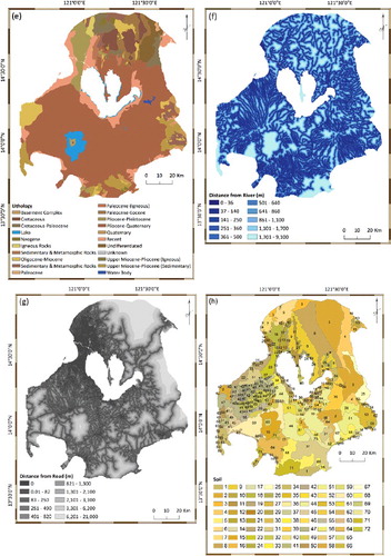
Figure 2. Soil erosion conditioning factors: (a) altitude, (b) slope, (c) aspect, (d) curvature, (e) geology, (f) distance from river, (g) distance from road, (h) soil type (refer to Table S1), (i) LULC and (j) rainfall for current time.

3.2.2.2. Lithology

Lithology is one of the major factors in soil erosion studies due to its impact on the presence of soil erosion. Research undertaken by Conforti et al. (2011) showed that this factor plays a critical role in impacting soil erosion. Water permeability, strength etc. are the characteristics that vary from one lithology type to another (Cerda 1999, Martínez-Hernández et al.). Therefore, this factor was used as one of the most influential factors in this study. The lithology layer, obtained from Mines and Geoscience Bureau, contained different types of lithology as shown in Figure 2(e).

3.2.2.3. Distance from river and road

Distance from river is also a major conditioning factor due to the impact of water on soil erosion (Panagos et al. 2012). Road construction requires cutting the terrain which causes instability in the land (Swanson and Dyrness 1975). These impervious materials will speed up the water flow and cause soil erosion in the regions around. Distance from river and road layers were generated by Euclidean distance tool and divided into ten classes using quantile method as shown in Figures 2(f) and (g), respectively.

3.2.2.4. Soil type

Different soil types have different characteristics, such as absorption capacity, empty spaces among the particles etc. which considerably influence the soil erosion potential of the region (Heshmati et al. 2013). The soil layer, obtained from BSWM, contained 72 different soil types as shown in Figure 2(h). By looking at both Figures 1 and 2(h) it is evident that most of the soil erosion locations mainly fall in three classes of soil, including Novaliches clay loam, Antipolo clay and Antipolo soils (undifferentiated).

3.2.2.5. Land use/cover (LULC)

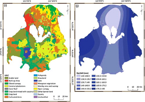
Zhou et al. (2008) assessed the effect of vegetation on soil erosion and concluded that dense vegetation cover can considerably reduce the surface runoff speed and consequently prevent soil erosion occurrence in the region. Moreover, the roots of the trees strengthen the soil structure. On the other hand, deforestation and existence of the impervious surfaces promote the water flow and create soil loss in the area (Ochoa-Cueva et al. 2015). The LULC layer, obtained from BSWM, contained 17 different types of LULC as shown in Figure 2(i). Cultivated Area mixed with brushland/grassland area has experienced the highest extent of soil erosion as can be seen in Figures 1 and 2(i).

3.2.2.6. Rainfall (current time and 2100)

The impact of rainfall on soil erosion occurrence has been studied by a variety of researchers (Martínez Casasnovas et al. 2002). Nearing et al. (2005) studied different soil erosion scenarios due to the changes in precipitation and LULC. Their results indicated that the sensitivity values for runoff and erosion were generally greater for rainfall changes as opposed to LULC changes. The current rainfall data was obtained from the Philippine Atmospheric Geophysical and Astronomical Service Administration (PAGASA) while the projected rainfall data for 2100 was obtained from CLIMOND database (Kriticos et al. 2012). Figure 2(j) represents rainfall for the current time.

As a requirement of both FR and EBF method, each factor needs to be categorized prior to the analysis (Yilmaz 2009b; Althuwaynee et al. 2012b; Jebur et al. 2014b). The reason for this is that the BSA method evaluates the impact of every class of each conditioning factor on the soil erosion occurrence. Regarding the used classification scheme, there are four classification techniques of quantile, natural breaks, equal intervals and standard deviations available that can be used to categorize the scaled data (Ayalew and Yamagishi 2005) and has been frequently used by researchers in the field of natural hazard (Ayalew et al. 2004; Ayalew and Yamagishi 2005; Papadopoulou-Vrynioti et al. 2013; Mojaddadi et al. 2017). Selection of each method depends on the nature of the data used and the application of the project. One of the disadvantages of equal interval method is that it places widely different values into the same class. On the other hand, some classes might only carry a few pixels (Chung and Fabbri 2003). Other classification methods, such as standard deviation or natural break, follow specific framework and manipulate the classes into non-user defined categories. However, in this research, in order to have a reliable judgment regarding the impact of every class of each factor on soil erosion occurrence we attempted to reduce the influence of classification algorithm on the conditioning factors classes as much as possible. In some population analysis projects where the goal is to find a big jump in the data, natural break technique is highly recommended (Xiao et al. 2006), while in this research, this method would not be efficient. Hence, quantile-based classification technique was found to be more appropriate to classify the factors in this study. This method groups equal number of pixels (area) into each group without any interference in the separation of the pixels.

3.3. Models

3.3.1. Frequency ratio (FR) model

The FR model is based on the ratio of the probability occurrence to non-occurrence for a specific event (Lee and Pradhan 2006b; Mojaddadi et al. 2017). Alternatively, it may be described as the spatial correlation between specific incidents and the conditioning factors related to its occurrence (Alon and Spencer 2004). These correlations were derived by application of the FR model (Demir et al. 2013). FR is a BSA model that can assist in modelling the research area both logically and physically. In terms of analysis of soil erosion, if A represents the event incidents and B the related spatial factor, the FR for B establishes the ratio of conditional probability. In terms of the theory of probability, conditional probability describes the likelihood of occurrence of an incident, when another incident will occur or has already occurred (Lee and Pradhan 2006b). When the ratio exceeds 1, the related conditioning factor shows a greater correlation with the occurrence of soil erosion, while a ratio less than 1 indicates less correlation with an occurrence. FR was calculated using Excel and ArcGIS software.

For calculating a hazard index for soil erosion, individual conditioning factors were reclassified in terms of acquired weights and the factors were summed.

3.3.2. Evidential belief function (EBF) known as Dempster–Shafer theory (DST)

The Dempster–Shafer theory (DST) of evidence, developed by Dempster (Dempster 1967), is a generalization of the Bayesian theory of subjective probability (Feizizadeh and Blaschke 2013). Its major advantages are its relative flexibility in accepting uncertainty and the capacity to combine beliefs from multiple sources of evidence (Thiam 2005; Feizizadeh and Blaschke 2014). DST estimates the closeness with which the evidence proves the hypothesis valid (Feizizadeh et al. 2014b), as opposed to estimating the probability that it is valid (Pearl 1990), and has been successfully applied in many fields using a GIS (Malpica et al. 2007).

Suppose that there is a set of soil erosion conditioning factors C = (C_i, i = 1, 2, 3, …, n), comprising mutually exclusive and exhaustive factors C_i. C is known as the frame of discernment. A basic probability assignment is a function m: P(C)→[0, 1].

P(C) is the set of all subsets of C, including the empty set and C itself. This function is also called a mass function and satisfies m(Ф) = 0 and $\sum _{AC}m \left(A\right)= 1$, where Ф is an empty set and A is any subset of C. The m(A) measures the degree to which the evidence supports A and it is denoted by Bel (A), a belief function.

There are four basic EBF functions used: (1) Bel (degree of belief), (2) Dis (degree of disbelief), (3) Unc (degree of uncertainty) and (4) Pls (degree of plausibility) (Feizizadeh et al. 2014a). Bel and Pls present the lower and upper bounds of the probability for the proposition (Awasthi and Chauhan 2011; Althuwaynee et al. 2012a); Unc is the difference between the belief and the plausibility, while Unc presents the ignorance. Dis is the belief of the proposition being false on given evidence.

Dis = 1 − Pls or 1 − Unc − Bel, and we always get Bel + Unc + Dis = 1. For a case of C_ij with no soil erosion occurrence indicating that Bel = 0, Dis is reset to zero, even if Dis is not (Carranza et al. 2008). The estimation of EBF can be based on subjective judgment or it can be data-driven (Srivastava et al. 2011). By overlaying the soil erosion inventory map (L) on each of the ten maps of soil erosion conditioning factors, we determined the number of pixels with, and without, soil erosion for each factor class. Assuming that N(L) is the total number of soil erosion pixels and N(C) is the total number of pixels in the study area, Cij is the j-th class attribute of the soil erosion conditioning factors C_i (i = 1, 2, …, n), N(C_ij) is the total number of pixels in the class C_ij and N(L∩C_ij) is the number of soil erosion pixels in C_ij. According to (Carranza and Hale 2003), data-driven estimation of EBFs may be undertaken by:(1) $Bel \left(C_{ij}\right)= \frac{W_{C_{ij} \left(\mathrm{soil erosion}\right)}}{{\sum }_{j = 1}^n W_{C_{ij} \left(\mathrm{soil erosion}\right)}}$(1) (2) $W_{C_{ij} \left(\mathrm{soil erosion}\right)}= \frac{\raisebox{1ex}{$N(L\bigcap C_{ij})$}\!\left/ \!\raisebox{-1ex}{$N\left(L\right)$}\right.}{\raisebox{1ex}{${\left[N \right(C}_{{ }_{ij}})-N (L\bigcap C_{ij}\left)\right]$}\!\left/ \!\raisebox{-1ex}{$\left[N \right(C)-N (L\left)\right]$}\right.}$(2) (3) $Dis \left(C_{ij}\right)= \frac{W_{C_{ij} \left(\mathrm{without soil erosion}\right)}}{{\sum }_{j = 1}^n W_{C_{ij} (\mathrm{non}-\mathrm{ soil erosion})}}$(3) where(4) $W_{C_{ij} \left(\mathrm{without soil erosion}\right)}= \frac{\raisebox{1ex}{$[N \left(C_{ij}\right)-N (L\bigcap C_{ij}\left)\right]$}\!\left/ \!\raisebox{-1ex}{$N \left(L\right)$}\right.}{\raisebox{1ex}{${\left[N \right(C}_{ })-N \left(L\right)-N \left(C_{ij}\right)+N (L\bigcap C_{ij}\left)\right]$}\!\left/ \!\raisebox{-1ex}{$\left[N \right(C)-N (L\left)\right]$}\right.}$(4)

The numerator in equation (2)(2) $W_{C_{ij} \left(\mathrm{soil erosion}\right)}= \frac{\raisebox{1ex}{$N(L\bigcap C_{ij})$}\!\left/ \!\raisebox{-1ex}{$N\left(L\right)$}\right.}{\raisebox{1ex}{${\left[N \right(C}_{{ }_{ij}})-N (L\bigcap C_{ij}\left)\right]$}\!\left/ \!\raisebox{-1ex}{$\left[N \right(C)-N (L\left)\right]$}\right.}$(2) is the proportion of soil erosion pixels in factor class C_ij; the numerator in equation (4)(4) $W_{C_{ij} \left(\mathrm{without soil erosion}\right)}= \frac{\raisebox{1ex}{$[N \left(C_{ij}\right)-N (L\bigcap C_{ij}\left)\right]$}\!\left/ \!\raisebox{-1ex}{$N \left(L\right)$}\right.}{\raisebox{1ex}{${\left[N \right(C}_{ })-N \left(L\right)-N \left(C_{ij}\right)+N (L\bigcap C_{ij}\left)\right]$}\!\left/ \!\raisebox{-1ex}{$\left[N \right(C)-N (L\left)\right]$}\right.}$(4) is the proportion of soil erosion pixels that do not occur in factor class C_ij; the denominator in equation (2)(2) $W_{C_{ij} \left(\mathrm{soil erosion}\right)}= \frac{\raisebox{1ex}{$N(L\bigcap C_{ij})$}\!\left/ \!\raisebox{-1ex}{$N\left(L\right)$}\right.}{\raisebox{1ex}{${\left[N \right(C}_{{ }_{ij}})-N (L\bigcap C_{ij}\left)\right]$}\!\left/ \!\raisebox{-1ex}{$\left[N \right(C)-N (L\left)\right]$}\right.}$(2) is the proportion of non-soil erosion pixels in factor class C_ij; and the denominator in equation (4)(4) $W_{C_{ij} \left(\mathrm{without soil erosion}\right)}= \frac{\raisebox{1ex}{$[N \left(C_{ij}\right)-N (L\bigcap C_{ij}\left)\right]$}\!\left/ \!\raisebox{-1ex}{$N \left(L\right)$}\right.}{\raisebox{1ex}{${\left[N \right(C}_{ })-N \left(L\right)-N \left(C_{ij}\right)+N (L\bigcap C_{ij}\left)\right]$}\!\left/ \!\raisebox{-1ex}{$\left[N \right(C)-N (L\left)\right]$}\right.}$(4) is the proportion of non-soil erosion pixels in other attributes outside factor class of C_ij. Parameter W_Cij (soil erosion) is the weight of C_ij that supports the belief that soil erosion is more present than absent. Parameter W_Cij (without soil erosion) is the weight of C_ij that supports the belief that soil erosion is more absent than present.

EBF functions were measured using Excel and ArcGIS software. Once the EBF function had been calculated for all the soil erosion conditioning factors, the Dempster's rule of combination was used and applied using raster calculator in ArcGIS to obtain the four integrated EBFs. The formulae for combining of two soil erosion conditioning factors C₁ and C₂ are as follows (Carranza et al. 2005):(5) ${Bel}_{C_1{C}_2}=\frac{{Bel}_{C_1}{Bel}_{C_2}+{Bel}_{C_1}{Unc}_{C_2}+{Bel}_{C_2}{Unc}_{C_1}}{1-{Bel}_{C_1}{Dis}_{C_2}-{Dis}_{C_1}{Bel}_{C_2}}$(5) (6) ${Dis}_{C_1{C}_2}=\frac{{Dis}_{C_1}{Dis}_{C_2}+{Dis}_{C_1}{Unc}_{C_2}+{Dis}_{C_2}{Unc}_{C_1}}{1-{Bel}_{C_1}{Dis}_{C_2}-{Dis}_{C_1}{Bel}_{C_2}}$(6) (7) ${Dis}_{C_1{C}_2}=\frac{{Dis}_{C_1}{Dis}_{C_2}+{Dis}_{C_1}{Unc}_{C_2}+{Dis}_{C_2}{Unc}_{C_1}}{1-{Bel}_{C_1}{Dis}_{C_2}-{Dis}_{C_1}{Bel}_{C_2}}$(7)

Integrated EBF of the soil erosion conditioning factors are implemented sequentially using equations 5(5) ${Bel}_{C_1{C}_2}=\frac{{Bel}_{C_1}{Bel}_{C_2}+{Bel}_{C_1}{Unc}_{C_2}+{Bel}_{C_2}{Unc}_{C_1}}{1-{Bel}_{C_1}{Dis}_{C_2}-{Dis}_{C_1}{Bel}_{C_2}}$(5) , 6(6) ${Dis}_{C_1{C}_2}=\frac{{Dis}_{C_1}{Dis}_{C_2}+{Dis}_{C_1}{Unc}_{C_2}+{Dis}_{C_2}{Unc}_{C_1}}{1-{Bel}_{C_1}{Dis}_{C_2}-{Dis}_{C_1}{Bel}_{C_2}}$(6) and 7(7) ${Dis}_{C_1{C}_2}=\frac{{Dis}_{C_1}{Dis}_{C_2}+{Dis}_{C_1}{Unc}_{C_2}+{Dis}_{C_2}{Unc}_{C_1}}{1-{Bel}_{C_1}{Dis}_{C_2}-{Dis}_{C_1}{Bel}_{C_2}}$(7) . Table S1 shows the estimated EBFs for the ten soil erosion conditioning factors.

4. Results

We examined ten conditioning factors together with the soil erosion inventory map. As mentioned earlier, each factor was assessed individually in both FR and EBF. Table S1 shows the estimated EBF and FR for the ten soil erosion conditioning factors, individually. It should be noted that the derived weights for each factor is only specific to this study area. Applying EBF and FR for other case studies may lead to similar or different outcomes. The reason for this is that each catchment has different topographical, hydrological and geological conditions that might affect soil erosion through different interactions of factors.

4.1. Conditioning factors

4.1.1. Altitude

The EBF outputs on this conditioning factor indicated that the range of altitude between 230 and 2100 m received high weights. The belief (Bel) value achieved by EBF method had the highest value (61) at altitudes from 221–290 m while it was 16 and 13 at altitudes from 300 to 380 and 511 to 2100 m, respectively. The FR output also agreed that the highest FR weights were measured for the range of altitude from 221 to 290 m, while altitudes from 300 to 380 and 511 to 2100 m had a moderate FR weights (Table S1).

4.1.2. Slope, aspect and curvature

The outputs on slope using FR indicated that classes of 14°–18°, 19°–25° and 26°–71° acquired weights of 2, 4 and 2, respectively. Furthermore, they produced EBF results of 19, 39 and 26 for Bel value, respectively.

The three highest FR values of 3, 1 and 1 were related to the classes of south-east, south and north-west of aspect layer, respectively. The same classes acquired the highest Bel values through EBF method. Curvature-wise, there was agreement and disagreement between FR and EBF outputs. For example, both methods agreed that concave curvature had the highest value while only EBF projected that convex curvature had the second highest Bel value (Table S1).

4.1.3. Lithology

The class of ‘Cretaceous-Paleocene and Igneous Rocks’ acquired the FR weights of 11 and 13 and Bel weights of 28 and 31 through EBF method, respectively, indicating the higher correlation among these classes and soil erosion. For this conditioning factor, the extent of agreement between FR and EBF outputs exceeded the extent of disagreement (Table S1).

4.1.4. Distance from river and road

For this factor, the highest FR weights of 3, 1 and 1 represented the classes of 501–640 , 641–860 and 1101–1700 m, respectively. Furthermore, the Bel weights of 38, 18, and 11, respectively, verified the results of FR. On river and road conditioning factors, the extent of disagreement between FR and EBF outputs exceeded agreement; for example, on river factor EBF estimated a high correlation among all ten classes of distance from the river and soil erosion, while FR estimated only three classes (Table S1).

4.1.5. Soil type

Our results showed that for soil type, the highest FR weights of 9 and 5 belonged to the class of Antipolo soils and Antipolo clay, which also produced the highest Bel weights of 46 and 23. Our results indicate that these two soil types have strong correlation with soil erosion occurrence, while the remainder of soil types within the study area does not exhibit a strong relationship.

4.1.6. Land use/cover (LULC)

Our result on this conditioning factor shows the highest FR weight of 67 for the class of grassland, which is verified by the EBF Bel weight of 97. Comparing the FR and EBF outputs on the remaining classes, our result indicates significant consistency and agreement between these model outputs.

4.1.7. Rainfall for current time

Our finding on this conditioning factor revealed that the highest FR weights of 4 and 1 represent the classes of 120–138.9 and 138.9–139.7 mm/day, which are verified by EBF Bel weight of 66 and 25 for the same classes of rainfall. Comparing the FR and EBF outputs for the remainder of classes, some inconsistency and disagreement was found for the classes of 159.2–159.8 and 169.1–169.9.

4.2. Probability index maps and susceptibility maps

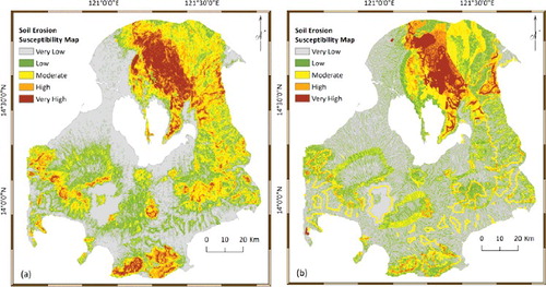
The soil erosion probability index maps produced by EBF and FR methods are shown in Figures 3(a) and (b), respectively. The soil erosion probability ranges from 0 to 1, with 0 representing no probability and 1 representing 100% probability. For producing susceptibility maps, as well as improving the visual interpretation of area susceptibility, probability maps need to be categorized into specific classes (Umar et al. 2014). A variety of classification techniques, such as equal interval, standard deviation, natural break and quantile, is available; the selection of which needs to be based on the data characteristics and research objectives. For data with normal distribution, equal interval is suitable, whereas standard deviation classifies data according to a fixed number of classes. With a data-set exhibiting a sudden or big jump, natural break is suitable. Having researched the literature, quantile is the most popular choice of classification method for susceptibility mapping (Umar et al. 2014). We used the quantile method to produce the susceptibility classes and classified our probability indices into five zones of susceptibility: very low, low, moderate, high and very high for both EBF and FR outputs (Figures 4(a) and (b)).

Figure 3. Soil erosion probability index maps achieved by (a) EBF and (b) FR methods.

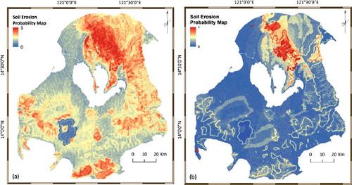
Figure 4. Soil erosion susceptibility maps achieved by (a) EBF and (b) FR methods.

5. Model validation and comparison of EBF and RF models

The soil erosion hazard analysis was executed and validated using known soil erosion locations (Figure 1). Natural hazards modelling (i.e. soil erosion) is an appropriate technique to identify the extent and the location of natural threats in advance; however, identifying the accuracy and extent of the predictive ability is vital once model training is completed (Nefeslioglu et al. 2013). For this the area under curve (AUC) is generally used to determine the quality of the probabilistic model by describing its ability to reliably predict the occurrence or non-occurrence of hazards (i.e. soil erosion) event (Feizizadeh et al. 2014c). Thus the AUC method was used for validation, based on the training and testing soil erosion locations (Pradhan et al. 2010). While training soil erosion locations were used to generate the hazard model, the results of validation using this data does not represent the real efficiency of the developed model. The prediction rate was measured to establish how efficiently the two models and selected conditioning factors predicted soil erosion (Feizizadeh et al. 2014c). AUC can assess prediction accuracy qualitatively by sorting the calculated values of all cells in the study area into a descending order, thus ranking each prediction hierarchically. Thereafter, the values of cells were divided into 100 classes with 1% accumulation intervals. The verification results for both methods (FR and EBF) are shown in Figure 4. The AUC results showed 72.8% and 85.7% success rates for FR and EBF, respectively, while a 70.6% and 83.1% prediction rate was achieved, respectively (Figures 5(a) and (b)). The efficiency of both methods was compared quantitatively and the results revealed that EBF has greater prediction capability than FR. Thus, we chose the EBF method to predict future soil erosion probability to produce the susceptibility map for 2100, as shown in Figure 6.

Figure 5. AUC success rate and prediction rate of (a) EBF and (b) FR methods.

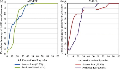
Figure 6. Projected soil erosion probability index map (left-hand side map) and susceptibility map (right-hand side map) by 2100 through EBF method.

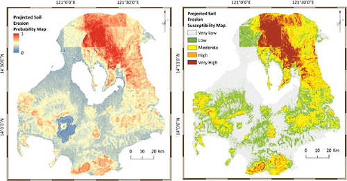
Comparing the very high susceptibility class for current time (Figure 4(a)) and 2100 (Figure 6, right-hand side map), our EBF results indicated an increase in soil erosion in the northern part of the study area, no changes in the eastern regions and a decrease in the western and southern regions. A similar time frame comparison for the low susceptibility class showed an increase between current time and 2100, particularly in the regions between 121°0′00″ E and 121° 10′00″ E, and 14°45′00″ N and 14°55′00″ N. An increase in the moderate susceptibility class in all four corners of the study area was found between current time and 2100 (Figure 4(a) and Figure 6, right-hand side map). Moreover, comparing the susceptibility maps of current (FR-derived) and future (EBF-derived) almost similar changes of increase of soil erosion incidences in the north and decrease in the south part of the study area can be seen.

6. Discussion

Although a variety of statistical methods have been proposed and tested in the field of natural hazards, the application and proficiency of EBF in soil erosion susceptibility mapping has not been examined sufficiently. This study undertook a comparative assessment of the proficiency of the EBF and FR statistical methods in mapping the soil erosion probability and susceptibility for the current time. Thereafter, based on AUC validation, establishing that EBF had a better prediction rate, this model was chosen to generate soil erosion probability and susceptibility for 2100. The maps produced can assist the national departments and agricultural organizations establish regions that are highly or moderately susceptible to soil erosion in order to plan and implement prevention or reduction measures, as well as prepare for consequential occurrences such as floods and landslides. Susceptibility maps provide the foundation for further analytical tools, such as hazard and risk mapping. However, it should be noted that the projected extent of soil erosion is based on the LULC, road and river layers for the current time and these layers may change in the future, however this point was not examined in this study as it is impossible to have a high degree of predictability of such layers in the future.

The EBF outputs on altitude conditioning factor indicated that altitudes from 221 to 2100 m had a strong correlation with soil erosion occurrence, which can be due to the greater instability of ground at higher elevations. Slope, aspect, curvature and soil types describe the physical characteristics of the terrain. Our results showed that these factors have specific influence on the initiation of soil erosion. For example, moisture preservation and distribution of vegetation amount are related to the slope aspect, which has a direct impact on soil strength and susceptibility to soil erosion. This finding is supported by a variety of researches. The condition and characteristic of soil and vegetation are highly related to the slope aspect factor which subsequently influences the soil erosion susceptibility of the terrain (Perreault et al. 2016). Yetemen et al. (2015) described the correlation between aspect and vegetation for the Northern Hemisphere. They found that the south-facing slopes were usually warmer and drier, have a thinner soil layer and are less densely vegetated than north-facing slopes. The correlation between the slope aspect directions and vegetation coverage has been studied in detail by Nadal-Romero et al. (2014), Rodrigo Comino et al. (2017) and Gabarrón-Galeote et al. (2013). Gabarrón-Galeote et al. (2013) stated that the species diversity and plant abundance are highly affected by the slope aspect condition of the study area. Different patterns of soil movement have been observed in a study by Rodrigo Comino et al. (2017), as the west side of their studied hillslope had higher soil movement than the east region. The lowest soil erosion potential was observed on the eastern aspect.

The projected susceptibility map was compared with the 2 current susceptibility maps derived from EBF and FR methods. Compared to both current susceptibility maps, the future map showed an increase in soil erosion susceptibility in the north and decrease in the south parts of the study area. The increase in class of very high and moderate soil erosion susceptibility for 2100 can be explained by potential changes in the rainfall layer as a consequence of climate change. However, it should be mentioned that as rainfall changes, LULC and the locations of rivers and roads could change and, consequently, the level of soil erosion susceptibility. Thus, the result of an increase in the very high and moderate classes of soil erosion susceptibility in the study area is based on available data for the rainfall layer for current time and, as obtained from CLIMOND database, by 2100.

Our results show the efficiency of EBF in soil erosion studies and, to the best of our knowledge, this technique has not been previously utilized for the generation of soil erosion susceptibility mapping. However, as mentioned earlier, both BSA and MSA have inherent weaknesses and further research is needed to find appropriate solutions for these techniques in order to increase the reliability and speed of hazard analysis of these models. Ensemble modelling could be one of the applicable solutions for this matter which is a technique of combining two or more algorithms and enhancing their performance through this integration (Althuwaynee et al. 2014; Tehrany et al. 2015). Often, the process starts by performing one method and utilizes the outcome and enters them as input in the second model (Youssef et al. 2015). Using this approach ,disadvantages of individual methods can be reasonably reduced. A future study would be focusing on improving and proposing novel ensemble techniques in soil erosion susceptibility mapping.

It is important to note that the accuracy of estimations of soil loss is dependent on the accuracy with which conditioning factor values are calculated (Dou et al. 2015). Beyond the establishment of the class, it is essential to understand conditioning factors that impact most on soil erosion. Once the conditioning factors and associated severity of impact is established, the information is invaluable in terms of the formulation of conservation planning to protect areas at risk. Planning must extend beyond the direct onsite impact of soil erosion to curtail the consequential downstream impact of transported sediments. These results contribute to the promulgation of public awareness of such geo-hazards in order to reduce life and economic losses.

As it has been mentioned earlier, the projected extent of soil erosion in this study is based on the LULC, road and river layers for the current time and these layers may change in the future. This can be an interesting future research topic to include the expected changes in LULC through considering the governmental city expansion plans. It is also recommended to examine and compare the performance of an ensemble or integrated EBF technique with other statistical methods in the field of soil erosion mapping.

7. Conclusion

This research aimed to use two of the most popular statistical techniques of FR and EBF to map the current soil erosion susceptible areas in a hazardous catchment in Philippines, and subsequently utilize the most accurate approach to project the future susceptible locations in the study area by including an additional conditioning factor of rainfall belonging to the year 2100.

(1)	Conditioning factors were selected in terms of their relevance and used in the construction of spatial layers, including: altitude, slope, aspect, curvature, lithology, distance from river, distance from road, soil type, LULC and rainfall for current time and 2100 formed the data-set.
(2)	The inventory map was divided into training and testing data-sets.
(3)	EBF and FR were applied using the training locations and correlations of classes and conditioning factors were evaluated.
(4)	Validation was performed using AUC method which showed success rates of 72.8% and 85.7% for FR and EBF, respectively. In addition, the results showed that the FR model (70.6%) has less accuracy of prediction than the EBF model (83.1%). This shows the superior capabilities of MSA over the BSA, with the results of EBF model having higher prediction accuracies than the probabilistic FR model in the process of soil erosion hazard mapping.

Statistical modelling is advantageous for its simplicity and user-friendly qualities. It is also capable of processing large quantities of data in a GIS environment relatively quickly. Sustainable urban development is dependent on knowledge of the potential impacts of soil erosion hazards and the control thereof. Thus, research into the susceptibility and hazard mapping of regions supports sustainability and is valued by engineers, planners and developers in terms of LULC planning and slope management. This research shows that the techniques developed here can be used for erosion modelling; however, it must be emphasized that the impact of each of the factors may be different for different case study sites due to the different interactions between factors.

Acknowledgements

Thanks to two anonymous reviewers for their valuable and critical comments which helped us to improve the quality of earlier version of the manuscript.

Disclosure statement

No potential conflict of interest was reported by the authors.

References

- Adornado HA, Yoshida M, Apolinares HA. 2009. Erosion vulnerability assessment in REINA, Quezon Province, Philippines with raster-based tool built within GIS environment. Agr Inf Res. 18:24–31.
- Alam M, Hussain RR, Islam AS. 2016. Impact assessment of rainfall-vegetation on sedimentation and predicting erosion-prone region by GIS and RS. Geomat Nat Haz Risk. 7:667–679.
- Alon N, Spencer JH. 2004. The probabilistic method. New York: Wiley.
- Altaf S, Meraj G, Romshoo SA. 2014. Morphometry and land cover based multi-criteria analysis for assessing the soil erosion susceptibility of the western Himalayan watershed. Environ Monit Assess. 186:8391–8412.
- Althuwaynee O, Pradhan B, Lee S. 2012a. Application of an evidential belief function model in landslide susceptibility mapping. Comput Geosci. 44:120–135.
- Althuwaynee OF, Pradhan B, Lee S. 2012b. Application of an evidential belief function model in landslide susceptibility mapping. Comput Geosci. 44:120–135.
- Althuwaynee OF, Pradhan B, Park HJ, Lee JH. 2014. A novel ensemble decision tree-based CHi-squared automatic interaction detection (CHAID) and multivariate logistic regression models in landslide susceptibility mapping. Landslides. 11:1063–1078.
- Asio VB, Jahn R, Perez FO, Navarrete IA, Abit SM Jr. 2009. A review of soil degradation in the Philippines. Ann Trop Res. 31:69–94.
- Atienza EF, Hipolito DM. 2010. Challenges on risk management of sediment-related disasters in the Philippines. Int J Eros Control Eng. 3:85–91.
- Aurit MD, Peterson RO, Blanford JI. 2013. A GIS analysis of the relationship between sinkholes, dry-well complaints and groundwater pumping for frost-freeze protection of winter strawberry production in Florida. Plos One. 8:e53832.
- Awasthi A, Chauhan S. 2011. Using AHP and Dempster–Shafer theory for evaluating sustainable transport solutions. Environ Model Softw. 26:787–796.
- Ayalew L, Yamagishi H. 2005. The application of GIS-based logistic regression for landslide susceptibility mapping in the Kakuda-Yahiko Mountains, Central Japan. Geomorphology. 65:15–31.
- Ayalew L, Yamagishi H, Ugawa N. 2004. Landslide susceptibility mapping using GIS-based weighted linear combination, the case in Tsugawa area of Agano River, Niigata Prefecture, Japan. Landslides. 1:73–81.
- Calderhead A, Therrien R, Rivera A, Martel R, Garfias J. 2011. Simulating pumping-induced regional land subsidence with the use of InSAR and field data in the Toluca Valley, Mexico. Adv Water Resour. 34:83–97.
- Carranza E, Hale M. 2003. Evidential belief functions for data-driven geologically constrained mapping of gold potential, Baguio district, Philippines. Ore Geology Reviews. 22:117–132.
- Carranza E, Hale M, Faassen C. 2008. Selection of coherent deposit-type locations and their application in data-driven mineral prospectivity mapping. Ore geology reviews. 33:536–558.
- Carranza E, Woldai T, Chikambwe E. 2005. Application of data-driven evidential belief functions to prospectivity mapping for aquamarine-bearing pegmatites, Lundazi district, Zambia. Nat Resour Res. 14:47–63.
- Cerda A. 1999. Parent material and vegetation affect soil erosion in eastern Spain. Soil Sci Soc Am J. 63:362–368.
- Chang Z, Zhang J, Guo Q, Gong L. 2004. Study on land subsidence evolvement tendency by means of “integrated DInSAR”. Proceedings of the IEEE International Geoscience and Remote Sensing Symposium (IGARSS'04); Anchorage (AK): IEEE. doi:10.1109/IGARSS.2004.1368944.
- Chaussard E, Wdowinski S, Cabral Cano E, Amelung F. 2014. Land subsidence in central Mexico detected by ALOS InSAR time-series. Remote Sens Environ. 140:94–106.
- Choi JK, Kim KD, Lee S, Won JS. 2010. Application of a fuzzy operator to susceptibility estimations of coal mine subsidence in Taebaek City, Korea. Environ Earth Sci. 59:1009–1022.
- Chung CJF, Fabbri AG. 2003. Validation of spatial prediction models for landslide hazard mapping. Nat Hazards. 30:451–472.
- Cinco TA, Guzman RG, Ortiz AMD, Delfino RJP, Lasco RD, Hilario FD, Juanillo EL, Barba R, Ares ED. 2016. Observed trends and impacts of tropical cyclones in the Philippines. Int J Climatol. 36:4638–4650.
- Clerici A, Perego S, Tellini C, Vescovi P. 2002. A procedure for landslide susceptibility zonation by the conditional analysis method. Geomorphology. 48:349–364.
- Conforti M, Aucelli PP, Robustelli G, Scarciglia F. 2011. Geomorphology and GIS analysis for mapping gully erosion susceptibility in the Turbolo stream catchment (Northern Calabria, Italy). Nat hazards. 56:881–898.
- Conoscenti C, Di Maggio C, Rotigliano E. 2008. Soil erosion susceptibility assessment and validation using a geostatistical multivariate approach: a test in Southern Sicily. Nat Hazards. 46:287–305.
- Demir G, Aytekin M, Akgün A, İkizler SB, Tatar O. 2013. A comparison of landslide susceptibility mapping of the eastern part of the North Anatolian Fault Zone (Turkey) by likelihood-frequency ratio and analytic hierarchy process methods. Nat Hazards. 65:1481–1506.
- Dempster A. 1967. Upper and lower probabilities induced by a multivalued mapping. Ann Math Stat. 38:325–339.
- Ding X, Liu G, Li Z, Li Z, Chen Y. 2004. Ground subsidence monitoring in Hong Kong with satellite SAR interferometry. Photogramm Eng Remote S. 70:1151–1156.
- Dou J, Bui DT, Yunus AP, Jia K, Song X, Revhaug I, Xia H, Zhu Z. 2015. Optimization of causative factors for landslide susceptibility evaluation using remote sensing and GIS data in parts of Niigata, Japan. PloS One. 10:e0133262.
- Feizizadeh B, Blaschke T. 2013. GIS-multicriteria decision analysis for landslide susceptibility mapping: comparing three methods for the Urmia lake basin, Iran. Nat hazards. 65:2105–2128.
- Feizizadeh B, Blaschke T. 2014. An uncertainty and sensitivity analysis approach for GIS-based multicriteria landslide susceptibility mapping. Int J Geogr Inf Sci. 28:610–638.
- Feizizadeh B, Blaschke T, Nazmfar H. 2014a. GIS-based ordered weighted averaging and Dempster–Shafer methods for landslide susceptibility mapping in the Urmia Lake Basin, Iran. Int J Digit Earth. 7:688–708.
- Feizizadeh B, Jankowski P, Blaschke T. 2014b. A GIS based spatially-explicit sensitivity and uncertainty analysis approach for multi-criteria decision analysis. Comput Geosci. 64:81–95.
- Feizizadeh B, Roodposhti MS, Jankowski P, Blaschke T. 2014c. A GIS-based extended fuzzy multi-criteria evaluation for landslide susceptibility mapping. Comput Geosci. 73:208–221.
- Gabarrón-Galeote MA, Ruiz‐Sinoga JD, Quesada MA. 2013. Influence of aspect in soil and vegetation water dynamics in dry Mediterranean conditions: functional adjustment of evergreen and semi‐deciduous growth forms. Ecohydrology. 6:241–255.
- Galati A, Gristina L, Crescimanno M, Barone E, Novara A. 2015. Towards more efficient incentives for agri‐environment measures in degraded and eroded vineyards. Land Degrad Dev. 26:557–564.
- Galve J, Bonachea J, Remondo J, Gutiérrez F, Guerrero J, Lucha P, Cendrero A, Gutiérrez M, Sánchez J. 2008. Development and validation of sinkhole susceptibility models in mantled karst settings. A case study from the Ebro valley evaporite karst (NE Spain). Eng Geol. 99:185–197.
- Galve J, Gutiérrez F, Lucha P, Guerrero J, Bonachea J, Remondo J, Cendrero A. 2009. Probabilistic sinkhole modelling for hazard assessment. Earth Surf Processes Landf. 34:437–452.
- Ghafari AS, Alasty A. 2004. Design and real-time experimental implementation of gain scheduling PID fuzzy controller for hybrid stepper motor in micro-step operation. Proceedings of the IEEE International Conference on Mechatronics. Istanbul (Turkey): IEEE. doi:10.1109/ICMECH.2004.1364476.
- Hermans C, Erickson J, Noordewier T, Sheldon A, Kline M. 2007. Collaborative environmental planning in river management: an application of multicriteria decision analysis in the White River Watershed in Vermont. J Environ Manag. 84:534–546.
- Heshmati M, Majid NM, Jusop S, Gheitury M, Abdu A. 2013. Effects of soil and rock mineralogy on soil erosion features in the Merek Watershed, Iran. J Geogr Inf Syst. 5:248–257.
- Hu B, Zhou J, Xu S, Chen Z, Wang J, Wang D, Wang L, Guo J, Meng W. 2013. Assessment of hazards and economic losses induced by land subsidence in Tianjin Binhai new area from 2011–2020 based on scenario analysis. Nat Hazards. 66:873–886.
- Jebur MN, Pradhan B, Tehrany MS. 2013. Detection of vertical slope movement in highly vegetated tropical area of Gunung pass landslide, Malaysia, using L-band InSAR technique. Geosci J. 18:61–68.
- Jebur MN, Pradhan B, Tehrany MS. 2014a. Detection of vertical slope movement in highly vegetated tropical area of Gunung pass landslide, Malaysia, using L-band InSAR technique. Geosci J. 18:61–68.
- Jebur MN, Pradhan B, Tehrany MS. 2014b. Optimization of landslide conditioning factors using very high-resolution airborne laser scanning (LiDAR) data at catchment scale. Remote Sens Environ. 152:150–165.
- Jebur MN, Pradhan B, Tehrany MS. 2015. Using ALOS PALSAR derived high-resolution DInSAR to detect slow-moving landslides in tropical forest: Cameron Highlands, Malaysia. Geomat Nat Haz Risk. 6:741–759.
- Julio-Miranda P, Ortíz Rodríguez A, Palacio Aponte A, López Doncel R, Barboza Gudiño R. 2012. Damage assessment associated with land subsidence in the San Luis Potosi-Soledad de Graciano Sanchez metropolitan area, Mexico, elements for risk management. Nat hazards. 64:751–765.
- Keesstra SD, Geissen V, Mosse K, Piiranen S, Scudiero E, Leistra M, van Schaik L. 2012. Soil as a filter for groundwater quality. Curr Opin Environ Sustain. 4:507–516.
- Khosrokhani M, Pradhan B. 2014. Spatio-temporal assessment of soil erosion at Kuala Lumpur metropolitan city using remote sensing data and GIS. Geomat Nat Haz Risk. 5:252–270.
- Kim KD, Lee S, Oh HJ. 2009. Prediction of ground subsidence in Samcheok city, Korea using artificial neural networks and GIS. Environ Geol. 58:61–70.
- Kim KD, Lee S, Oh HJ, Choi JK, Won JS. 2006. Assessment of ground subsidence hazard near an abandoned underground coal mine using GIS. Environ Geol. 50:1183–1191.
- Krishna Bahadur KK. 2009. Mapping soil erosion susceptibility using remote sensing and GIS: a case of the Upper Nam Wa Watershed, Nan Province, Thailand. Environ geol. 57:695–705.
- Kriticos D, Webber B, Leriche A, Ota N, Macadam I, Bathols J, Scott J. 2012. CliMond: global high‐resolution historical and future scenario climate surfaces for bioclimatic modelling. Methods Ecol Evol. 3:53–64.
- Labrière N, Locatelli B, Laumonier Y, Freycon V, Bernoux M. 2015. Soil erosion in the humid tropics: a systematic quantitative review. Agric Ecosyst Environ. 203:127–139.
- Lee S, Oh HJ, Kim KD. 2010. Statistical spatial modeling of ground subsidence hazard near an abandoned underground coal mine. Disaster Adv. 3:11–23.
- Lee S, Pradhan B. 2006a. Landslide hazard assessment at Cameron Highland Malaysia using frequency ratio and logistic regression models. Proceedings of the Geophysical Research Abstracts, 8: SRef-ID: 1607–7962/gra. EGU06-A-03241.
- Lee S, Pradhan B. 2006b. Probabilistic landslide hazards and risk mapping on Penang Island, Malaysia. J Earth Syst Sci. 115:661–672.
- Lewis L. 1981. The movement of soil materials during a rainy season in Western Nigeria. Geoderma. 25:13–25.
- Liu Y, Huang HJ. 2013. Characterization and mechanism of regional land subsidence in the Yellow River Delta, China. Nat Hazards. 68:687–709.
- Malpica J, Alonso M, Sanz M. 2007. Dempster–Shafer theory in geographic information systems: a survey. Expert Syst Appl. 32:47–55.
- Mancini F, Stecchi F, Gabbianelli G. 2009. GIS-based assessment of risk due to salt mining activities at Tuzla (Bosnia and Herzegovina). Eng Geol. 109:170–182.
- Mansor S, Abu Shariah M, Billa L, Setiawan I, Jabar F. 2004. Spatial technology for natural risk management. Disaster Prev Manag. 13:364–373.
- Maohong B. 2012. Deforestation in the Philippines, 1946–1995. Philipp Stud. 60:117–130.
- Martínez Casasnovas J, Ramos M, Ribes Dasi M. 2002. Soil erosion caused by extreme rainfall events: mapping and quantification in agricultural plots from very detailed digital elevation models. Geoderma. 105:125–140.
- Mojaddadi H, Pradhan B, Nampak H, Ahmad N, Ghazali AHb. 2017. Ensemble machine-learning-based geospatial approach for flood risk assessment using multi-sensor remote-sensing data and GIS. Geomat Nat Haz Risk. 12:1–23.
- Motagh M, Djamour Y, Walter TR, Wetzel HU, Zschau J, Arabi S. 2007. Land subsidence in Mashhad Valley, northeast Iran: results from InSAR, levelling and GPS. Geophys J Int. 168:518–526.
- Nadal-Romero E, Petrlic K, Verachtert E, Bochet E, Poesen J. 2014. Effects of slope angle and aspect on plant cover and species richness in a humid Mediterranean badland. Earth Surf Processes Landf. 39:1705–1716.
- NAP. 2004. The Philippine National Action Plan to combat desertification, land degradation, drought, and poverty for 2004-2010. Manila: Department of Agriculture, Department of Environment and Natural Resources, Department of Science and Technology, and Department of Agrarian Reform.
- National Economic and Development Authority. (2017). Philippine Development Plan 2017–2022. Pasig (Philippines): National Economic and Development Authority.
- Nearing M, Jetten V, Baffaut C, Cerdan O, Couturier A, Hernandez M, Le Bissonnais Y, Nichols M, Nunes J, Renschler C. 2005. Modeling response of soil erosion and runoff to changes in precipitation and cover. Catena. 61:131–154.
- Nefeslioglu HA, Sezer EA, Gokceoglu C, Ayas Z. 2013. A modified analytical hierarchy process (M-AHP) approach for decision support systems in natural hazard assessments. Comput Geosci. 59:1–8.
- Nelson AR, Personius SF, Rimando RE, Punongbayan RS, Tuñgol N, Mirabueno H, Rasdas A. 2000. Multiple large earthquakes in the past 1500 years on a fault in metropolitan Manila, the Philippines. Bull Seismol Soc Am. 90:73–85.
- Nyakatawa E, Reddy K, Lemunyon J. 2001. Predicting soil erosion in conservation tillage cotton production systems using the revised universal soil loss equation (RUSLE). Soil Tillage Res. 57:213–224.
- Ochoa-Cueva P, Fries A, Montesinos P, Rodríguez Díaz JA, Boll J. 2015. Spatial estimation of soil erosion risk by land‐cover change in the Andes of southern Ecuador. Land Degrad Dev. 26:565–573.
- Oh HJ, Lee S. 2011. Integration of ground subsidence hazard maps of abandoned coal mines in Samcheok, Korea. Int J Coal Geol. 86:58–72.
- Olabisi LS. 2012. Uncovering the root causes of soil erosion in the Philippines. Soc Nat Resour. 25:37–51.
- Panagos P, Borrelli P, Meusburger K, Yu B, Klik A, Lim KJ, Yang JE, Ni J, Miao C, Chattopadhyay N. 2017. Global rainfall erosivity assessment based on high-temporal resolution rainfall records. Sci Rep. 7:4175. doi:10.1038/s41598-017-04282-8.
- Panagos P, Karydas CG, Gitas IZ, Montanarella L. 2012. Monthly soil erosion monitoring based on remotely sensed biophysical parameters: a case study in Strymonas river basin towards a functional pan-European service. Int J Digit Earth. 5:461–487.
- Papadopoulou-Vrynioti K, Bathrellos GD, Skilodimou HD, Kaviris G, Makropoulos K. 2013. Karst collapse susceptibility mapping considering peak ground acceleration in a rapidly growing urban area. Eng Geol. 158:77–88.
- Pearl J. 1990. Reasoning under uncertainty. Annu Rev Comput Sci. 4:37–72.
- Perreault LM, Yager EM, Aalto R. 2016. Effects of gradient, distance, curvature and aspect on steep burned and unburned hillslope soil erosion and deposition. Earth Surf Processes Landf. 42:1033–1048.
- Pradhan B, Lee S. 2007. Utilization of optical remote sensing data and GIS tools for regional landslide hazard analysis using an artificial neural network model. Earth Sci Front. 14:143–151.
- Pradhan B, Lee S. 2010. Delineation of landslide hazard areas on Penang Island, Malaysia, by using frequency ratio, logistic regression, and artificial neural network models. Environ Earth Sci. 60:1037–1054.
- Pradhan B, Oh HJ, Buchroithner M. 2010. Weights-of-evidence model applied to landslide susceptibility mapping in a tropical hilly area. Geomat Nat Haz Risk. 1:199–223.
- Raouf A, Peng Y, Shah TI. 2017. Integrated use of aerial photographs and LiDAR images for landslide and soil erosion analysis: a case study of Wakamow Valley, Moose Jaw, Canada. Urb Sci. 1:20–28.
- Rodrigo Comino JR, Iserloh T, Lassu T, Cerdà A, Keestra S, Prosdocimi M, Brings C, Marzen M, Ramos M, Senciales J. 2016a. Quantitative comparison of initial soil erosion processes and runoff generation in Spanish and German vineyards. Sci Total Environ. 565:1165–1174.
- Rodrigo Comino JR, Quiquerez A, Follain S, Raclot D, Le Bissonnais Y, Casalí J, Giménez R, Cerdà A, Keesstra S, Brevik E. 2016b. Soil erosion in sloping vineyards assessed by using botanical indicators and sediment collectors in the Ruwer-Mosel valley. Agric Ecosyst Environ. 233:158–170.
- Rodrigo Comino JR, Senciales J, Ramos M, Martínez-Casasnovas JA, Lasanta T, Brevik EC, Ries JB, Sinoga JR. 2017. Understanding soil erosion processes in Mediterranean sloping vineyards (Montes de Málaga, Spain). Geoderma. 296:47–59.
- Safari HO, Pirasteh S, Pradhan B, Gharibvand LK. 2010. Use of remote sensing data and GIS tools for seismic hazard assessment for shallow oilfields and its impact on the settlements at Masjed-i-Soleiman Area, Zagros Mountains, Iran. Remote Sens Basel. 2:1364–1377.
- Scheet P, Stephens M. 2006. A fast and flexible statistical model for large-scale population genotype data: applications to inferring missing genotypes and haplotypic phase. Am J Hum Genet. 78:629–644.
- Shabani F, Kumar L, Esmaeili A. 2014. Improvement to the prediction of the USLE K factor. Geomorphology. 204:229–234.
- Snelder DJ. 2001. Soil properties of Imperata grasslands and prospects for tree-based farming systems in Northeast Luzon, The Philippines. Agrofor Syst. 52:27–40.
- Srivastava R, Mock T, Gao L. 2011. The Dempster‐Shafer theory: an introduction and fraud risk assessment illustration. Aust Account Rev. 21:282–291.
- Sterlacchini S, Frigerio S, Giacomelli P, Brambilla M. 2007. Landslide risk analysis: a multi-disciplinary methodological approach. Nat Hazard Earth Sys. 7:657–675.
- Sutherst R, Bourne A. 2009. Modelling non-equilibrium distributions of invasive species: a tale of two modelling paradigms. Biol Invasions. 11:1231–1237.
- Süzen ML, Doyuran V. 2004. A comparison of the GIS based landslide susceptibility assessment methods: multivariate versus bivariate. Environ Geol. 45:665–679.
- Swanson FJ, Dyrness C. 1975. Impact of clear-cutting and road construction on soil erosion by landslides in the western Cascade Range, Oregon. Geology. 3:393–396.
- Tehrany MS, Pradhan B, Jebur MN. 2013. Spatial prediction of flood susceptible areas using rule based decision tree (DT) and a novel ensemble bivariate and multivariate statistical models in GIS. J Hydrol. 504: 69–79.
- Tehrany MS, Pradhan B, Jebur MN. 2014. Flood susceptibility mapping using a novel ensemble weights-of-evidence and support vector machine models in GIS. J Hydrol. 512:332–343.
- Tehrany MS, Pradhan B, Jebur MN. 2015. Flood susceptibility analysis and its verification using a novel ensemble support vector machine and frequency ratio method. Stoch Environ Res Risk Assess. 29:1149–1165.
- Thiam A. 2005. An evidential reasoning approach to land degradation evaluation: Dempster‐Shafer theory of evidence. T GIS. 9:507–520.
- Tralli DM, Blom RG, Zlotnicki V, Donnellan A, Evans DL. 2005. Satellite remote sensing of earthquake, volcano, flood, landslide and coastal inundation hazards. ISPRS J Photogramm. 59:185–198.
- Umar Z, Pradhan B, Ahmad A, Jebur M, Tehrany M. 2014. Earthquake induced landslide susceptibility mapping using an integrated ensemble frequency ratio and logistic regression models in West Sumatera Province, Indonesia. Catena. 118:124–135.
- Wang WD, Xie CM, Du XG. 2009. Landslides susceptibility mapping based on geographical information system, GuiZhou, south-west China. Environ Geol. 58:33–43.
- Wang Y, Liao M, Li D, Lin H. 2004. Subsidence monitoring in urban area using multi-temporal InSAR data: a case study in China. Proceedings of the 11th SPIE International Symposium on Remote Sensing; Maspalomas (Spain). Vol. 323, p. 323–330.
- Xiao J, Shen Y, Ge J, Tateishi R, Tang C, Liang Y, Huang Z. 2006. Evaluating urban expansion and land use change in Shijiazhuang, China, by using GIS and remote sensing. Landsc Urban Plan. 75:69–80.
- Xu C, Xu X, Dai F, Saraf AK. 2012. Comparison of different models for susceptibility mapping of earthquake triggered landslides related with the 2008 Wenchuan earthquake in China. Comput Geosci. 46:317–329.
- Yetemen O, Istanbulluoglu E, Duvall AR. 2015. Solar radiation as a global driver of hillslope asymmetry: Insights from an ecogeomorphic landscape evolution model. Water Resour Res. 51:9843–9861.
- Yilmaz I. 2009a. A case study from Koyulhisar (Sivas-Turkey) for landslide susceptibility mapping by artificial neural networks. Bull Eng Geol Environ. 68:297–306.
- Yilmaz I. 2009b. Landslide susceptibility mapping using frequency ratio, logistic regression, artificial neural networks and their comparison: a case study from Kat landslides (Tokat—Turkey). Comput Geosci. 35:1125–1138.
- Yilmaz I, Marschalko M, Bednarik M. 2013. An assessment on the use of bivariate, multivariate and soft computing techniques for collapse susceptibility in GIS environ. J Earth Syst Sci. 122:371–388.
- Youssef AM, Pradhan B, Jebur MN, El-Harbi HM. 2015. Landslide susceptibility mapping using ensemble bivariate and multivariate statistical models in Fayfa area, Saudi Arabia. Environ Earth Sci. 73:3745–3761.
- Zhou G, Esaki T, Mori J. 2003. GIS-based spatial and temporal prediction system development for regional land subsidence hazard mitigation. Environ Geol. 44:665–678.
- Zhou P, Luukkanen O, Tokola T, Nieminen J. 2008. Effect of vegetation cover on soil erosion in a mountainous watershed. Catena. 75:319–325.
- Ziadat FM, Taimeh A. 2013. Effect of rainfall intensity, slope, land use and antecedent soil moisture on soil erosion in an arid environment. Land Degrad Dev. 24:582–590.