Spatial prediction of rotational landslide using geographically weighted regression, logistic regression, and support vector machine models in Xing Guo area (China)

ABSTRACT

This study evaluated the geographically weighted regression (GWR) model for landslide susceptibility mapping in Xing Guo County, China. In this study, 16 conditioning factors, such as slope, aspect, altitude, topographic wetness index, stream power index, sediment transport index, soil, lithology, normalized difference vegetation index (NDVI), landuse, rainfall, distance to road, distance to river, distance to fault, plan curvature, and profile curvature, were analyzed. Chi-square feature selection method was adopted to compare the significance of each factor with landslide occurence. The GWR model was compared with two well-known models, namely, logistic regression (LR) and support vcector machine (SVM). Results of chi-square feature selection indicated that lithology and slope are the most influencial factors, whereas SPI was found statistically insignificant. Four landslide susceptibility maps were generated by GWR, SGD-LR, SGD-SVM, and SVM models. The GWR model exhibited the highest performance in terms of success rate and prediction accuracy, with values of 0.789 and 0.819, respectively. The SVM model exhibited slightly lower AUC values than that of the GWR model. Validation result of the four models indicates that GWR is a better model than other widely used models.

KEYWORDS:

• Landslide
• GIS
• geographically weighted regression
• remote sensing
• support vector machine

1. Introduction

Landslide is a common phenomenon in mountainous areas (Lee et al. 2015; Xu et al. 2015). Landslides are ultimately driven by the topographic relief produced by fluvial and glacial erosion, and these events are controlled by hill slope material (Larsen et al. 2010). Every year, landslides cause substantial human deaths and mass economic loss worldwide (Beyabanaki et al. 2016; Carlini et al. 2016). Many scientists are engaged in research on landslide disasters; the key question is when and where it will happen and what can be done (Chou et al. 2017; Chung et al. 2017). Landslide susceptibility modelling is the most commonly used method to identify and predict landslides (Ciurleo et al. 2016; Conte et al. 2017). With the development of computers, many sophisticated models were used to predict landslides in recent years, using geographic information system (GIS) and remote sensing (Dickson and Perry 2016; Fan et al. 2016). Climate change plays an important role in the environment and human life and exhibits some effect in the development and occurrence of landslides; in particular, rainfall is the key factor (Feng et al. 2017; Franz et al. 2017). Earthquake is another important factor that induces landslides.

In the past few decades, a lot of researches have been done on landslide susceptibility modelling, however, the debate whether the physical or statistical theory can effectively explain the mechanism of landslides is still ongoing (Osadchiev et al. 2016; Promper and Glade 2016). Various models have been used in previous studies, such as frequency ratio, analytical hierarchy process, logistic regression (LR), artificial neural network (ANN), support vector machines (SVM), and fuzzy logic (Yilmaz 2010; Romano et al. 2016; Shi et al. 2016; Wang et al. 2016; Tien Bui et al. 2016, 2017a, 2017b; Chen et al. 2017c, 2017f; Hong et al. 2017a, 2017c). Although these models performed quite well in landslide susceptibility mapping in different areas around the world, the best model to use has not yet achieved consensus among the researchers (Webster et al. 2016; Wen and Jiang 2016). In more recent years, new methods, such as statistical algorithms and machine learning based approaches have continuously introduced more comprehensive landslide modelling methods (Wood et al. 2016; Wu et al. 2016; Chen et al. 2017a, 2017b; Hong et al. 2017b, 2017d). Producing consistent spatial prediction of landslides is a challenge because of the complex mechanisms of landslides, such as soil condition, bedrock, topography, hydrology, and human activities (Yamao et al. 2016; Zieher et al. 2016).

According to the Ministry of Land and Resources of the People's Republic of China (http://www.mlr.gov.cn/), a total of 8,224 landslides have occurred in China in 2015. These landslides have caused 229 deaths with 58 missing and 138 injured and the direct economic losses were US$2.49 billion. Jiangxi Province is prone to geological disasters and one of the high-risk provinces. Xing Guo County is a hilly area and is surrounded by the mountains. Landslides commonly occur during the rainy season.

This study was conducted because of the urgent need for landslide susceptibility assessment for the local government and land-use planning. The objectives of this work are to (1) optimize the landslide predictors for susceptibility mapping using chi-square method, (2) evaluate the geographically weighted regression (GWR) models for landslide susceptibility, and (3) compare the GWR with well-known SVM and LR models. The analysis was performed using SPSS, Matlab R2015b, and ArcMap10.3 software.

2. Study area

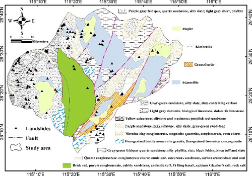
The Xing Guo area is located in the south of Jiangxi Province and lies between latitude 26°4′N and 26°42′N, and longitude 115°1′E and 116°51′E. It covers an area of approximately 3,215 km² (Figure 1). The altitude of the area ranges from 109 to 1,196 m above mean sea level. The slope angle of the study area varies between 0° to 67.5°. More than 43 geologic groups and units are recognized in this area (Table 1). The main lithology of the study area consists of purple grey feldspar, quartz sandstone, silty slate, light grey chert, and phyllite (Figure 2).

Figure 1. Landslide location map of the Xing Guo area (China map come from National Geographic World Map [ESRI 2010]).

Table 1. Types of geological formation of the Xing Guo area.

Class	Main lithology	Geology group and unit
A	Grey-green sandstone, silty slate, slate containing carbon	Ba cun group, Gao tan group
B	Quartz conglomerate, conglomerate coarse sandstone, calcareous sandstone, carbonaceous shale and coal	Zi shan group, Yun shan group, San mentang group, Zhang dong group
	Light grey dolomite, biological limestone, dolomitic limestone	Hu tian group, Da pu group, Ma ping group
C	Purple sandstone, pink siltstone, silty shale, grey-green sandstone	Zhong peng group, Xia shan group, Yun shan group
	Yellow calcareous siltstone and mudstone; purplish red sandstone	Zi shan group, San meng tang group, Zhang dong group
D	Kimberlite	Lu jin unit
E	Granodiorite	Xin quan unit
	Adamellite	Gu yinzhai unit, Huang po unit, Xiao bu unit, Yuan xiao unit
	Adamellite, Granodiorite	Ge xianshan unit, Ken qian unit, Yue xin unit, Heng shan unit, Ma zijian unit
F	Brick red, purple conglomerate, pebbly sandstone, andesitic tuff, Yi Ding basalt, calcium Glauber's salt, rock salt	Gui feng group, Tang bian group, He kou group, Ganzhou group, Mao dian group
G	Moraine clay conglomerate, magnetite quartzite, conglomerate, even cherts	Yan jiaqiao group
H	Grey-green feldspar quartz sandstone, silty phyllite, slate black folder; Shen tuff and slate	Tang tou group, Hu lin group, Shen shan group
I	Fine-grained biotite monzonite granite, fine-grained two-mica monzogranite	Qiao tou unit, Qing xi unit, Fu cheng unit,Tu qiao unit
J	Purple grey feldspar, quartz sandstone, silty slate; light grey chert, phyllite	Le changxia group, Ba li group, Lao hutang group, Gui keng unit

Figure 2. Geologic map of the study area.

The land-use map of the area was classified into six categories, namely, bare, forest, grass, water, farmland, and residential. Forest occupies the largest area (54.5%), whereas residential occupies 22.3%. Grass with farmland almost covers the same area (9.0%), and water covers 4.4%. Only 0.5% land-use area is bare.

The study area is located in a subtropical monsoon climate region. According to the Jiangxi Province Meteorological Bureau (http://www.weather.org.cn), the average annual rainfall in the Xing Guo weather station for 1960–2012 is from 895.3 mm (1963) to 2284.5 mm (1997). The total number of precipitation days is 156, and the rainy season is mainly from March to August, which accounts nearly 73.1% of the annual rainfall. In May and June, the average rainfall varies between 240 and 250 mm per month. The average annual temperature is 18.8 °C. The average annual evaporation is 1 635.8 mm, and the average relative humidity is 78%.

According to the Xing Guo County government, a total of 3,653 people in the study area are affected by the landslides (Hong et al. 2015). The estimated damages to properties are approximately US$4 million. However, in the study area not much preventive measures have been carried out to predict the location of landslides and prevent the damages caused by them. Therefore, analysing landslides in this area is crucial. The main factor that causes landslides in the Xing Guo area is the high amount of rainfall.

3. Data

3.1. Landslide inventory map

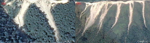
The landslide inventory map consisted of 79 landslide locations which was obtained from the Department of Land and Resources (http://www.jxgtt.gov.cn/) and the Meteorological Bureau of the Jiangxi Province (http://www.weather.org.cn/). The landslide inventory data was prepared by the aforementioned agencies through various means such as multiple field survey, and interpretation of 10-m resolution Google Earth images with a zoom-in and zoom out tools. Figure 3 shows some examples of landslides from Google Earth images.

Figure 3. Google Earth images of typical landslides.

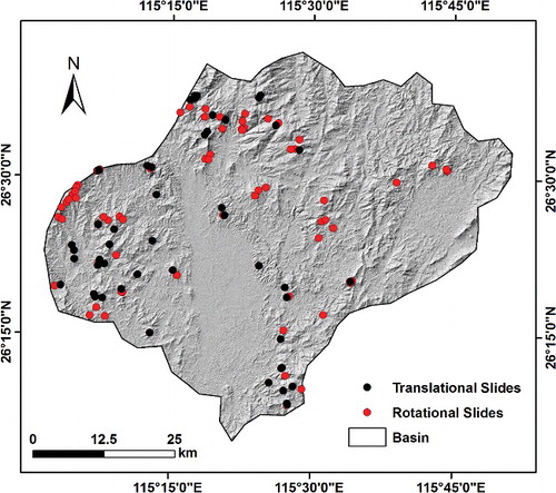
The landslide movement in the study area is mainly categorized into two types, translational slides (49) and rotational slides (79) (Figure 4). As different types of landslides have different occurrence mechanisms, thus they are required to be studied separately for better assessment. Therefore, this study focused on modelling rotational landslides, as there were more data available (79 compared to 49) where better assessment and comparison could be done.

Figure 4. Landslide inventory map.

To calculate the volume of landslides, the thickness and headscarp area were used from the digital elevation model (DEM). Then, the volume of a landslide ($V_s$) was calcuated as a wedge geometry model using the following equation (McAdoo et al. 2000):(1) $V_s=\frac{1}{2} \left(A_s\right)(h.\cos \left(\alpha \right),$(1) where $A_s$ is the area of landslide headscarp (m²), $h$ is the height of headscarp (m), and $\alpha$ is the scar slope angle in degrees. The volume of the smallest landslide is 30 m³, the largest is 60,000 m³, and the average is 874.2 m³. Large-volumed landslides (>1000 m³) occurred in the study area and affected 831 people. These landslides accounted for only 10.5% of the total number of landslides. Around 46.5% of the landslides are medium-volumed (200–1000 m³) and affected 1,066 people. Small-volumed landslides (<200 m³) affected 851 people accounting for 42.8% of the total landslides. The spatial distribution of the landslide locations along with their types is shown in Figure 4.

The dates of landslide occurrences are almost unknown. Thus, based on a random process, the landslide inventory data (79 landslides) was partitioned into two subsets (70/30). The first subset includes 55 landslide locations which are then used as training dataset, whereas the remaining 24 landslide locations were used as validation dataset.

3.2. Landslide conditioning factors

Overall, 16 landslide conditioning factors were analysed in this study area, such as slope, aspect, altitude, TWI, SPI, STI, soil, lithology, Normalized Difference Vegetation Index (NDVI), land use, rainfall, distance to road, distance to river, distance to fault, plan curvature, and profile curvature. Chi-square method was employed to compare the significance of each factor with landslide occurrence.

A DEM for the study area was acquired from the ASTER Gdem (http://gdem.ersdac.jspacesystems.or.jp/) at a scale of 30 m. Using this DEM, slope, altitude, aspect, plan curvature, profile curvature, streams, TWI, SPI, and STI were extracted in ArcGIS 10.2.

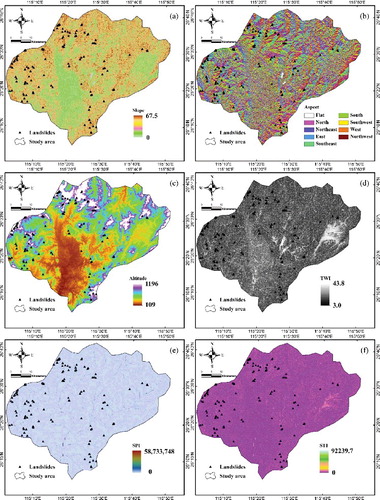
The slope angles were from 0° to 67.5° (Figure 5a). Slope angle is an important indicator in landslide formation because of its relationship with the gravitational force (Chen et al. 2017e). In general, the potential likelihood for landslides to occur increases with increasing of the slope angle. However, some favourable conditions are necessary. The aspect map (Figure 5b) was produced into nine classes, flat (−1), north (337.5°–360°, 0°–22.5°), northeast (22.5°–67.5°), east (67.5°–112.5°), southeast (112.5°–157.5°), south (157.5°–202.5°), southwest (202.5°–247.5°), west (247.5°–292.5°), and northwest (292.5°–337.5°). The direction of a slope face can affect the physical and biotic features of the slope and can significantly influence the local climate (microclimate). In some regions, patterns of soil differences related to differences exist. Thus, slope aspect indirectly affects the landslides (Pourghasemi et al. 2012; Jebur et al. 2014; Wen et al. 2016). The altitude map varied between 109 and 1196 m (Figure 5c). TWI is the major factor used to quantify the topographic control on hydrological processes, and it is a function of both the slope and flow direction. The formula of TWI is given as(2) $TWI = \text{ln}\left(\frac{A_s}{\beta }\right)$(2) where $A_s$ is the specific catchment area (m²/m) and$\beta$ is slope angle in degrees. The TWI map in this study was from 3.0 to 43.8 (Figure 5d). Stream power index (SPI) is the rate of energy at which water flows. SPI is defined as the movement of solid particles, typically because of a combination of gravity acting on the sediments. The formula of SPI is given as(3) $SPI =A_s \times \mathrm{ tan}\beta$(3) where $A_s$ is the specific catchment area (m²/m) and$\beta$ is slope angle in degrees.

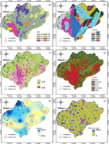
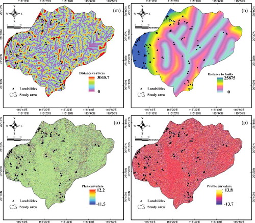
Figure 5. (a) Slope; (b) aspect; (c) altitude; (d) topographic wetness index (TWI); (e) stream power index (SPI); (f) sediment transport index (STI); (g) soil; (h) lithology; (i) NDVI; (j) land use; (k) rainfall; (l) distance to roads; (m) distance to rivers; (n) distance to faults; (o) plan curvature; (p) profile curvature.

On the other hand, STI explains the procedure of slope failure and deposition (Jebur et al. 2014). The formula of STI is as follows:(4) $STI ={\left(\frac{A_s}{22.13}\right)}^{0.6} \times {\left(\frac{\sin \beta }{0.0896}\right)}^{1.3}$(4) where $A_s$ is the specific catchment area (m²/m) and$\beta$ is slope angle in degrees.

Equation (4)(4) $STI ={\left(\frac{A_s}{22.13}\right)}^{0.6} \times {\left(\frac{\sin \beta }{0.0896}\right)}^{1.3}$(4) shows that the sediment transportation is controlled by the catchment area and slope angle. In general, the larger STI, the more water accumulates at the bottom of the catchment which then causes erosion.

The SPI and STI values ranged between 0 to 58,733,748 and 0–92,239.7, respectively (Figure 5e,f). The soil map was constructed into eight groups, namely, Ach, ACu, Alh, Atc, CMd, CMo, RGd, and WR (Figure 5g). The soil map was prepared in 1995 by the Institute of Soil Science, Chinese Academy of Sciences (http://www.issas.ac.cn/). Figure 1 shows the geological map of the study area at a scale of 1:200,000. The lithology map was obtained from China Geology Survey (http://www.cgs.gov.cn/) (see Table 1). The lithology map (Figure 5h) was constructed into eight groups (A, B, C, D, E, F, G, H, I, and J). The NDVI values varied between −0.48 and 0.56 (Figure 5i). The map was obtained from the Landsat 7 ETM⁺ satellite images, which were acquired on 10 December 1999. These images were obtained from the US Geological Survey (http://landsat.usgs.gov/).

Human activity plays an important role in changing land use in recent years. Land use is a human activity that significantly affects natural resources, soil, and plants. The land-use map was produced based on Landsat 7 ETM⁺ satellite images. Overall, six classes were recognized, namely, water, residential area, forest land, bare land, farmland, and grassland. The land-use map was produced using the Maximum likelihood supervised method with an accuracy of 92.5% (Figure 5j). The mean annual precipitation data were collected from the 29 rainfall stations were subsequently used to create the rainfall map (Figure 5k). A simple IDW (inverse distance weighted) interpolation method was used to produce the rainfall map. The precipitation data were extracted from a database from the government of Jiangxi Province Meteorological Bureau (http://www.weather.org.cn). Road and river networks were constructed into five group categories that undercut slopes larger than 15°, and were extracted from the topographic map at a scale of 1:50,000. Subsequently, the distance to road maps (Figure 5l) and the distance to river maps (Figure 5m) were prepared. The fault lines were extracted from the geological map at a scale of 1:200,000 and were employed to construct the distance to faults map. The value ranged from 0 to 25,875 m (Figure 5n). Furthermore, the plan and profile curvatures were extracted from the DEM and classified into three classes, flat, convex and concave (Figure 5o,p). The plan curvature which is created by intersecting a horizontal plane with the surface controls the divergence and convergence of water during the slides flow. On the other hand, the profile curvature is constructed by considering a profile parallel to the direction of the maximum slope. The profile curvature causes the acceleration or deceleration of water flow on the surface.

To assemble the conditioning factor maps and landslide inventory, the vector datasets were converted into raster data format with the reference scale of DEM (30 m). Finally, the factor maps and the landslide inventory data were combined to construct the matrix to develop the regression models in statistical software. The rows of the matrix contained the attributes of the predictor maps, whereas the columns represented the landslide and non-landslide samples. Aspect, soil, lithology, and land-use data were used as categorical variables whereas the remaining variables were used as continuous. To avoid the sensitivity of the models to the reclassification procedure of the continuous variables, they were not further reclassified into subclasses.

4. Method

4.1. Overall Flowchart

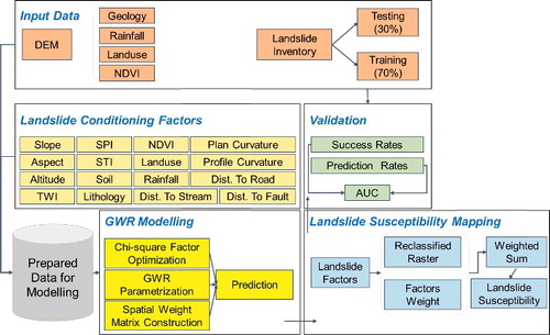
Figure 6 shows the overall GWR modelling workflow implemented in ArcGIS software. First, the necessary input data was gathered and managed in a proper data storage location. Then, 16 landslide conditioning factors were derived from various sources and by different methods. The details are explained in Section 3.2. In the GWR modelling stage, three main steps were applied. To optimize the landslide conditioning factors and selection, a chi-square factor optimization method was adopted. Then, by using an empirical analysis, the parameters of the GWR model were selected based on the training dataset, i.e. 30% of the whole landslide inventory data. Then, the spatial weight matrix was constructed using the optimized landslide conditioning factors and the landslide locations. Finally, the developed GWR regression model was applied to predict the probability of landslide occurrence in the remaining pixels locations in the dataset. The pixels that had values close to 1, interpreted as a high probability, whereas the pixels with values close to 0 interpreted as the low probability of landslide occurrence. Next, the landslide susceptibility was mapped by using the weighted sum function of ArcGIS. In this step, the estimated weight of each factor was used to overlay the landslide conditioning factors producing the landslide susceptibility index. Then, the landslide susceptibility index was converted into a probability by re-scaling into the range of 0–1 by using a linear function. After that, the probability raster map was reclassified into five classes of landslide susceptibility by the quantile classification approach. Finally, the landslide susceptibility map was validated by calculating the success and prediction rates using the testing dataset.

Figure 6. Overall workflow of GWR modelling for landslide susceptibility mapping.

4.2. Factor optimization – chi-square method

To evaluate the performance of different types of models, the quality of input data should be as high as possible to reach an accurate and reliable conclusion (Julong 1989; Breiman 2001; Wang 2005). The quality assessment for input data is essential because of the difficulty in preparing the landslide inventory map. Selecting significant parameters (landslide predictors) is another important step prior to landslide susceptibility modelling (Moh'd A Mesleh 2007). In this study, chi-square based factor optimization method was adopted to select significant landslide predictors for modelling purpose (Lineback Gritzner et al. 2001).

Pearson chi-square is the main test used to determine the significance of the relationship between different categorical variables (Satorra and Bentler 2001; Ye and Chen 2001). Its concept is based on computing the expected frequencies in a two-way table (i.e. no relationship exists between the variables) (Press 1966). The value of the chi-square and its significance level depend on the overall number of observations and the number of cells in the table (Regmi et al. 2010; Bryant and Satorra 2012). To calculate the importance of landslide predictors using chi-square method, the null hypothesis was defined first. The null hypothesis states that knowing the level of a landslide predictor does not help predict landslide occurrence (Sarkar and Kanungo 2004). The variables are independent.

H0:

Variable $X$ (e.g. slope) and variable $Y$ (e.g. landslide occurrence) are independent.

H1:

Variable $X$ (e.g. slope) and variable $Y$ (e.g. landslide occurance) are not independent:(5) ${\mathrm{\chi }}^2=\sum _{i=1}^n\frac{{\left(O_i-E_i\right)}^2}{E_i}$(5)

where $O_i$ is the observed frequency count at level $i$ of variable $X$ and $E_i$ is the expected frequency count at level $i$ of Variable $X$.

After the calculating the chi-square statistical value and the P-value for each predictor variable, the P-value was evaluated against the significance level (0.05) to estimate the relationship between the landslide predictor and landslide occurrence. A high chi-square value implies a high indicator performance to identify the landslides.

4.3. GWR

GWR is a spatial regression technique, which is widely used in geography and other disciplines (Brunsdon et al. 1996; Fotheringham et al. 1998; Brunsdon et al. 1999). Regression parameters in different geographic locations tend to exhibit various results (Leung et al. 2000; Brunsdon et al. 2001). The regression parameters are consistent with the changes of geographical positions (Atkinson et al. 2003; Song et al. 2014; Song et al. 2016). In utilizing the global spatial regression model, regression parameter estimation will be the regression parameters in the entire study area; the average value cannot reflect the regression parameters of the real feature space (Blanco-Moreno et al. 2008; Griffith 2008; Pirdavani et al. 2014b). Therefore, a model must be identified to deal with this problem.

In simple linear regression, the dependent variable is modelled as a linear function of a set of independent or influential variables as follows:(6) $y_i{\hspace{0.17em}=a}_0+\sum _{k = 1,m}{a}_k{x}_{ik}+{ϵ}_i i=\mathrm{1,2},\dots ,n$(6) where $y_i$is the $i$th observation of the dependent variable, $x_{ik}$ is the $i$th observation of the $k$th independent variable, the ${ϵ}_i$ is independent normally distributed errors terms with zero means, and each $a_k$ must be determined from a sample of $n$ observations (Brunsdon et al. 1996; Pirdavani et al. 2014a).

GWR is a relatively simple technique that extends the traditional regression framework of the equation by allowing local variations in the rates of change. Thus, the coefficients in the model are specific to a location $i$ instead of being global estimates. The regression equation is calculated as(7) $y_i{\hspace{0.17em}=a}_{i0}+\sum _{k = 1,m}{a}_{ik}{x}_{ik}+{ϵ}_i i=\mathrm{1,2},\dots ,n$(7) where $a_{ik}$ is the value of the $k$th parameter at location $i$. Equation (7)(7) $y_i{\hspace{0.17em}=a}_{i0}+\sum _{k = 1,m}{a}_{ik}{x}_{ik}+{ϵ}_i i=\mathrm{1,2},\dots ,n$(7) is a special case of Equation (6)(6) $y_i{\hspace{0.17em}=a}_0+\sum _{k = 1,m}{a}_k{x}_{ik}+{ϵ}_i i=\mathrm{1,2},\dots ,n$(6) where all the functions are constants across space. Point $i$, at which estimates of the parameters are obtained, is completely generalizable and not only needs points at which data are collected (Brunsdon et al. 1996; Lukawska-Matuszewska and Urbanski 2014).

The GWR produces localized versions of all standard regression diagnostics, including goodness-of-fit measures, such as $R^2$, and produces localized parameter estimates. The localized parameter estimates is useful for understanding the application of the model being calibrated and exploring the possibility of adding additional predictors to the model (Fotheringham et al. 1998).

In this sense, the difference between GWR and the spatial error approach is that spatial drift from ‘average’ global relationships is measured directly in the former, whereas it is measured as a second-order effect through the spatial distribution of residuals in the latter (Kimsey et al. 2008; Spurna 2008). The GWR is also used to improve our understanding of the processes being modelled, and thus separate local spatial anomalies in terms of each predictor (Brunsdon et al. 1999; Wei and Qi 2012).

The main idea of GWR is a spatial weight matrix; the result of GWR is influenced by selecting different spatial weighting functions ( Spurna 2008; Ogneva-Himmelberger et al. 2009). Regardless of the specific weighting function employed, the essential idea of GWR is that for each point $i$, a “bump of influence” exists around $i$ corresponding to the weighting function in such a way that sampled observations near to $i$ have more influence in the estimation of $i$'s parameters than that of sampled observations that are farther away (Brunsdon et al. 1996).

The main function of GWR is as follows:

4.3.1. Distance threshold function

Distance threshold function is the simplest and widely used method of the spatial weighting function and is expressed as(8) $W_{ij}=\left\{\begin{array}{l}1, d_{ij}<D\\ 0, d_{ij}>D\end{array}\right.$(8) where $D$ is the distance threshold and $d_{ij}$ is distance from return point $i$ to data point $j$.

4.3.2. Gaussian function

The essential idea of Gaussian function is to select a continuous monotonically decreasing function to express the relationship between $W_{ij}$ and $d_{ij}$ as (9) $W_{ij}= \text{exp}\left(-{\left(d_{ij}/b\right)}^2\right)$(9) where $b$ is defined as the bandwidth. If $i$ and$j$ coincide, the weight of data at that point will be combined and the weight of other data will decline according to a Gaussian curve as the distance between $i$ and $j$ increases (Fotheringham et al. 1998; Kumar et al. 2012).

4.3.3. Bisquare function

Equations (8)(8) $W_{ij}=\left\{\begin{array}{l}1, d_{ij}<D\\ 0, d_{ij}>D\end{array}\right.$(8) and (9(9) $W_{ij}= \text{exp}\left(-{\left(d_{ij}/b\right)}^2\right)$(9) ) can reach to a compromise solution which have a desirable property of excluding all data points greater than some distance from, as well as the analytically desirable property of continuity. An example of the bisquare function is given as(10) $W_{ij}=\left\{\begin{array}{l}{\left[1-{\left(d_{ij}/b\right)}^2\right]}^2, d_{ij}\le b\\ 0, { d}_{ij}>b\end{array}\right.$(10)

Equation (10)(10) $W_{ij}=\left\{\begin{array}{l}{\left[1-{\left(d_{ij}/b\right)}^2\right]}^2, d_{ij}\le b\\ 0, { d}_{ij}>b\end{array}\right.$(10) excludes points outside radius $d$ but tapers the weighting of points inside the radius. Thus, $W_{ij}$ is a continuous and once differentiable function for all points less than d units from $i$ (Zhang and Mei 2011; Chen et al. 2012).

Many previous works discussed the application of GWR (Harris et al. 2010; Koutsias et al. 2010; Paez et al. 2011; Zhang et al. 2011). To address the limit of the least square sum of squares, CV approach was suggested for local regression (Cleveland 1979) and is given as(11) $CV =\frac{1}{n} \sum _{i = 1}^n{\left[y_i-{\widehat{y}}_{\ne i}\left(b\right)\right]}^2$(11) where ${\widehat{y}}_{\ne i}\left(b\right)$ is the fitted value of $y_i$ with the observations for point $i$ omitted from the calibration process. This approach can counteract the ‘wrap-around’ effect because when $b$ becomes very small, the model is then calibrated on samples near $i$ and not at $i$ itself.

4.4. Stochastic gradient descent – log loss (logistic regression)

Stochastic gradient descent (SGD) is a stochastic solution of the gradient descent optimization for minimizing an objective function which is in a form of a sum of differentiable functions (Cleveland 1979; Langford et al. 2009; Bottou 2010; Bach 2014). One can generalize the loss function using Equation (12)(12) $J \left(w\right)=\sum _{i}L\left(m_i\left(w\right)\right)+\lambda R\left(w\right)$(12) . The loss function consists of two parts, namely, loss term and a regularization term. These two terms can be written as follows:(12) $J \left(w\right)=\sum _{i}L\left(m_i\left(w\right)\right)+\lambda R\left(w\right)$(12) (13) $m_i=y^{\left(i\right)} f_w\left(x^{\left(i\right)}\right)$(13) (14) $y^{\left(i\right)}\in \left\{-\mathrm{1,1}\right\}$(14) (15) $f_w \left(x^{\left(i\right)}\right)=w^T x^{\left(i\right)}$(15)

The log loss equivalent to the cross entropy loss function is used to train an LR model:(16) $J(w)=\hspace{0.17em}\lambda \Vert w{\Vert }^2+{\displaystyle \sum }_i{y}^i\log g_w(x^{\left(i\right)})+(1-y^i)(\log 1-g(x^{(i)})), y^{(i)}\in \{0,1\}$(16) $g_w \left(x^{\left(i\right)}\right)=\frac{1}{1+e^{-f_w\left(x^{\left(i\right)}\right)}}$$f_w \left(x^{\left(i\right)}\right)=w^T x^{\left(i\right)}$$1-g \left(x^{\left(i\right)}\right)=\frac{1}{1+e^{-f_w\left(x^{\left(i\right)}\right)}}$Thus, Equation (17)(16) $J(w)=\hspace{0.17em}\lambda \Vert w{\Vert }^2+{\displaystyle \sum }_i{y}^i\log g_w(x^{\left(i\right)})+(1-y^i)(\log 1-g(x^{(i)})), y^{(i)}\in \{0,1\}$(16) can be written as(17) $J(w)=\Vert w{\Vert }^2+{\displaystyle {\sum }_i\log 1+e^{-y^{\overline{(i)}}}{f}_w(x^{(i)})}$(17) $L \left(m\right)=\log 1 +e^{-m}$$m^i=y^{\stackrel{-}{\left(i\right)}} +f_w\left(x^{\left(i\right)}\right)$$y^{\stackrel{-}{\left(i\right)}}=\left\{\begin{array}{l}-1 if y^{\left(i\right)}=0 \\ 1 if y^{\left(i\right)}=1 \end{array}\right.$

4.5. Stochastic gradient descent – hinge loss (SVM)

The loss term for soft margin SVM is presented below (Bottou 2010). We use $L_{\mathrm{hinge}}$ to represent the hinge loss:(18) $J(w)=\frac{1}{2} \Vert w{\Vert }^2+{\displaystyle \sum }_i\max (0,1-y^i{w}^t{x}^i)$(18) (19) $=\frac{1}{2}{\Vert w\Vert }^2+{\displaystyle \sum }_i\max (0,1-m_i(w))$(19) (20) $=R_2 \left(w\right)+\sum _i{L}_{\mathrm{hinge}}\left(m_i\right).$(20)

4.6. Support vector machine

SVM is essentially a nonlinear data processing method that differs from neural networks. The former is based on structure risk minimization principle, whereas the latter is based on empirical risk minimization principle (Hong et al. 2015). These novel structure risk minimization principles are based on firm mathematical foundations and produce profound changes in understanding machine learning (Jebur et al. 2015). SVM has the following characteristics (Ren et al. 2015; Shahabi et al. 2015):

(1)	Simple structure.
(2)	Convex optimization, no local minimum.
(3)	Sparse representation: The direction of the optimal separating super-plane is a linear combination of training samples. The coefficient that is contained in each sample reflects its importance. All the information about classification is contained in support vectors whose coefficients are not zero. If non-support vectors are removed or shifted slightly, re-training leads to the same solution as before. In other words, the solution only depends on support vectors.
(4)	Modularization: SVM is composed of two modules, namely, a general-purpose learning machine and a domain-specific kernel function. Thus, we can design learning algorithm and kernel function in a modular way. This process is crucial for theoretical analysis and engineering implementation.

The most common formula of SVM classification is given as(21) $\mathrm{g }\left(x\right)=\mathrm{ sign}\left(\sum _{i = 1}^n{y}_i{a}_{i}K\left(x_i,y_i\right)+b\right)$(21) where $n$ denotes the number of training data points. Moreover, $x_i$ and $y_i$ are training and testing pattern, respectively. $b$ represents the bias term, and $K\left(x_i,y_i\right)$ is the kernel function.

In general, four types of kernels are used with SVM classifier, radial basis function (RBF), polynomial (PL), sigmoid (SIG), and linear (LN). In this research, the RBF kernel was selected because of the most common kernel function used in landslide susceptibility mapping and because it is less sensitive to outliers (Yao et al. 2008). The mathematical representation of RBF is shown as(22) $\text{Radial}\text{basis}\text{function}:K(x_i,y_i)=(-\gamma \Vert X_i-X_j\Vert ),\gamma >0,$(22) where $K\left(x_i,y_i\right)$ is the kernel function,$\gamma$ is the gamma term in the kernel function for all kernel types except linear, $d$ is the polynomial degree term in the kernel function for the polynomial kernel, $r$ is the bias term in the kernel function for the polynomial and sigmoid kernels, and $\gamma$, $d$, and $r$ are user-defined parameters; the correct definition of these parameters can increase the accuracy of the SVM solution (Su et al. 2015; Tehrany et al. 2015; Chen et al. 2016; Hong et al. 2016). Many previous works applied SVM methods in landslide susceptibility modelling (Chen et al. 2016; Hong et al. 2016).

4.7. Statistical evaluation measures

In this study, statistical index-based evaluations and receiver-operating characteristic (ROC) curve have been used to validate the produced landslide susceptibility maps. Statistical indexes such as sensitivity and specificity were used (Su et al. 2015; Chen et al. 2016, 2017g, 2017h). These metrics were calculated based on the confusion matrices resulting from the GWR, SGD-LR, SGD-SVM, and SVM models and the landslide inventory map:(23) $\mathrm{Sensitivity}=\frac{TP}{TP+FN}$(23) $1-\mathrm{specificity }=\frac{FP}{FP+TN}$where TP is the number of landslide points correctly classified to the landslide class and TN is the total number of non-landslide points correctly classified to the non-landslide class. FN is the number of landslide points classified to the non-landslide class, and FP is the non-landslide points classified to the landslide class (Frattini et al. 2010; Hong et al. 2016; Chen et al. 2017i).

On the other hand, the ROC curve which is a standard method to validate the general performance of landslide susceptibility models were constructed by plotting sensitivity and 100-specificity indexes (Pham et al. 2016). The area under the ROC curve was calculated to validate quantitatively the general performance of the landslide susceptibility models. The higher the AUC value, the better performance of landslide models. The performance of landslide models is perfect when the AUC is equal to 1.0 (Tien Bui et al. 2017b; Chen et al. 2017d). In addition, success curve rates and prediction curve rates were constructed using the landslide training and validation datasets, respectively. The success curve rate shows the performance of a landslide model to fit the training dataset, whereas the prediction curve rate depicts the performance of landslide models to predict landslides in unsampled areas.

Validation of landslide susceptibility maps is an important task that should be conducted to confirm the usability of the final maps using all kind of models. In the current study, landslide susceptibility maps produced by the four models were validated by comparing the susceptibility map with the training and the testing data. To conduct this process, 79 landslides were randomly separated into two datasets; 55 (70%) landslides were selected as the training data and the remaining 24 (30%) landslides were used as testing data.

5. Result

5.1. Results of chi-square factor optimization

Figure 7 shows the results of the chi-square test on the observed distribution and the expected distribution of the landslide occurrence based on posterior probabilities calculated using the 16 variables. The highest chi-square value (119.13) was observed for the slope factor indicating the high contribution of this factor to the rotational landslide occurrence in the study area. In addition, the chi-square values of the altitude, STI, distance to river, and aspect factors are greater than 60. However, the factors distance to road, plan curvature, NDVI, and land use had relatively low chi-square values below 10.

Figure 7. Chi-square importance of landslide conditioning factors.

To select the best subset of landslide conditioning factors, a threshold of the chi-square value must be established. No standard methods were developed to select these thresholds because these methods depend on the characteristics of the study area and datasets used. Therefore, the factor subset selection depends on the analyst. In our case, three experiments with best 5, 10, and 15 factors were conducted to select the best subset for GWR modelling. The success and prediction rates of the four models (SVM, SGD-SVM, SGD-LR, GWR) using the three-factor subsets are shown in Table 2. In general, the results demonstrated that a larger number of landslide conditioning factors obtain a higher prediction accuracy except with SGD-LR model. The best accuracies of SVM, SGD-SVM, and GWR were obtained with using 15 factors. On the other hand, the highest accuracy of SGD-LR was obtained with 10 factors. Increasing the number of factors from 10 to 15 affects the accuracy of the SVM, SGD-SVM, and GWR models. The prediction accuracy of GWR was increased from 0.83 to 0.85 when the number of factors increased from 10 to 15. Therefore, considering the focus of this paper (i.e. GWR modelling) the 15 factors were used to produce the landslide susceptibility maps for the study area.

Table 2. The success and prediction rates of the four models with 5, 10, and 15 landslide conditioning factors.

	SVM		SGD-SVM		SGD-LR		GWR
Experiment	Success rate	Prediction rate	Success rate	Prediction rate	Success Rate	Prediction rate	Success Rate	Prediction rate
Best 5 factors	0.67	0.62	0.68	0.63	0.81	0.82	0.79	0.79
Best 10 factors	0.73	0.68	0.74	0.68	0.83	0.85	0.84	0.83
Best 15 factors	0.79	0.73	0.81	0.75	0.83	0.83	0.87	0.85

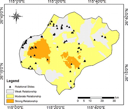
5.2. Results of spatial correlation among landslide locations in the study area

The estimation of parameter coefficients by GWR required the mapping of spatial correlation among landslide locations in the study area. The spatial correlations among landslide locations were calculated and represented by a spatial weight matrix. This matrix is a representation of the spatial structure of landslide data. The spatial weights matrix imposes a structure on the landslide data, which is crucial to select a conceptualization that best reflects how features actually interact with each other. In this study, the inverse distance was selected because it is most appropriate than other available methods in ArcMap 10.2. The spatial weight matrix is employed to generate the spatial correlation map of landslides in the study area.

Figure 8 shows the results of the spatial correlation among landslide locations in the study area. In a physical sense, the spatial weights indicate the variations of landslide locations in terms of spatial distribution. In other words, the geographical location is an important indicator for a landslide, and each landslide location was compared with the neighbouring landslides using the Euclidean distance. This process was important to ensure that landslides have influences according to their spatial distributions and relations to neighbour slides. The correlations were estimated as continuous values ranged from 0 to 1. However, these correlations are shown as categorical classes. Thus, the interpretation of the map becomes significantly easier. The spatial correlations were categorized into three classes, namely, weak relationship (0–0.6), moderate relationship (0.61–0.7), and strong relationship (0.71–1), by the quantile method. Few landslides in the study area were highly correlated. This result can be observed in the west and middle parts of the study area. However, most landslides exhibited weak and moderate spatial relationships, which can be seen in the east, south, and some parts in north of the study area. This map was used to generate landslide susceptibility by GWR method, which is presented in the next section.

Figure 8. Spatial correlation of landslide locations in the study area.

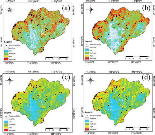
5.3. Landslide susceptibility modelling

Four landslide susceptibility maps were produced for the study area by employing GWR, SGD-LR, SGD-SVM, and SVM models (Figure 9). The first examination of the susceptibility maps shows that all the models agree that the northwest part of the study area is highly susceptible to rotational landslides. The maps show that the majority of the study area has low/moderate susceptibility to landslides. GWR and SGD-LR models produced maps where the high and very high susceptibility classes have larger areas compared with SVM models.

Figure 9. Landslide susceptibility maps: (a) GWR, (b) SGD-LR, (c) SGD-SVM, and (d) SVM.

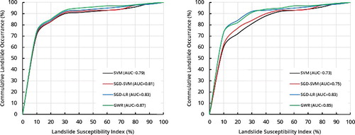
Using the 15 landslide conditioning factors, the SVM, SGD-SVM, SGD-LR and GWR models were constructed using the training data. The ROC curves and AUC values of the four models are presented in Figure 10. The GWR model exhibits the highest performance in terms of success rate and prediction rate with values of 0.87 and 0.85, respectively. The SGD-LR model exhibited slightly lower success and prediction rates (0.83) than GWR model. The SGD-SVM model showed better success and prediction rates than the normal SVM model. The success rates of SGD-SVM and SVM models were 0.81 and 0.79, respectively. In addition, the prediction rates of these models were slightly lower than success rates. Overall, the result of the validation of the four models indicates that GWR is a better model than other widely used models.

Figure 10. ROC curves. Success rate (left) and prediction rate (right).

Table 3 shows the estimated coefficient values for the landslide conditioning factors by the models developed in the current study. The coefficients were standardized using the expression presented in Equation (24)(24) $W_{s,i} \left(k\right)=\frac{W_i\left(k\right)-\min W_i\left(k\right)}{\max W_i\left(k\right)-\min W_i\left(k\right)}, k=\mathrm{1,2},\mathrm{3,4}$(24) . The result illustrates that the four landslide susceptibility models are consistent in terms of altitude, slope, NDVI, and aspect, which are the most important factors that contribute to landslides in the study area:(24) $W_{s,i} \left(k\right)=\frac{W_i\left(k\right)-\min W_i\left(k\right)}{\max W_i\left(k\right)-\min W_i\left(k\right)}, k=\mathrm{1,2},\mathrm{3,4}$(24) where $W_{s,i}\left(k\right)$is the standardized weight at kth approach,$W_i\left(k\right)$ is the calculated weight by the kth approach, and $i$ is the identity number of each parameters (e.g. $i$value of slope = 8).

Table 3. The estimated coefficient values for the landslide conditioning factors by the models developed in the current study.

	Weight value (standardized by Equation 1)
Factor	SVM	SGD-SVM	SGD-LR	GWR
Altitude	0.488	0.747	0.889	0.587
Aspect	0.319	0.461	0.498	0.296
Distance to fault	0.525	0.631	0.738	0.475
Land use	0.383	0.579	0.627	0.404
Lithology	0.224	0.448	0.456	0.246
NDVI	1.000	1.000	1.000	1.000
Plan curvature	0.118	0.000	0.000	0.000
TWI	0.309	0.359	0.334	0.239
STI	0.000	0.327	0.361	0.063
Soil	0.110	0.400	0.300	0.192
Slope	0.953	0.955	0.989	0.924
Distance to road	0.462	0.576	0.619	0.448
Distance to river	0.108	0.344	0.460	0.157
Rainfall	0.288	0.459	0.328	0.306
Profile curvature	0.419	0.517	0.481	0.413

6. Discussion

Producing accurate landslide susceptibility maps is difficult because of several reasons, such as soil condition, bedrock, topography, hydrology, and human activities. Therefore, the comparative study of landslide susceptibility models is progressing in the scientific literature. In this study, four models were assessed, namely, GWR, SGD-LR, SGD-SVM, and SVM. A total of 79 landslides and 16 conditioning factors, such as slope, aspect, altitude, TWI, SPI, STI, soil, lithology, NDVI, land use, rainfall, distance to road, distance to river, distance to fault, and plan curvature, profile curvature, were analysed. Only the significant factors were used in the susceptibility mapping.

6.1. Impact of landslide conditioning factors

In this study, the chi-square method was used to select significant landslide conditioning factors to be used in susceptibility models. This process can reduce over-fitting to the training data and speed up the classification process. In addition, non-significant factors may generate severe multicollinearity, which can disrupt regression estimates. Therefore, employing this technique was important in landslide mapping, which was conducted in the current study. The chi-square method evaluated landslide factors individually with respect to the presence or absence of landslides. The results revealed that SPI factor is not significant for landslide susceptibility modelling in the study area whereas slope and altitude were determined to be the most influential factors. In the generated regression models, the slope was given a high coefficient, which indicates its importance for the spatial prediction of landslides. However, plan curvature was given a relatively low coefficient by the four models. As a result, the interpretation of the estimated coefficients in the models cannot describe the importance of landslide factors by evaluating only one model. To explain the causes of landslides, several models should be analysed. This analysis is crucial to determine the important factors that cause landslides.

6.2. Prediction accuracy of the models

The comparative study of the four models showed that the prediction rate of the four models is quite close to each other. The highest prediction rate of (0.85) was achieved by the GWR model. The results also revealed that the SGD learning approach could improve the prediction accuracy of landslides in SVM models. The success and prediction rates of the traditional SVM were slightly lower than the SGD-SVM approach. In addition, according to the successive and predictive curve rates, the performance of SGD-LR is higher than SGD-SVM using the training dataset. The hyperparameters of the SVM model could be fine-tuned such that it could perform well on the training dataset. The predictive rate of SGD-SVM is lower than those of SGD-LR. This indicates that the global LR model has more generalization capability and less sensitive to over-fitting.

One of the main advantages of GWR is that it can integrate geographical location and other landslide conditioning factors for estimating the spatial distribution of landslides and reflects the non-stationary spatial relationship between these factors and landslide occurrence probability. The spatial variations exhibit in landslide conditioning factors within the study area is a challenge when using most of statistical and data mining methods. A factor can have either positive or negative effect on landslide occurrence in these methods. On the other hand, the GWR method generates local regression models that vary according to the geographic location in the study area. Compared with other traditional models, GWR achieved better accuracy and explained the spatial distribution characteristics of landslides in the study area. However, the results of the current study showed that the GWR model could achieve better accuracy with 15 factors compared to LR where it achieved the highest prediction accuracy with only 10 factors. Using a large number of factors in GWR modelling can yield to a severe multicollinearity problem where the GWR model cannot be efficiently built. Therefore, further improvements in factor optimization for GWR should be explored and deeply investigated. Another important point is the temporal correlation of landslides. With comprehensive landslide inventory data where the temporal information is available, the GWR model can be further enhanced to include spatial-temporal modelling for landslide susceptibility mapping. Furthermore, because GWR is a local regression method, the spatial resolution of the input data can have a significant effect on its accuracy and performance. Thus, the effects of the spatial resolution of input data on GWR modelling is recommended to be studied in future works.

6.3. Contribution of the study and results of previous studies

Comparative study of modelling methods is a classical research area in landslide susceptibility assessment. The main goal of these works is to understand the prediction capability of the models and the effect of their hyperparameters in different environments on different datasets. Even though the science in this field has progressed a lot, several models including GWR have not been fully understood in the context of landslide modelling. The contribution of this study is to understand the prediction accuracy of the GWR model and its sensitivity to the number of landslide conditioning factor in the case study of Xing Guo area (China).

As landslide occurrences and conditioning factors have spatial variations, global models such as neural network or LR ignore autocorrelation characteristics of data between the landslide locations in susceptibility modelling. In the literature, several studies have compared spatial regression and global models. Erener and Düzgün (2010) found that the spatial regression model which estimates the coefficients at local scale has better generalization performance (AUC = 0.83) than the LR model (AUC = 0.74). Feuillet et al. (2014) suggested that GWR-based modelling provides significant inputs for landslide susceptibility mapping, by highlighting local drivers, indecipherable in global models. More recently, Yu et al. (2016) developed a landslide susceptibility model utilizing the GWR approach and they found that their model outperforms the SVM model in terms of prediction capability by up to 19%. In addition, they indicated that the slope and distance from drainage are greatly significant for landslide occurrence in their study area. In our study, according to the coefficients estimated by the GWR, the slope and distance from the river are influential factors. Other studies such as by Park and Kim (2015) and Sabokbar et al. (2014) have shown that high prediction accuracy better than global LR model can be achieved by the GWR model for landslide susceptibility mapping.

7. Conclusion

In this paper, a comparative experiment between GWR, SVM, and LR for landslide susceptibility mapping is presented using multisource data of the Xing Guo area in China. The GWR model was developed using the significant factors selected by the chi-square method. Several subsets of landslide factors were analysed and the sensitivity of the GWR model to the number of the selected factors is reported. The results of the comparative study showed that the GWR outperforms the SVM and LR models in terms of prediction capability. Based on the results obtained from the current study, GWR can be used for the spatial prediction of landslides and it is comparable to the well-known methods (i.e. SVM and LR). The landslide susceptible zones represent an important base for assessing landslide hazard and risk over the study area. Consequently, the generated maps could be useful to local authorities and decision makers for selecting suitable locations for future land-use planning and implementation of development.

However, there are several points that need to be considered in future works as follows: (1) the GWR model was found to perform better when using 15 landslide factors compared with using less number of factors. In this context, other optimization methods (i.e. Random Forest, Ant Colony) should be investigated to attempt reducing the number of factors while preserving the prediction accuracy of the model. This can improve the general performance of the GWR model; reducing the multicollinearity problem and the sensitivity of the model to overfitting especially in data-scarce environments. The second point that needs to be addressed is the integration of the spatial regression models (e.g. GWR) with other statistical and data mining methods to improve the prediction capability of the landslide susceptibility models. Finally, with comprehensive landslide inventory data, both spatial and temporal autocorrelations can be investigated in the spatial regression model or in the integrated models.

Disclosure statement

No potential conflict of interest was reported by the authors.

Additional information

Funding

This work was supported by the National Natural Science Foundation of China [grant number 41472202], [grant number 41401032], CAS-VPST Silk Road Science Fund 2018 [grant number GJHZ1855] and General Programme of Jiangxi Meteorological Bureau.

References

- Atkinson PM, German SE, Sear DA, Clark MJ. 2003. Exploring the relations between riverbank erosion and geomorphological controls using geographically weighted logistic regression. Geogr Anal. 35:58–82.
- Bach F. 2014. Adaptivity of averaged stochastic gradient descent to local strong convexity for logistic regression. J Mach Learn Res. 15:595–627.
- Beyabanaki SAR, Bagtzoglou AC, Anagnostou EN. 2016. Effects of groundwater table position, soil strength properties and rainfall on instability of earthquake-triggered landslides. Environ Earth Sci. 75:1–13.
- Blanco-Moreno JM, Chamorro L, Izquierdo J, Masalles RM, Sans FX. 2008. Modelling within-field spatial variability of crop biomass – weed density relationships using geographically weighted regression. Weed Res. 48:512–522.
- Bottou L. 2010. Large-scale machine learning with stochastic gradient descent. Proceedings of COMPSTAT'2010. Paris: Springer. p. 177–186.
- Breiman L. 2001. Random forests. Mach Learn. 45:5–32.
- Brunsdon C, Fotheringham AS, Charlton M. 1999. Some notes on parametric significance tests for geographically weighted regression. J Regional Sci. 39:497–524.
- Brunsdon C, Fotheringham AS, Charlton ME. 1996. Geographically weighted regression: a method for exploring spatial nonstationarity. Geogr Anal. 28:281–298.
- Brunsdon C, McClatchey J, Unwin D. 2001. Spatial variations in the average rainfall–altitude relationship in Great Britain: an approach using geographically weighted regression. Int J Climatol. 21:455–466.
- Bryant FB, Satorra A. 2012. Principles and practice of scaled difference chi-square testing. Struct Equ Model. 19:372–398.
- Carlini M, et al. , 2016. Tectonic control on the development and distribution of large landslides in the Northern Apennines (Italy). Geomorphology. 253:425–437.
- Chen G, Zhao KG, McDermid GJ, Hay GJ. 2012. The influence of sampling density on geographically weighted regression: a case study using forest canopy height and optical data. Int J Remote Sens. 33:2909–2924.
- Chen W, Chai HC, Zhao Z, Wang QQ, Hong HY, 2016. Landslide susceptibility mapping based on GIS and support vector machine models for the Qianyang County, China. Environ Earth Sci, 75:474.
- Chen W, Panahi M, Pourghasemi HR. 2017a. Performance evaluation of GIS-based new ensemble data mining techniques of adaptive neuro-fuzzy inference system (ANFIS) with genetic algorithm (GA), differential evolution (DE), and particle swarm optimization (PSO) for landslide spatial modelling. Catena. 157:310–324.
- Chen W, Pourghasemi HR, Kornejady A, Zhang N. 2017b. Landslide spatial modeling: Introducing new ensembles of ANN, MaxEnt, and SVM machine learning techniques. Geoderma. 305:314–327.
- Chen W, Pourghasemi HR, Naghibi SA. 2017c. A comparative study of landslide susceptibility maps produced using support vector machine with different kernel functions and entropy data mining models in China. Bull Eng Geol Environ. 1–18.
- Chen W, Pourghasemi HR, Naghibi SA. 2017d. Prioritization of landslide conditioning factors and its spatial modeling in Shangnan County, China using GIS-based data mining algorithms. Bull Eng Geol Environ. 2017:1–19.
- Chen W, Pourghasemi HR, Panahi M, Kornejady A, Wang J, Xie X, Cao S. 2017e. Spatial prediction of landslide susceptibility using an adaptive neuro-fuzzy inference system combined with frequency ratio, generalized additive model, and support vector machine techniques. Geomorphology. 297:69–85.
- Chen W, Pourghasemi HR, Zhao Z. 2017f. A GIS-based comparative study of Dempster-Shafer, logistic regression and artificial neural network models for landslide susceptibility mapping. Geocarto Int. 32:367–385.
- Chen W, Shirzadi A, Shahabi H, Ahmad BB, Zhang S, Hong H, Zhang N. 2017g. A novel hybrid artificial intelligence approach based on the rotation forest ensemble and naïve Bayes tree classifiers for a landslide susceptibility assessment in Langao County, China. Geomat Nat Haz Risk. 1–23. https://doi.org/10.1080/19475705.2017.1401560
- Chen W, Xie X, Peng J, Wang J, Duan Z, Hong H. 2017h. GIS-based landslide susceptibility modelling: a comparative assessment of kernel logistic regression, Naïve-Bayes tree, and alternating decision tree models. Geomat Nat Haz Risk. 1–24. https://doi.org/10.1080/19475705.2017.1289250
- Chen W, Xie X, Wang J, Pradhan B, Hong H, Bui DT, Duan Z, Ma J. 2017i. A comparative study of logistic model tree, random forest, and classification and regression tree models for spatial prediction of landslide susceptibility. Catena. 151:147–160.
- Chou H-T, Lee C-F, Lo C-M. 2017. The formation and evolution of a coastal alluvial fan in eastern Taiwan caused by rainfall-induced landslides. Landslides. 14:109–122.
- Chung M-C, Tan C-H, Chen C-H. 2017. Local rainfall thresholds for forecasting landslide occurrence: Taipingshan landslide triggered by Typhoon Saola. Landslides. 14:19–33.
- Ciurleo M, Calvello M, Cascini L. 2016. Susceptibility zoning of shallow landslides in fine grained soils by statistical methods. Catena. 139:250–264.
- Cleveland WS. 1979. Robust locally weighted regression and smoothing scatterplots. J Am Statist Assoc. 74:829–836.
- Conte E, Donato A, Troncone A. 2017. A simplified method for predicting rainfall-induced mobility of active landslides. Landslides. 14:35–45.
- Dickson ME, Perry GLW. 2016. Identifying the controls on coastal cliff landslides using machine-learning approaches. Environ Model Software. 76:117–127.
- Erener A, Düzgün HSB. 2010. Improvement of statistical landslide susceptibility mapping by using spatial and global regression methods in the case of More and Romsdal (Norway). Landslides. 7:55–68.
- Fan L, Lehmann P, Or D. 2016. Effects of soil spatial variability at the hillslope and catchment scales on characteristics of rainfall-induced landslides. Water Resour Res. 52:1781–1799.
- Feng Z-y, Lo C-M, Lin Q-F. 2017. The characteristics of the seismic signals induced by landslides using a coupling of discrete element and finite difference methods. Landslides. 14:661–674.
- Feuillet T, Coquin J, Mercier D, Cossart E, Decaulne A, Jónsson HP, Sæmundsson Þ. 2014. Focusing on the spatial non-stationarity of landslide predisposing factors in northern Iceland: do paraglacial factors vary over space? Prog Phys Geog. 38:354–377.
- Fotheringham AS, Charlton ME, Brunsdon C. 1998. Geographically weighted regression: a natural evolution of the expansion method for spatial data analysis. Environ Plan A. 30:1905–1927.
- Franz M, Carrea D, Abellán A, Derron M-H, Jaboyedoff M. 2017. Use of targets to track 3D displacements in highly vegetated areas affected by landslides. Landslides. 13:821–831.
- Frattini P, Crosta G, Carrara A. 2010. Techniques for evaluating the performance of landslide susceptibility models. Eng Geol. 111:62–72.
- Griffith DA. 2008. Spatial-filtering-based contributions to a critique of geographically weighted regression (GWR). Environ Plan A. 40:2751–2769.
- Harris P, Fotheringham AS, Crespo R, Charlton M. 2010. The use of geographically weighted regression for spatial prediction: an evaluation of models using simulated data sets. Math Geosci. 42:657–680.
- Hong HY, et al. , 2016. Spatial prediction of landslide hazard at the Luxi area (China) using support vector machines. Environ Earth Sci. 75:40.
- Hong HY, Pradhan B, Xu C, Tien Bui D. 2015. Spatial prediction of landslide hazard at the Yihuang area (China) using two-class kernel logistic regression, alternating decision tree and support vector machines. Catena. 133:266–281.
- Hong HY, Chen W, Xu C, Youssef AM, Pradhan B, Tien Bui D. 2017a. Rainfall-induced landslide susceptibility assessment at the Chongren area (China) using frequency ratio, certainty factor, and index of entropy. Geocarto Int. 32:139–154.
- Hong HY, Ilia I, Tsangaratos P, Chen W, Xu C. 2017b. A hybrid fuzzy weight of evidence method in landslide susceptibility analysis on the Wuyuan area, China. Geomorphology. 290:1–16.
- Hong HY, Liu J, Zhu A-X, Shahabi H, Pham BT, Chen W, Pradhan B, Bui DT. 2017c. A novel hybrid integration model using support vector machines and random subspace for weather-triggered landslide susceptibility assessment in the Wuning area (China). Environ Earth Sci. 76:652.
- Hong HY, Pradhan B, Sameen MI, Kalantar B, Zhu A, Chen W. 2017d. Improving the accuracy of landslide susceptibility model using a novel region-partitioning approach. Landslides. 1–20.
- Jebur MN, Pradhan B, Tehrany MS. 2014. Optimization of landslide conditioning factors using very high-resolution airborne laser scanning (LiDAR) data at catchment scale. Remote Sens Environ. 152:150–165.
- Jebur MN, Pradhan B, Tehrany MS. 2015. Manifestation of LiDAR-Derived Parameters in the Spatial Prediction of Landslides Using Novel Ensemble Evidential Belief Functions and Support Vector Machine Models in GIS. IEEE J Sel Topics Appl Earth Observ Remote Sens. 8:674–690.
- Julong D. 1989. Introduction to grey system theory. J Grey Syst. 1:1–24.
- Kimsey MJ, Moore J, McDaniel P. 2008. A geographically weighted regression analysis of Douglas-fir site index in north central Idaho. Forest Sci. 54:356–366.
- Koutsias N, Martinez-Fernandez J, Allgower B. 2010. Do Factors Causing Wildfires Vary in Space? Evidence from Geographically Weighted Regression. Gisci Remote Sensing. 47:221–240.
- Kumar S, Lal R, Liu DS. 2012. A geographically weighted regression kriging approach for mapping soil organic carbon stock. Geoderma. 189:627–634.
- Langford J, Li L, Zhang T, 2009. Sparse online learning via truncated gradient. Advances in Neural Information Processing Systems 21 (NIPS 2008), pp. 905–912.
- Larsen IJ, Montgomery DR, Korup O. 2010. Landslide erosion controlled by hillslope material. Nat Geosci. 3(4):247–251.
- Lee C-F, Lo C-M, Chou H-T, Chi S-Y. 2015. Landscape evolution analysis of large scale landslides at Don-Ao Peak. Taiwan Environ Earth Sci. 75:1–19.
- Leung Y, Mei C-L, Zhang W-X. 2000. Testing for spatial autocorrelation among the residuals of the geographically weighted regression. Environ Plan A. 32:871–890.
- Lineback Gritzner M, Marcus WA, Aspinall R, Custer SG. 2001. Assessing landslide potential using GIS, soil wetness modeling and topographic attributes, Payette River, Idaho. Geomorphology. 37:149–165.
- Lukawska-Matuszewska K, Urbanski JA. 2014. Prediction of near-bottom water salinity in the Baltic Sea using Ordinary Least Squares and Geographically Weighted Regression models. Estuar Coast Shelf Sci. 149:255–263.
- McAdoo BG, Pratson LF, Orange DL. 2000. Submarine landslide geomorphology. US Cont slope Mar Geol. 169(1):103–136.
- Moh'd A Mesleh A. 2007. Chi square feature extraction based SVMs Arabic language text categorization system. J Comput Sci. 3:430–435.
- Ogneva-Himmelberger Y, Pearsall H, Rakshit R. 2009. Concrete evidence & geographically weighted regression: a regional analysis of wealth and the land cover in Massachusetts. Appl Geogr. 29:478–487.
- Osadchiev AA, Korotenko KA, Zavialov PO, Chiang WS, Liu CC. 2016. Transport and bottom accumulation of fine river sediments under typhoon conditions and associated submarine landslides: case study of the Peinan River, Taiwan Nat Hazards Earth Syst Sci. 16:41–54.
- Paez A, Farber S, Wheeler D. 2011. A simulation-based study of geographically weighted regression as a method for investigating spatially varying relationships. Environ Plan A. 43:2992–3010.
- Park S, Kim J. (2015). A comparative analysis of landslide susceptibility assessment by using global and spatial regression methods in Inje Area, Korea. Korean J Geomat. 33(6):579–587.
- Pham BT, Pradhan B, Bui DT, Prakash I, Dholakia MB. 2016. A comparative study of different machine learning methods for landslide susceptibility assessment: a case study of Uttarakhand area (India). Environ Model Software. 84:240–250.
- Pirdavani A, Bellemans T, Brijs T, Kochan B, Wets G. 2014a. Assessing the road safety impacts of a teleworking policy by means. of geographically weighted regression method. J Transp Geogr. 39:96–110.
- Pirdavani A, Bellemans T, Brijs T, Wets G. 2014b. Application of Geographically Weighted Regression Technique in Spatial Analysis of Fatal and Injury Crashes. J Transp Eng. 140:1–26.
- Pourghasemi HR, Mohammady M, Pradhan B. 2012. Landslide susceptibility mapping using index of entropy and conditional probability models in GIS: Safarood Basin, Iran. Catena. 97:71–84.
- Press SJ. 1966. Linear combinations of non-central chi-square variates. Ann Math Stat. 37:480–487.
- Promper C, Glade T. 2016. Multilayer-exposure maps as a basis for a regional vulnerability assessment for landslides: applied in Waidhofen/Ybbs, Austria. Nat Hazards. 82:111–127.
- Regmi NR, Giardino JR, Vitek JD. 2010. Modeling susceptibility to landslides using the weight of evidence approach: Western Colorado, USA. Geomorphology. 115:172–187.
- Ren F, Wu XL, Zhang KX, Niu RQ. 2015. Application of wavelet analysis and a particle swarm-optimized support vector machine to predict the displacement of the Shuping landslide in the Three Gorges, China. Environ Earth Sci. 73:4791–4804.
- Romano A, et al., 2016. Tsunamis generated by landslides at the coast of conical islands: experimental benchmark dataset for mathematical model validation. Landslides. 13:1379–1393.
- Sabokbar HF, Roodposhti MS, Tazik E. 2014. Landslide susceptibility mapping using geographically-weighted principal component analysis. Geomorphology. 226:15–24.
- Sarkar S, Kanungo DP. 2004. An integrated approach for landslide susceptibility mapping using remote sensing and GIS. Photogramm Eng Remote Sensing. 70(5):617–625.
- Satorra A, Bentler PM. 2001. A scaled difference chi-square test statistic for moment structure analysis. Psychometrika. 66:507–514.
- Shahabi H, Hashim M, Bin Ahmad B. 2015. Remote sensing and GIS-based landslide susceptibility mapping using frequency ratio, logistic regression, and fuzzy logic methods at the central Zab basin, Iran. Environ Earth Sci. 73:8647–8668.
- Shi JS, Wu LZ, Wu SR, Li B, Wang T, Xin P, 2016. Analysis of the causes of large-scale loess landslides in Baoji, China. Geomorphology. 264:109–117.
- Song WZ, Jia HF, Huang JF, Zhang YY. 2014. A satellite-based geographically weighted regression model for regional PM2.5 estimation over the Pearl River Delta region in China. Remote Sens Environ. 154:1–7.
- Song XD, Brus DJ, Liu F, Li DC, Zhao YG, Yang JL, Zhang GL, 2016. Mapping soil organic carbon content by geographically weighted regression: a case study in the Heihe River Basin, China Geoderma. 261:11–22.
- Spurna P. 2008. Geographically weighted regression: method for analysing spatial non-stationarity of geographical phenomenon. Geografie. 113:125–139.
- Su C, Wang LL, Wang XZ, Huang ZC, Zhang XC. 2015. Mapping of rainfall-induced landslide susceptibility in Wencheng, China, using support vector machine. Nat Hazards. 76:1759–1779.
- Tehrany MS, Pradhan B, Jebur MN. 2015. Flood susceptibility analysis and its verification using a novel ensemble support vector machine and frequency ratio method. Stoch Environ Res Risk Assess. 29:1149–1165.
- Tien Bui D et al., 2017a. Spatial prediction of rainfall-induced landslides for the Lao Cai area (Vietnam) using a hybrid intelligent approach of least squares support vector machines inference model and artificial bee colony optimization. Landslides. 14:447–458.
- Tien Bui D, Nguyen QP, Hoang N-D, Klempe H. 2017b. A novel fuzzy K-nearest neighbor inference model with differential evolution for spatial prediction of rainfall-induced shallow landslides in a tropical hilly area using GIS. Landslides. 14:1–17.
- Tien Bui D, Pham BT, Nguyen QP, Hoang N-D. 2016. Spatial prediction of rainfall-induced shallow landslides using hybrid integration approach of Least-Squares Support Vector Machines and differential evolution optimization: a case study in Central Vietnam. Int J Digital Earth. 9:1077–1097.
- Wang Y. 2005. Application of fuzzy decision optimum model in selecting supplier. J Sci Technol Eng. 5:1100–1103.
- Wang Y, Song C, Lin Q, Li J. 2016. Occurrence probability assessment of earthquake-triggered landslides with Newmark displacement values and logistic regression: The Wenchuan earthquake, China. Geomorphology. 258:108–119.
- Webster JM, George NPJ, Beaman RJ, Hill J, Puga-Bernabéu A, Hinestrosa G, Abbey EA, Daniell JJ. 2016. Submarine landslides on the Great Barrier Reef shelf edge and upper slope: a mechanism for generating tsunamis on the north-east Australian coast? Mar Geol. 371:120–129.
- Wei CH, Qi F. 2012. On the estimation and testing of mixed geographically weighted regression models. Econ Model. 29:2615–2620.
- Wen B-P, Jiang X-Z. 2016. Effect of gravel content on creep behavior of clayey soil at residual state: implication for its role in slow-moving landslides. Landslides. 1–18.
- Wen Z, He B, Xu D, Feng Q. 2016 November. A method for landslide susceptibility assessment integrating rough set and decision tree: A case study in Beichuan, China. Geoscience and Remote Sensing Symposium (IGARSS), 2016 IEEE International, Beijing, China. pp. 4952–4955. IEEE.
- Wood JL, Harrison S, Turkington TAR, Reinhardt L. 2016. Landslides and synoptic weather trends in the European Alps. Clim Change. 136:297–308.
- Wu X, Benjamin Zhan F, Zhang K, Deng Q. 2016. Application of a two-step cluster analysis and the Apriori algorithm to classify the deformation states of two typical colluvial landslides in the Three Gorges, China. Environ Earth Sci. 75:1–16.
- Xu Q, Li Y, Zhang S, Dong X. 2015. Classification of large-scale landslides induced by the 2008 Wenchuan earthquake, China. Environ Earth Sci. 75:1–12.
- Yamao M, Sidle RC, Gomi T, Imaizumi F. 2016. Characteristics of landslides in unwelded pyroclastic flow deposits, southern Kyushu, Japan. Nat Hazards Earth Syst Sci. 16:617–627.
- Yao X, Tham LG, Dai FC. 2008. Landslide susceptibility mapping based on support vector machine: a case study on natural slopes of Hong Kong, China. Geomorphology. 101(4):572–582.
- Ye N, Chen Q. 2001. An anomaly detection technique based on a chi‐square statistic for detecting intrusions into information systems. Qual Reliab Eng Int. 17:105–112.
- Yilmaz I. 2010. The effect of the sampling strategies on the landslide susceptibility mapping by conditional probability and artificial neural networks. Environ Earth Sci. 60:505–519.
- Yu X, Wang Y, Niu R, Hu Y. 2016. A combination of geographically weighted regression, particle swarm optimization and support vector machine for landslide susceptibility mapping: a case study at Wanzhou in the Three Gorges Area, China. Int J Environ Res Publ Health. 13(5):487.
- Zhang CS, Tang Y, Xu XL, Kiely G. 2011. Towards spatial geochemical modelling: use of geographically weighted regression for mapping soil organic carbon contents in Ireland. Appl Geochem. 26:1239–1248.
- Zhang HG, Mei CL. 2011. Local least absolute deviation estimation of spatially varying coefficient models: robust geographically weighted regression approaches. Int J Geogr Inf Sci. 25:1467–1489.
- Zieher T, Perzl F, Rössel M, Rutzinger M, Meißl G, Markart G, Geitner C. 2016. A multi-annual landslide inventory for the assessment of shallow landslide susceptibility – two test cases in Vorarlberg, Austria. Geomorphology. 259:40–54.