How do Local Earthquake Tomography and inverted dataset affect earthquake locations? The case study of High Agri Valley (Southern Italy)

Abstract

Local earthquake tomography allows to both image the subsurface elastic properties of an area and to locate earthquakes. In this work, we discuss the choice of best parameterization in a tomographic model and the influence of retrieved velocity models on the accuracy of earthquake location in the High Agri Valley, southern Italy. The tomographic inversions were carried out with two datasets (dataset A and dataset B). Dataset B was obtained by integrating in the dataset A the data recorded by a very dense seismic network deployed around a specific cluster of seismicity. Velocity models obtained from the inversion of the two datasets are characterized by the same parameterization. However, the anomalies retrieved by the inversion of the second dataset look more reliable, based on results of checkerboard test. The retrieved 3D velocity model contributed to improve the accuracy of earthquake locations with respect to the 1D model. Data recorded by a very dense network in dataset B further contributed to reduce the errors and to improve the clustering of hypocentral positions of the best azimuthally covered cluster of seismicity. The importance of a 3D velocity model and of a proper network geometry for earthquake location is therefore demonstrated.

Keywords:

• Local earthquake tomography
• resilience strategy
• induced seismicity
• earthquake locations accuracy
• robust velocity model
• network geometry

1. Introduction

Earthquakes are among the natural phenomena with the highest capacity of producing damages both in terms of casualties and of economic losses. One of the first necessary element for the prevention of a natural risk and for an efficient resilience strategy is the knowledge of the phenomenon. In particular, in the case of the seismic risk, the assessment of its associated hazard is mainly based on the identification and geometric characterization of active faults. In this regard, Gok et al. (2014) suggested that the information about seismogenic faults may be very useful in evaluating scenarios for settlement areas. This purpose may be achieved by means of the knowledge of the hypocentral distribution of microseismicity (Got et al. 1994; Kaven and Pollard 2013). However, the right identification of seismogenic structures requires a very accurate location of spatial distribution of earthquakes. Among the main causes of uncertainty in the earthquake location we mention: (a) the number and the quality of arrival-time data; (b) the network geometry; (c) the knowledge on the elastic properties of the crust, usually expressed in terms of propagation velocities of P- and S-waves (Pavlis 1986; Gomberg et al. 1990).

Many location methods, as HYPO71 or related softwares (Lee and Lahr 1972; Lahr 1989), are based on a 1D representation of Earth crust, even if the Earth is far from being horizontally layered. However, some of the effects on earthquake locations due to the simplification of the crustal velocity model can be reduced either through relative location methods (Waldhauser and Ellsworth 2000) or through the proper estimation of station corrections: actually, Matrullo et al. (2013) showed that these reflect not only near-surface structures, but also larger scale structures.

Nevertheless, several studies suggested that by using a 3D velocity model a meaningful improvement of absolute earthquake locations may be achieved (Font et al. 2004; Theunissen et al. 2012). Furthermore, a 3D velocity model in a relative location method was also demonstrated to provide more accurate results (De Landro et al. 2015).

However, the usage of 3D location algorithms requires robust 3D velocity models. Theunissen et al. (2018) pointed out that using the results of Local Earthquake Tomography may lead to inhomogeneous resolution in space and may deteriorate absolute earthquake locations in some cases. It is a crucial issue in the case of non-uniform ray coverage, depending in turn on the number of data and, most of all, on the relative distribution of stations of the considered seismic network and background seismicity (Chen et al. 2006). In cases of heterogeneous ray coverage, a coarse grid spacing in the tomographic grid may be chosen: it will not allow to recover a faithful reproduction of the structure, but on the other hand will avoid low resolution estimates and possible presence of unrealistic model perturbations (artefacts).

In this work, we first propose to retrieve a robust three-dimensional Vp and Vp/Vs model of the High Agri Valley, southern Italy, one of the highest seismic hazard regions of the country. In order to do this, the previous considerations on the choice of a proper node spacing in the tomographic grid in an area with heterogeneous ray coverage will be deeply taken into account. Furthermore, we aim to show the effects of the retrieved velocity model on the accuracy of absolute earthquake locations. The location results will be compared with those obtained in the starting 1D velocity model of the area. In particular, we would like to highlight the effects of using two different datasets both on earthquake locations and on tomographic results. Therefore, the influence of the amount of available data and of network geometry will be assessed on both the accuracy of earthquake location and the imaging of velocity anomalies. Finally, a very preliminary geological interpretation of the tomographic images will be provided.

2. Geology and seismicity of High Agri Valley

The High Agri Valley (HAV hereafter) is a WNW-ESE trending intermontane basin formed within Southern Apennines thrust-and-fold belt and filled with Quaternary continental deposits (Giano et al. 2000) (Figure 1). These are mainly composed of coarse-grained talus breccia and alluvial fan and fluvial deposits (Di Niro et al. 1992). The Quaternary deposits overlay allochthonous units constituted of rigid carbonate rocks of the Apennine platform and of pelagic basin sediments represented by Lagonegro units. Furthermore, the allochthonous sediments comprise the Miocenic siliciclastic sediments (e.g. Gorgoglione Flysh, Albidona Formation, etc.) (Balasco et al. 2015; Telesca et al. 2015). A strong rheological contrast between the allochthonous units and the underlying 6–7 km rigid thick sequence of Apulian Platform is marked by the presence of a Miocene-Lower Pleistocene, clay-rich, tectonic mélange zone of about 1 km thick (Mazzoli et al. 2001; Shiner et al. 2004).

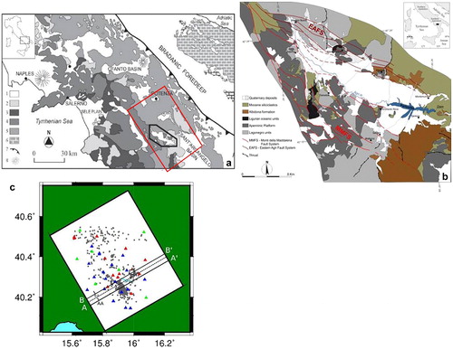
Figure 1. (a) Geological sketch map of the southern Apennines (modified from Giano 2011). Legend: 1 – Plio-Quaternary clastics and volcanics deposits; 2 – Miocene siliciclastic syntectonic deposits; 3 – Cretaceous to Oligocene ophiolite-bearing internal units; 4 – Meso-Cenozoic shallow-water carbonates of the Apennine platform (Appeninic Platform in figure 1b); 5 – Lower-Middle Triassic to Miocene shallow-water and deep-sea successions of Lagonegro units (Lagonegro units in figure 1b); 6 – Meso-Cenozoic shallow water carbonates of the Apulian platform; 7 – Thrust front of the chain; 8 – volcanoes. The red rectangle delimits the tomographic grid represented in figure 1c. (b) Geological sketch map of the Agri basin (modified from Telesca et al. 2015). (c) Investigated area by the tomographic inversion. The rotated box represents the investigated region; grey dots identify all earthquakes used in the tomographic study. The triangles are the stations: red) ENI stations; green) INGV + ISNet stations; blue) INGV 2005–2006 temporary network stations. Also the traces of the sections shown in Figure 13 are reported (solid black lines). The trace of the section reported in Figure 15 is represented by the dashed black line. Along this section, the top of Apulian Platform by Nicolai and Gambini (2007) has been extracted. The white rectangle represents the CM2 injection well. Also the Pertusillo artificial lake is reported.

The genesis of HAV basin is directly linked to the Pleistocene-Holocene, transtensional phase which replaced the Mio-Pliocene compression from which southern Apennines belt originated (Patacca and Scandone 1989). The compressional phase developed by means of two different stages: a Miocenic thin-skinned tectonics and a late-Pliocene early-Pleistocene thick-skinned stage. The former is responsible of the stack of a pile of rootless nappes which constitute the main outcropping units on the western and eastern side of the basin (Dewey et al. 1989; Patacca and Scandone 1989; Valoroso et al. 2011).The Meso-Cenozoic carbonates of Apennine platform and successions of Lagonegro units outcrop along the western side and in the northern side of the HAV, respectively. On the other hand, along the south-eastern side of the basin mainly Miocenic siliciclastic deposits outcrop. The thick-skinned tectonic stage, instead, cut the Inner Apulian Platform (IAP) and the underlying basement with steep reverse faults. deforming the 6–8 km thick Apulian carbonates through large-wavelength anticlines.

The distensive tectonics, on the other hand, was accommodated by two parallel, oppositely dipping, NW striking faults systems. First, the Eastern Agri Fault System (EAFS) developed: it dips to SW and refers to the Early-Middle Pleistocene initial extensional phase (Cello et al. 2003). After that, the Monti della Maddalena Fault System (MMFS) originated: it is a NE dipping normal fault system running about 25–30 km and bordering the HAV to SW. It is a more recent fault system and has not yet created an evident tectonic landscape (Maschio et al. 2005). Although the distensive phase is more recent, the main features that modelled the landscape and the crustal structure of the area still remain the compressive ones (Mazzoli et al. 2000; Menardi Noguera and Rea 2000; Shiner et al. 2004).

Present-day seismicity in the HAV is mainly caused by:

1. continued reservoir induced seismicity associated with the Pertusillo artificial lake (Valoroso et al. 2009; Stabile et al. 2014a);

2. fluid-induced microseismic swarms due to the injection through a single well (Costa Molina 2, CM2 hereafter) of the wastewater produced from the exploitation of the Val d’Agri oil field (Stabile et al. 2014b; Improta et al. 2015).

In addition to this, a natural, very sparse, low-magnitude earthquake activity is detectable ($M_{\mathrm{L}}\le 3.2$). However, this area remains one of the most seismic in Italy since the historical catalogue (CPTI11, Rovida et al. 2011) indicates seven events with Mw ≥4.5 including the 1857 Mw 7.0 Basilicata earthquake. The issue about which of the two extensional fault systems is responsible for the seismogenic potential of the area is still debated. Many authors ascribe it to the EAFS [Figure 1(b)] (Benedetti et al. 1998; Cello and Mazzoli 1999; Borracini et al. 2002; Cello et al. 2003; Barchi et al. 2007). Other researchers attribute the seismogenic potential to MMFS [Figure 1(b)] (Valensise and Pantosti 2001; Maschio et al. 2005; Burrato and Valensise 2008).

On these grounds, many seismological studies were carried out in the last decade starting from analysis of earthquake data recorded by seismic networks deployed in the area. The main aims were to characterize the crustal structure of the area and the different kinds of seismicity involving the HAV. These goals were achieved by means of local earthquake tomographies (Valoroso et al. 2011; Improta et al. 2017), earthquake relocations, focal mechanisms and statistical analyses (Valoroso et al. 2009; Stabile et al. 2014a, 2014b; Improta et al. 2015; Stabile et al. 2015; Telesca et al. 2015; Buttinelli et al. 2016; Improta et al. 2017) and joint Vp/Vs and attenuation studies (Wcisło et al. 2018).

3. Data and methods

In this work, we used seismic data collected in the period January 2002–December 2012 mainly by two seismic networks: a permanent monitoring network operated by ENI Oil Company since 2001 and a temporary network installed in the period May 2005 to June 2006 by INGV. The former consists of 15 triggering mode, Triaxial Lennartz LE-3-D 1 Hz geophones and connected to MARS-88/MC–Lennartz electronic digital data loggers. The latter consists of 27 three-component short-period stations whose data were made available by Improta et al. (2017). In addition to them, very few data recorded by ISNet seismic network stations (Weber et al. 2007; Stabile et al. 2013) and Rete Sismica Nazionale (RSN) instruments, managed by INGV, were also used. The map of the stations is represented in Figure 1(c). The total number of collected earthquakes by the two seismic networks is 2386: 1787 recorded by the ENI network and additional 599 earthquakes recorded only by the INGV temporary network. Preliminary earthquake locations were performed in a mono-dimensional P-wave velocity model of the area (Valoroso et al. 2009) through the probabilistic, absolute earthquake location algorithm NonLinLoc (Lomax et al. 2000). Two separate datasets were obtained by applying the following selection criteria on the detected and located earthquakes: azimuthal gap lower than 200°, RMS time residuals lower than 1 s, a minimum number of 4 P-wave and 2 S-wave arrivals for each source, with picking uncertainty lower than 0.5 s, and, finally, maximum hypocentral depth of 15 km. In that way a first dataset (dataset A hereafter) consisting of 984 earthquakes with 7277 P- and 5567 S-phases recorded only by ENI stations was obtained. The integration of selected data recorded by temporary INGV stations provided a second dataset (dataset B) consisting of an overall number of 1580 earthquakes with 27,257 available P- and S-phases (15,004 and 12,253, respectively).

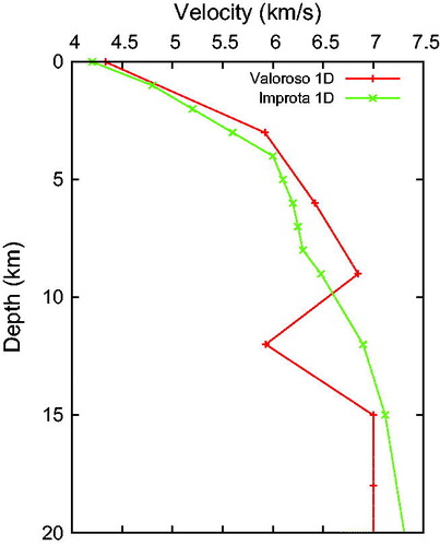
The linearized iterative Simulps‐14q inversion procedure, developed originally by Thurber (1983) and modified by Eberhart‐Phillips and Reyners (1997), was adopted for the tomographic inversion. It uses an iterative damped least-squares method to simultaneously determine 3D Vp and Vp/Vs models and 3D earthquake locations due to hypocentre-velocity structure coupling non-linear problem (Crosson 1976; Menke 1984; Thurber 1992). The crustal volume is described by a three-dimensional grid of nodes. A certain value of Vp and Vp/Vs is assigned to each node, and the seismic velocities in the volume are continuously defined by a trilinear interpolation function from surrounding nodes. The choice of the grid spacing, that is the distance between two adjacent nodes, is a crucial aspect of a tomographic inversion. Actually, it defines the degree to which the parameterization can reproduce structural heterogeneities. On the one hand, a very dense parameterization will allow to reproduce with greater fidelity some structures in the crust (Toomey and Foulger 1989); on the other hand, a too fine grid spacing may produce seismic artefacts and false anomalies. Furthermore, “fine grid spacing yields low resolution estimates, whereas coarse grid spacing yields high resolution estimates” (Husen et al. 2003). In addition to this, to ensure numerical stability to the tomographic inversion also the choice of damping parameters, both for Vp and Vp/Vs inversion, is very important. To determine the best combination of damping parameters for Vp and Vp/Vs models we adopted a recursive procedure (Rawlinson et al. 2006) based on the analysis of trade-off curves between model variance and data variance for single iteration inversions (Eberhart-Phillips 1986). The damping values providing the best compromise between reduction of data variance and increasing of model variance were chosen. Also the maximum Vp and Vp/Vs adjustments for each iteration of the inversion were selected by looking at the curve providing the lowest data variance (Figure S6 in Supplementary Material). Finally, due to the linearized nature of the method, starting solutions, both for earthquake hypocentres and for velocity models, are required. For initial earthquake locations, the results of the preliminary location were used. In order to investigate the dependence of the final solution on the starting velocity model (Kissling et al. 1994), two mono-dimensional Vp models were adopted: Valoroso et al. (2009) 1D velocity model and the one obtained by Improta et al. (2017), both of them adapted for a three-dimensional grid (Figure 2). An homogeneous Vp/Vs value equal to 1.90 was used for the Vp/Vs starting velocity model, as inferred for both datasets from the application of modified Wadati diagram (Chatelain 1978), under the assumption of homogeneous media (Figure S1 in Supplementary Material).

Figure 2. 1D velocity models adopted in the tomographic inversion as starting solutions. Red) 1D velocity model by Valoroso et al. (2009). Green) 1D velocity model by Improta et al. (2017).

3.1. Grid and inversion parameters (Dataset A and Dataset B)

The selected earthquake-station distribution allowed us to investigate a crustal volume of 45 × 60 × 19 km³ for the inversion of dataset A. The slightly different distribution of stations led to enlarge the investigated crustal volume up to 50 × 60 × 19 km³ for inverting dataset B. Since the highest station, in both cases, has altitude of 1542 m a. s. l, the top of the grid was placed 2 km a. s. l. In order to obtain a ray coverage as homogeneous as possible, the tomographic grid was rotated 30° counterclockwise; indeed, the earthquake-station distribution is mainly aligned along a NW-SE direction [Figure 1(c)]. In order to choose the best grid parameterization, the following procedure was followed:

1. Valoroso et al. (2009) 1D Vp model was used as starting velocity model;

2. Three different model parameterizations were implemented, having in common the same vertical grid spacing (2 km above 10 km depth, 3 km below 10 km depth), but different for the horizontal node spacing: (a) 5 × 8 km; (b) 5 × 5 km; (c) 3 × 3 km, in the central part of the tomographic grid;

3. For each of the three parameterizations, the proper combination of damping parameters was chosen following the empirical approach above described: the selected parameters are summarized in Tables 1 and 2, for datasets A and B, respectively;

4. Four iteration inversions were run for each of the three parameterizations; the number of 4 iterations was chosen since it was observed that, independently on the grid spacing, at that step the most of RMS reduction was achieved;

5. Synthetic checkerboard tests (Leveque et al. 1993; Zelt 1998) were performed: the final velocity models were modified by adding positive and negative velocity perturbations of ±0.2 km/s and ±0.095 for Vp and Vp/Vs models, respectively. By using the real source-station configuration, a synthetic arrival-time dataset was retrieved in the checkerboard structure models through a forward travel time computation; after that, synthetic data were inverted by using the same regularization parameters adopted in the four iteration inversions. The same procedure was followed for both datasets.

Table 1. Summary of regularization parameters adopted in the tomographic inversion of dataset A for different model parameterizations.

	Damping Vp (s^2)		Damping Vp/Vs		Max dVp (km/s)		Max dVp/Vs
Node Spacing (km)	Valoroso	Improta	Valoroso	Improta	Valoroso	Improta	Valoroso	Improta
5 × 8 × 2	60	70	60	70	1.0	1.0	0.2	0.15
5 × 5 × 2	70		60		1.2		0.15
3 × 3 × 2	70		50		1.0		0.2

For the vertical spacing, for sake of simplicity, we only referred to the spacing between nodes down to 10 km depth. Max dVp (dVp/Vs) means the maximum Vp (Vp/Vs) adjustment allowed per iteration. For the coarsest grid spacing, also the regularization parameters used in the inversion starting from Improta et al. (2017) P-wave velocity model are provided.

Table 2. Summary of regularization parameters adopted in the tomographic inversion of dataset B for different model parameterizations.

	Damping Vp (s^2)		Damping Vp/Vs		Max dVp (km/s)		Max dVp/Vs
Node spacing (km)	Valoroso	Improta	Valoroso	Improta	Valoroso	Improta	Valoroso	Improta
5 × 8 × 2	70	70	70	80	1.0	1.0	0.2	0.2
5 × 5 × 2	65		70		1.4		0.25
3 × 3 × 2	70		10		1.0		0.25

For the vertical spacing, for sake of simplicity, we only referred to the spacing between nodes down to 10 km depth. Max dVp (dVp/Vs) means the maximum Vp (Vp/Vs) adjustment allowed per iteration. For the coarsest grid spacing, also the regularization parameters used in the inversion starting from Improta et al. (2017) P-wave velocity model are provided.

Figure 3 shows the comparison of the derivative weighted sum (DWS) maps (Toomey and Foulger 1989) obtained for three different parameterizations in the case of inversion of dataset A. It emerges that the coarsest parameterization allowed to retrieve an homogeneous ray coverage in a wider volume with respect to finer parameterizations. Figure 4 [at the end of the section] shows, for the same dataset, the results of the synthetic checkerboard test for P waves: also in this case, the best recovery was achieved with the coarsest node spacing. The parameterization (b) and (c) were not able to recover finer anomalies at the scale of the tested node spacings. Equivalent maps for S-waves (both DWS maps and checkerboard tests) are provided in the supplementary material (Figures S2 and S3 in Supplementary Material). Figure 5 [at the end of the section] shows the comparison of arrival-time residuals at the 4th iteration, both for P- and S-waves, obtained with different parameterizations, from the coarsest to the finest one. It emerges that the increase of number of parameters did not provide a meaningful contribution to the reduction of arrival-time residuals. This observation is expressed by the corrected Akaike information criterion (AIC_c) (Cavanaugh 1997), which is a statistical comparison (Akaike 1974) between models characterized by a different number of used parameters. The computed AIC_c for different node spacings are summarized in Table 3: the minimum AIC_c value, representing the best compromise between reduction of data misfit and model simplicity, was obtained with 5 × 8 km² horizontal parameterization which, therefore, was chosen as the best horizontal node spacing. The same described analyses were performed also for the tomographic inversions of dataset B. The DWS maps, the checkerboard tests and plots of arrival-time residuals are reported in Figures 6–8, respectively. By observing them, and also by looking at the results of statistical analyses summarized in Table 4, we may assert that also for dataset B the best horizontal model parameterization is again 5 × 8 km². Figures concerning DWS maps and checkerboard tests for S-waves are provided in the supplementary material (Figures S4 and S5 in Supplementary Material).

Figure 3. Derivative weighted sum for different model parameterizations relative to dataset A. Each parameterization has a 2-km spacing in the vertical direction up to 10 km depth and 3 km spacing for greater depths. Horizontal plane views are shown for 2 and 4 km depths. These are the model slices characterized by highest values of diagonal elements of resolution matrix. The crosses mark positions of nodes of the tomographic grid. (a) Irregular grid spacing: in the central part of the tomographic grid the node spacing is 5 km and 8 km in the two horizontal directions (x and y), respectively. (b) Regular grid spacing: the horizontal grid spacing is 5 km. (c) Irregular grid spacing: in the central part of the grid, the node spacing is 3 km in both horizontal directions. The coarser parameterization, (a), allows to retrieve a more homogeneous ray coverage in a wider volume with respect to finer parameterizations. For each parameterization, at a single node a much greater DWS value than remaining nodes is observed. It is due to Pertusillo artificial lake seismicity cluster, where most of the earthquakes of our dataset is located.

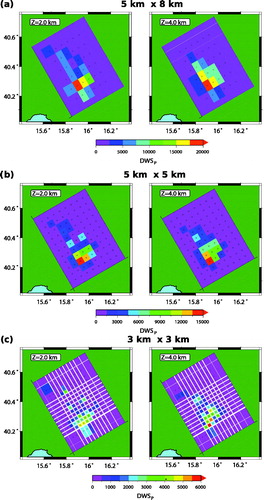
Figure 4. Checkerboard tests relative to dataset A. Left panel of each row represents the actual checkerboard structure, whereas the central and the right panels show the recovered structure after inversion of synthetic travel time data at two different depths (that are the slices of the tomographic grid characterized by highest values of diagonal element of resolution matrix). (a) Irregular grid spacing: in the central part of the tomographic grid, the node spacing is 5 km and 8 km in the two horizontal directions (x and y), respectively. (b) Regular grid spacing: the horizontal grid spacing is 5 km. (c) Irregular grid spacing: in the central part of the grid, the node spacing is 3 km in both horizontal directions. The best recovery of the checkerboard structure is clearly obtained with the coarser parameterization (a).

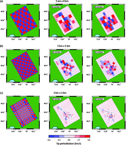
Figure 5. (a) P-waves. Left: Travel time residuals vs epicentral distance for the initial (red dots) and final velocity models obtained with different model parameterizations (blue = 3 × 3 × 2 km³, green = 5 × 5 × 2 km³, purple = 5 × 8 × 2 km³). These plots refer to tomographic inversions of dataset A. Right: corresponding histogram of travel time residuals. The same colour code is used. (b) S-waves. Equivalent plots of Figure (a) are provided. It is clear that, by increasing the number of parameters and tightening the node spacing, the reduction of travel time residuals does not change too much with respect to coarser parameterization.

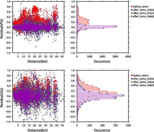
Figure 6. Derivative weighted sum for different model parameterizations relative to dataset B. Each parameterization has a 2-km spacing in the vertical direction up to 10 km depth and 3 km spacing for greater depths. Horizontal plane views are shown for 2 and 4 km depths. These are the model slices characterized by highest values of diagonal elements of resolution matrix. The crosses mark positions of nodes of the tomographic grid. (a) Irregular grid spacing: in the central part of the tomographic grid the node spacing is 5 and 8 km in the two horizontal directions (x and y), respectively. (b) Regular grid spacing: the horizontal grid spacing is 5 km. (c) Irregular grid spacing: in the central part of the grid, the node spacing is 3 km in both horizontal directions. The coarser parameterization, (a), still allows to retrieve an homogeneous ray coverage in a wider volume with respect to finer parameterizations. For each parameterization, at a single node a much greater DWS value than remaining nodes is observed. It is due to Pertusillo artificial lake seismicity cluster, where most of the earthquakes of our dataset is located.

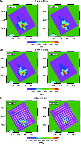
Figure 7. Checkerboard tests relative to dataset B. Left panel of each row represents the actual checkerboard structure, whereas the central and the right panels show the recovered structure after inversion of synthetic travel time data at two different depths (that are the slices of the tomographic grid characterized by highest values of diagonal element of resolution matrix). (a) Irregular grid spacing: in the central part of the tomographic grid, the node spacing is 5 and 8 km in the two horizontal directions (x and y), respectively. (b) Regular grid spacing: the horizontal grid spacing is 5 km. (c) Irregular grid spacing: in the central part of the grid, the node spacing is 3 km in both horizontal directions. The best recovery of the checkerboard structure is clearly obtained with the coarser parameterization. In spite of the increase in the number of data, the small scale anomalies still remain unrecovered.

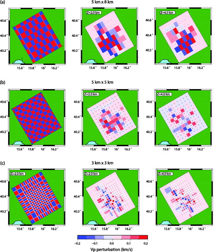
Figure 8. (a) P-waves. Left: Travel time residuals vs. epicentral distance for the initial (red dots) and finals velocity models obtained with different model parameterizations (blue = 3 × 3 × 2 km³, green = 5 × 5 × 2 km³, purple = 5 × 8 × 2 km³). These plots refer to tomographic inversions of dataset B. Right: corresponding histogram of travel time residuals. The same colour code is used. (b) S-waves. Equivalent plots of figure (a) are provided. It is clear that, by increasing the number of parameters and tigthening the node spacing, the reduction of travel time residuals does not change too much with respect to coarser parameterization.

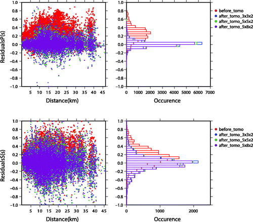
Table 3. Corrected Akaike information criterion (AIC_c) for inversion of dataset A.

Node spacing (km)	Final RMS (s)	No. of parameters	AICc
5 × 8 × 2	0.19	5216	11471
5 × 5 × 2	0.19	6536	26608
3 × 3 × 2	0.19	7836	40189

Table 4. Corrected Akaike Information Criterion (AIC_c) for inversion of dataset B.

Node spacing (km)	Final RMS (s)	No. of parameters	AICc
5 × 8 × 2	0.17	7760	1145
5 × 5 × 2	0.16	9180	6723
3 × 3 × 2	0.16	10,220	11007

In conclusion, the tomographic volume was parameterized with a 5 × 8 × 2 km³ grid spacing down to 10 km depth, and 5 × 8 × 3 km³ at greater depths.

4. Tomographic inversion

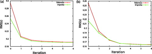
Arrival-time data belonging to both datasets were first inverted by using the 1D P-wave velocity model by Valoroso et al. (2009) as starting solution. The adopted regularization parameters are summarized in Tables 1 and 2. For dataset A, the inversion was stopped at the 5^th iteration, as the model is not significantly modified afterward: it provided a final solution reducing the variance of arrival-time residuals of 57% to a final value of 0.03 s². For dataset B, the inversion, instead, was stopped at the 4th iteration, providing a reduction of variance of arrival-time residuals of 59%, to a final value of 0.03 s². Both datasets were inverted also by using as starting solution the 1D P-wave velocity model by Improta et al. (2017): the adopted regularization parameters are summarized in Tables 1 and 2. We stopped the tomographic inversion of dataset A at the 5th iteration. The variance of arrival-time residuals was reduced of 42% to a final value of 0.03 s². The inversion of dataset B, on the other hand, was stopped at the 6th iteration, providing a reduction of data variance of 43%, to a final value of 0.03 s². The lower reduction of variance of arrival-time residuals achieved by using Improta et al. (2017) 1D P-wave velocity model as starting solution is due to the greater closeness of this initial solution to the real one, as witnessed by the lower initial RMS (Figure 9).

Figure 9. Comparison of RMS vs Iteration curves for tomographic inversions starting from two different initial P-wave velocity models. (a) Inversion of dataset A. (b) Inversion of dataset B.

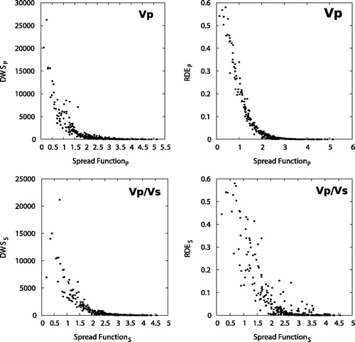
For the representation of the inversion results, it is important to define a resolution threshold level. To this purpose, we introduce here the concept of Spread Function (SF), which is a parameter that is calculated by compressing each row of the resolution matrix into a parameter describing how peaked the resolution is: the lower the SF the more peaked is the resolution (Toomey and Foulger 1989; Michelini and McEvilly 1991). A plot of DWS and Resolution Diagonal Element (RDE) versus the SF value for all nodes, allows defining a maximum SF value for resolved nodes (Dias et al. 2007). In Figure 10 we show these plots, both for Vp and Vp/Vs models, in the case of the inversion of dataset A. The analysis of Figure 10 reveals that for SF > 2 the resolution is very low, whereas well-resolved nodes are characterized by SF < 1.5, both for Vp and Vp/Vs models. Therefore, following Dias et al. (2007), we decided to locate SF threshold value in the middle value between 1.5 and 2.0, that is SF = 1.7. The same analysis was carried out for dataset B inversion: in this case, for the Vp model a SF threshold value equal to 1.5 was chosen, whereas for Vp/Vs model SF = 1.7 is adopted.

Figure 10. Plots of the derivative weight sum (DWS, left) and diagonal element of resolution matrix (RDE, right) versus the spread function (SF) values for the Vp (top) and Vp/Vs (bottom) models.

5. Tomographic results

5.1. Vp and Vp/Vs 3D models

The computed Vp and Vp/Vs models are both represented in map views in Figure 11 [at the end of first paragraph in this section] and Figure 12, respectively. In particular, both images compare final velocity models obtained either inverting the dataset A or inverting the dataset B; furthermore, the comparison between final solution retrieved from the two different initial reference models already introduced are provided. The horizontal planes were chosen to be coincident with the position of the grid nodes in order to reduce interpolation smoothing effects. Each map shows a contour line representing the limits of the resolved area, defined by the chosen threshold SF value. The most resolved area is located at depths between 2 and 4 km and includes both seismicity clusters located NE and SW of the Pertusillo artificial lake.

Figure 11. Map views of the 3D Vp models retrieved after tomographic inversion. For each plot, the small dark grey crosses represent the node position in the tomographic grid. The Pertusillo artificial lake is shown on each plot. The white box identifies the position of wastewater injection well, Costa Molina 2 (CM2). The thin grey line in the z = 0 km panels represents the limits of the quaternary HAV. The grey dots identify the position of located earthquakes: sources far up to 1 km from the slice are projected on the map. The black contour defines the resolved part of the velocity model: the threshold was identified in the way described in the main text. Slices down to 8 km depth are represented since the resolved part of the model for greater depths is negligible. (a) Results of the inversion of dataset A, by using 1D P-wave velocity model by Valoroso et al. (2009) as starting solution. (b) Results of the inversion of dataset A, by using 1D P-wave velocity model by Improta et al. (2017) as starting solution. (c) Results of the inversion of dataset B, by using 1D P-wave velocity model by Valoroso et al. (2009) as starting solution. (d) Results of the inversion of dataset B, by using 1D P-wave velocity model by Improta et al. (2017) as starting solution.

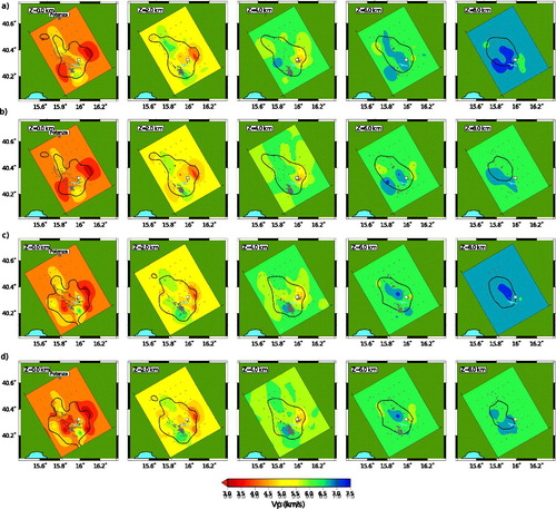
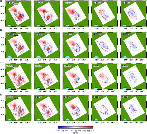
Figure 12. Map views of the 3D Vp/Vs models retrieved after tomographic inversion. For each plot, the small dark grey crosses represent the node position in the tomographic grid. The Pertusillo artificial lake is shown on each plot. The white box identifies the position of wastewater injection well, Costa Molina 2 (CM2). The thin grey line in the z = 0 km panels represents the limits of the quaternary HAV. The grey dots identy the position of located earthquakes: sources far up to 1 km from the slice are projected on the map. The black contour defines the resolved part of the velocity model: the threshold was identified in the way described in the main text. Slices down to 8 km depth are represented since the resolved part of the model for greater depths is negligible. (a) Results of the inversion of dataset A, by using 1D P-wave velocity model by Valoroso et al. (2009) as starting solution. (b) Results of the inversion of dataset A, by using 1D P-wave velocity model by Improta et al. (2017) as starting solution. (c) Results of the inversion of dataset B, by using 1D P-wave velocity model by Valoroso et al. (2009) as starting solution. (d) Results of the inversion of dataset B, by using 1D P-wave velocity model by Improta et al. (2017) as starting solution.

The Vp tomographic images show very similar features, irrespective of the way the final solutions were retrieved. Both low and high Vp anomalies with respect to the mono-dimensional P-wave velocity models are present. In general, an increase with depth of the average P-wave velocities were found, reflecting the main feature of starting velocity models.

At 0 km depth, the retrieved continuous 3D velocity models mainly show two high Vp anomalies (Vp up to 6.0 km/s) located south of the Pertusillo artificial lake and north of the High Agri Valley, respectively. At the eastern limit of the resolved part of this tomographic slice, very low Vp values were retrieved (<3.5 km/s). West of the basin, another similar feature was imaged, even if it is more prominent in the inversion of dataset A than in the inversion of dataset B. In the dataset B images [Figure 11(c,d)], at the western limits of the resolved part of the model, a high Vp anomaly is retrieved. The central part of this slice, corresponding to the Quaternary basin, is characterized by a Vp value very close to the starting one (4.0–4.5 km/s).

The 2 km depth maps show two main features: a low Vp anomaly (<3.5 km/s) ENE of CM2 injection well; an high Vp body (6.0–6.5 km/s) in correspondence of the cluster of seismicity located SW of Pertusillo artificial lake.

At 4 km depth, a low velocity anomaly was found in correspondence of CM2 injection well and of its respective cluster of seismicity.

At 6 km depth and 8 km depth, every Vp models show a high Vp anomaly (6.5–7.5 km/s).

The Vp/Vs models, on the other hand, show a greater complexity. In particular, the inversion of dataset B provided some slightly different features with respect to those retrieved after the inversion of dataset A. In this case, for Vp/Vs models the integration of data contributes to the widening of the resolved part of the model.

At the surface, the area is characterized by very high Vp/Vs values (>2.0), even if results from dataset B, in the resolved part of the model, also show one distinct low Vp/Vs anomaly, south of the Pertusillo artificial lake.

At 2 km depths, all tomographic images show a high Vp/Vs value beneath the Pertusillo artificial lake. Also, the cluster of seismicity located SW of the lake is principally overlapped to high values of Vp/Vs ratio. On the other hand, the CM2 injection well is located in a position of transition between high and low Vp/Vs anomalies. This feature is more evident from the inversion of dataset A than from the inversion of dataset B. Anyway, it is located at the border of the resolved part of the tomographic model. The shallowest earthquakes of the cluster of seismicity NE of the Pertusillo artificial lake are located in correspondence of a high Vp/Vs anomaly.

The 4 km depth maps show low Vp/Vs values beneath the CM2 injection well and its cluster of seismicity; on the other hand, the earthquakes located SW of the Pertusillo artificial lake are correlated with a positive Vp/Vs anomaly.

At 6 km depth, the tomographic images are characterized by Vp/Vs values very close to 1.90, that is the value of the homogeneous Vp/Vs model adopted as starting solution of the tomographic inversion.

At 8 km depth, instead, low Vp/Vs values were mainly retrieved.

We assessed the reliability of tomographic images first by the joint analysis of DWS, RDE, and SF values, as already shown. This helped us to delimit the most resolved parts of the tomographic model. Furthermore, proper checkerboard tests, already introduced in the previous paragraph, were carried out: their complete results are shown in the supplementary material (Figure S7 in Supplementary Material). The comparison of the resolution contour with the results of the checkerboard tests shows that in the resolved part of the model the anomalies of the size of the adopted node spacing are very well recovered. Even if the grid parameterization adopted in the inversion of dataset B was the same of the dataset A, the results of checkerboard test suggest that the former provided more resolved Vp/Vs anomalies than those retrieved from the latter. A further consideration that can be made is the one concerning very high DWS values mainly gathered on a single (or very few) node of the tomographic grid: this is ascribed to the heterogeneous distribution of seismicity in the imaged earth volume. In particular, the highest values of DWS were found in correspondence of the cluster of seismicity SW of the Pertusillo artificial lake, where the most of sources used in the tomographic inversion were located. Furthermore, the comparison between tomographic images, both Vp and Vp/Vs models, retrieved with different starting solutions allows us to assert that the choice of the initial velocity model does not affect the final three dimensional tomographic models.

5.2. Earthquake relocation

Figure 13 shows the earthquake relocation obtained from the inversion of both dataset A and dataset B in two cross sections, cutting seismicity clusters SW and NE of the Pertusillo artificial lake, respectively. The comparison between the starting, absolute hypocentral solutions retrieved in the 1D velocity model of Valoroso et al. (2009) and final ones (red and black dots, respectively) is provided.

Figure 13. Section view of absolute earthquake locations. The traces of the sections are reported in Figure 1c. The two sections were chosen in order to cut the main seismicity clusters present in the area, the one nearby the Pertusillo artificial lake and the one nearby CM2 injection well. The earthquakes far up to 2 km from the section are projected on it. (a) Comparison between initial (red dots) and final (black dots) absolute earthquake locations for dataset A. The inversion was run by using the 1D P-wave velocity model by Valoroso et al. (2009) as starting solution. (b) Comparison between initial (red dots) and final (black dots) absolute earthquake locations for dataset B. The inversion was run by using the 1D P-wave velocity model by Valoroso et al. (2009) as starting solution.

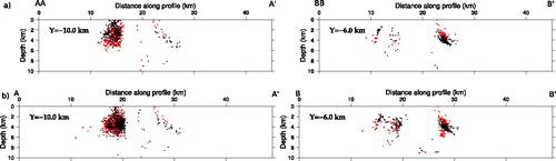
Even if the overall spatial pattern of absolute earthquake locations was not greatly altered, some changes from the starting hypocentral solutions may be observed. In particular, by looking at the northern section (y = −6.0 km) we notice a deepening of the most of the events belonging to the cluster of seismicity induced by wastewater injection at the CM2 well. The most of the earthquakes are confined beneath 3 km depth, even if some hypocentres are also located at shallower depths. An opposite effect is observable on a small number of earthquakes belonging to dataset B [Figure 13(b), section y = −6.0 km]. Their hypocentral positions retrieved in the 3D model are shallower than those relative to 1D earthquake locations. Their final positions are clustered with the other injection induced earthquakes. Thus, an overall north-eastward dipping alignment of located events is defined. This observation is common to results obtained from the inversion of both datasets. The more southern section, on the other hand, shows different results depending on the inverted data. In particular, dataset A provided a very sparse distribution of earthquakes, from very shallow depths up to 6 km depth. The inversion of dataset B, instead, allows to image two distinct clusters, very close to each other, both confined between 2 and 5 km depth which cannot be distinguished in the 1D location.

The earthquake location in a three-dimensional velocity model, furthermore, contributed to reduce average values of earthquake RMS, and horizontal and vertical location errors (Figure 14). In particular, for dataset A, the RMS decreased from 0.120 s to 0.048 s, whereas the dataset B provided an improvement of RMS, which passed from 0.120 s to 0.051 s. The RMS of dataset B is higher than the RMS of dataset A because of the greater number of data. On the other hand, the initial, average, horizontal errors of 0.888 km and 0.801 km for dataset A and dataset B were reduced down to values of 0.461 km and 0.351 km, respectively. Finally, the initial, average, vertical location errors of 1.001 km and 0.903 km for dataset A and dataset B were reduced down to values 0.823 km and 0.661 km.

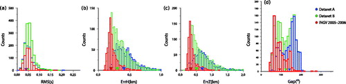
Figure 14. Histograms of the final absolute earthquake location and azimuthal gap of 1D earthquake location. (a): Histogram of arrival-time RMS retrieved from the inversion. Blue) Inversion from dataset A. Green) Inversion from dataset B. Red) Inversion of dataset recorded by the temporary seismic network in the period 2005–2006 and made available by Improta et al. (2017). The earthquakes were relocated in the 3D velocity model by Valoroso et al. (2011). (b) Horizontal errors of the located earthquakes. (c) Vertical errors of the located earthquakes. (d) Azimuthal gap of earthquakes located in the 1D velocity model by Valoroso et al. (2009). The same colour code of the histogram in figure (a) was adopted. For each histogram, the triangles represent the median values of the respective distribution.

6. Discussion

6.1. Velocity model interpretation

The average Vp and Vp/Vs velocities obtained in our work are in agreement with previous tomographic works in the HAV provided by Valoroso et al. (2011) and Improta et al. (2017). Furthermore, the range of imaged velocities is very similar to that retrieved by Amoroso et al. (2014) and Improta et al. (2014) seismic tomographies carried out in Irpinia (Campania-Lucania region); this region, located about 50 km north of the HA, has very similar geological features to those of our investigated area, as already noticed by Improta et al. (2017)

In our Vp models, at 0 km depth, the HAV is characterized by almost homogeneous P-wave velocity values (Vp ∼ 4.3 km/s) with a very high Vp/Vs; furthermore, the shallow high and low Vp anomalies retrieved by the tomographic inversion border the geographical limits of the basin, making clear the distinction between different geological units. The superficial high Vp anomaly south of the basin, located at the border of the resolved part of the tomographic image, partially overlaps the Cretaceous to Oligocene ophiolites outcropping in the Mt. Alpi tectonic window and depicted in the geological map of Figure 1(a). On the other hand, the northern high Vp anomaly is overlapped to outcropping rigid Meso-Cenozoic rocks of Lagonegro basin. The eastern low Vp anomaly, instead, is found in correspondence of Miocenic siliciclastic deposits filling satellite basins, as already found by Valoroso et al. (2011) and Improta et al. (2017). The western high Vp anomaly retrieved from the inversion of dataset B, irrespective of the starting velocity model, is partially overlapped to outcropping units of Apennine platform and Lagonegro units.

The main tomographic features retrieved at 2 and 4 km depths concern those overlapped to clusters of seismicity located SW and NE of the Pertusillo artificial lake. The former is superimposed to an area of high Vp and high Vp/Vs ratio in agreement with results of both Valoroso et al. (2011) and Improta et al. (2017): the imaged high Vp/Vs may be due to the presence of fluids. This may further confirm that this cluster of seismicity is mainly due to a reservoir induced seismic activity. The latter, on the other hand, coincides with low Vp values and from low to average Vp/Vs anomalies. These features are also clearly visible in the section view provided by Figure 15. In particular, at 4 km depth, low Vp/Vs values in the close vicinity of projection at depth of the CM2 well and of the located hypocentres were found. These results are in disagreement with the two previous tomographic studies by Valoroso et al. (2011) and Improta et al. (2017). Indeed, the possible high Vp/Vs values in correspondence of the cluster of seismicity close to the CM2 well imply two consequent conclusions:

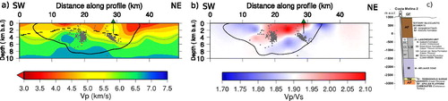
Figure 15. Comparison of tomographic model with subsurface data. (a) Vp section along a profile represented by the dashed black line in Figure 1(c). The green triangle represents the projection of the CM2 well, 3 km far from the traced section, on this profile. The solid black contour line defines the limits of the resolved part of the model. The dashed black line represents the top of Apulian Platform as inferred by Nicolai and Gambini (2007). The top of Apulian Platform was extracted from the intersection of the profile represented by the dashed line in Figure 1(c) and the isolines of map provided by Nicolai and Gambini (2007). The solid grey line represents the 5.8 km/s isovelocity line of the tomographic model. The grey dots represent the located hypocentres in the 3D velocity model. Earthquakes far up to 2 km from the section are projected on it. (b) Vp/Vs section. (c) Stratigraphic log at the CM2 well (from Balasco et al. 2015).

1. Presence of fractured, high pore pressure formations (Nur 1972; Tselentis et al. 2011; Improta et al. 2017).

2. The seismicity is mainly controlled by pressure of fluids (Improta et al. 2017).

Also, Wcisło et al. (2018), in their analyses on seismic data of injection induced cluster collected by stations very close to the CM2 injection well, retrieved high Vp/Vs values. Concerning this, our images are in partial agreement with their study: indeed, the seismic rays, travelling from the cluster of fluid-induced events to stations close to the CM2 well [Figure 15(b)] have ray-paths partially in very high Vp/Vs materials and partially in low Vp/Vs layers. Since high Vp/Vs values retrieved by Wcisło et al. (2018) mainly describe an average representation of the whole properties of the subsurface materials, we think that images retrieved by this study may partially explain their results.

On the other hand, we ascribe the differences between our results and previous tomographic studies to a different degree of detail of the velocity maps. Actually, Valoroso et al. (2011) parameterized the tomographic grid with an homogeneous spacing 3 km ×3 km ×3 km; Improta et al. (2017) obtained very high resolution Vp and Vp/Vs models, with a node spacing of 2 km ×2 km ×1 km. Furthermore, Improta et al. (2017) adopted data acquired in a longer period by a more dense configuration of stations. Thus, a possible interpretation is that the coarser parameterization adopted in this study, with the purpose of providing a spatial resolution as homogeneous as possible in the whole investigated volume, may hinder the imaging of high Vp/Vs anomalies. These features are very useful for detection of fluids in an area characterized by wastewater disposal by a single injection well.

The reliability of the tomographic model retrieved in this study has been further assessed by comparing some main features of our images with available information from subsurface exploration data. The top of Apulian Platform provided by Nicolai and Gambini (2007) has been extracted along the profile represented by the dashed black line of Figure 1(c). Along this profile, the Vp and Vp/Vs sections have been represented in Figure 15. Concerning the Vp section, the 5.8 km/s contour line has been plotted [solid grey line in Figure 15(a)]: indeed, following Shiner et al. (2004), Valoroso et al. (2011) and Improta et al. (2017), it represents the lower limit of the range of velocity values describing the carbonates of the Apulian Platform. We clearly see in the distance interval between 10 km and 20 km a similarity between the trend of the top of the Apulian Platform as inferred by Nicolai and Gambini (2007) and the isovelocity line. In particular, the geometry of the top of the Apulian Platform and of the contour line follows an antiform structure as the ones found by Dell’Aversana (2003), Valoroso et al. (2011), Balasco et al. (2015) and Improta et al. (2017) in their investigations of the area. Furthermore, the depth of 5.8 km/s isovelocity line in this distance interval is very close to the one of the Apulian Platform (the distance between the two curves is lower than 1 km). Since the travel time, Local Earthquake Tomography, due to the mathematical formulation and to the node representation of the tomographic grid, provides a continuous, smooth, velocity model, we think that a so small distance between the two curves is an element of a good reliability of the velocity model in this part of the tomographic grid.

Figure 15 allows also to image low Vp values in correspondence of the injection induced cluster of seismicity close to CM2 well (green triangle in Figure 15). These anomalous low Vp values in the upper part of the Apulian Platform were also found by Improta et al. (2017) along a section profile very close to the one chosen in this study. They interpreted this feature as the effect of a highly fractured area. We also compared the Vp tomographic model with stratigraphic log of the CM2 well (which is about 3 km far from the profile) whose stratigraphy is reported in Figure 15(c). Of course, the parameterization adopted in this study allowed us to retrieve the average velocity model of the area without a detailed discrimination of the seismic velocities of each unit identified in the well log.

6.2. Effects of Local Earthquake Tomography and dataset on absolute earthquake locations

The improvement of absolute earthquake locations retrieved in the tomographic model provided by the inversion of two different datasets is justified by: (a) decrease of the final RMS arrival-time residuals; (b) decrease of the final horizontal and vertical hypocentral errors; (c) clustering of located seismic events (Font et al. 2004).

The updated hypocentral positions allowed us to better delineate the alignment along a NE dipping fault plane of earthquakes belonging to northern cluster of fluid-injection induced seismicity close to the CM2 well. We may notice that the results provided by inversion of dataset A and B are very similar (black dots of right panels in Figure 13). Furthermore, the most of absolute locations of earthquakes obtained in the 3D model are shallower than those retrieved by using the 1D velocity model of Valoroso et al. (2009). Nevertheless, the y = –6.0 km section in Figure 13(b), which is relative to events belonging to dataset B events, allows to highlight a mislocated deep cluster of 44 injection induced earthquakes with hypocentral depth of about 6 km obtained by using the 1D velocity model [Figure 13(b), red dots]. This deep cluster was correctly located at shallower depths when the 3D velocity model was used [Figure 13(b), black dots]. In particular, these mislocated earthquakes were recorded only by the temporary INGV network, whose stations were mainly distributed around the southern cluster of reservoir induced seismicity [as depicted in Figure 1(c)], and were not present in dataset A [see Figure 13(a), right panel]. The less number of available stations for such mislocated deeper induced events is reflected in an azimuthal gap (average value of about 141°) higher than the average gap (about 91°) of whole catalogue of earthquakes recorded in the period 2005–2006 [Figure 14(d)]. Therefore, the 3D velocity model greatly contributes to the better location of events characterized by a poor azimuthal coverage with respect to locations in the 1D model. We already underlined the clustering effect produced by inversion of dataset B on the hypocentral locations of earthquakes located southwest of the Pertusillo artificial lake (Figure 13). This result was not obtained neither when locating earthquakes of both dataset in a 1D velocity model nor when locating sources of dataset A in a three dimensional velocity model. An explanation of this result may be attributed to different geometry of the ENI seismic network with respect to the INGV one. Dataset A only refers to data collected by ENI stations [Figure 1(c)], which, at the expense of a low azimuthal gap, are sparsely distributed in the whole investigated area in order to record earthquakes belonging to both clusters of seismicity. This statement is clearly confirmed by the respective histogram of azimuthal gaps of earthquakes located in the 1D velocity model of Valoroso et al. (2009) and represented in Figure 14(d) (blue histogram).On the other hand, the dataset B is obtained by integrating the dataset A with the arrival-time recorded by stations of the dense temporary network managed by INGV. The most of activity recorded by these stations occurred (about 90% of the total number of events) southwest of the Pertusillo artificial lake. Therefore, a very good azimuthal coverage and a consequent decrease of the azimuthal gap for the most of earthquakes in the period May 2005–June 2006 was provided. Also in this case, the histogram depicted in Figure 14(d) clearly confirms this assertion. This was reflected also on the respective horizontal and vertical errors of absolute earthquake locations represented by the red histogram of Figure 14(b,c): the average horizontal error is lower than those provided by both dataset A and dataset B. This observation agrees with Bondar et al. (2004) study which confirms the importance of a proper network geometry for obtaining high accuracy in epicentre location. Therefore, in our case, we show that the integration of data relative to earthquakes with a very good azimuthal coverage improves the quality of absolute earthquake location in terms of both earthquake clustering and reduction of hypocentral errors.

7. Conclusions

The tomographic inversion of arrival-time data acquired mainly by two seismic networks in the period January 2002 to December 2012 in HAV area allowed us:

1. to retrieve three dimensional Vp and Vp/Vs tomographic images of HAV;

2. to improve the accuracy of absolute earthquake locations with respect to those obtained in a 1D velocity model.

First, we demonstrated that, even if the number of data increased, the inversion of dataset B was not able to image the elastic anomalies at a greater spatial detail with respect to dataset A. Indeed, the grid spacing providing the best compromise between simplicity of the model and reduction of travel-time residuals is 5 km ×8 km ×2 km above 10 km depth and 5 km ×8 km ×3 km at greater depths, independently of the inverted dataset. Anyway, the Vp/Vs anomalies retrieved from the inversion of dataset B are more resolved than those provided by dataset A, as suggested by results of synthetic checkerboard tests.

The reliability of retrieved tomographic images is mainly confirmed by their similarity with those obtained by previous tomographic works in the area. We also compared our velocity model with subsurface exploration data available in literature. Small differences between our tomography and previous ones were found in the 2–4 km depth range, where we were not able to retrieve high Vp/Vs anomaly in correspondence of wastewater injection at the CM2 well (as, instead, imaged by Improta et al. 2017). We think that two ways may be followed in order to better detail this specific area of the HAV: (1) a greater number of data has to be used providing an improvement of the ray coverage; (2) a tomographic multiscale procedure may be adopted (Chiao and Kuo 2001). The former would be possible also on the basis of the collection of data recorded by an experimental temporary seismic network recently installed around the two clusters of induced events in the HAV within the research project INSIEME (Stabile et al. 2018). The latter will be based on a restriction of tomographic grid mainly around the two clusters of seismicity. A further tomographic study should be carried out. The velocity model described in this work will be used as a starting solution; it will be interpolated in a grid characterized by a finer parameterization. Actually, in that way, we will exploit the higher ray coverage around the two clusters of seismicity in order to retrieve a greater detail of the velocity models in that area. Furthermore, the grid spacing in the regions external to the new tomographic grid will remain unchanged: in that way, we will avoid the introduction of artefacts and false anomalies in areas where the resolution due to low ray coverage is very poor.

This study also demonstrated that the improvement of absolute earthquake location accuracy is related to both the network geometry and the availability of a three dimensional velocity model. We compared the clustering of located earthquakes and the horizontal and vertical errors obtained after the inversion of two different arrival-time datasets. These are related to a slightly different station coverage around the recorded earthquakes. We demonstrated that, in the case of the HAV, a very dense seismic network greatly contributes to the improvement of absolute earthquake locations, both in terms of clustering and in terms of hypocentral errors. Furthermore, we observed that the 3D velocity model allows a more reliable estimation of absolute earthquake location with respect to that obtained by using the 1D velocity model. This improvement is particularly evident when the azimuthal coverage of earthquakes is poor.

Acknowledgment

We acknowledge Salvatore Ivo Giano for allowing us to use in this work the figure of the geological setting of the High Agri Valley published in Giano (2011).

Disclosure statement

No potential conflict of interest was reported by the authors.

Additional information

Funding

This work has been funded by the INSIEME project in the framework of the SIR-MIUR program (grant no. RBSI14MN31). We acknowledge two anonymous reviewers for their careful revision that greatly contributed to the improvement of our manuscript.

References

- Akaike H. 1974. A new look at the statistical model identification. IEEE Trans Autom Control. 6:716–723.
- Amoroso O, Ascione A, Mazzoli S, Virieux J, Zollo A. 2014. Seismic imaging of a fluid storage in the actively extending Apennine mountain belt, southern Italy. J Geophys Res. 41:3802–3809. doi:10.1002/2014GL060070.
- Balasco M, Giocoli A, Piscitelli S, Romano G, Siniscalchi A, Stabile TA, Tripaldi S. 2015. Magnetotelluric investigation in the High Agri Valley (southern Apennine, Italy). Nat Haz Earth Syst Sci. 15:843–852. doi:10.5194/nhess-15-843-2015.
- Barchi M, Amato A, Cippitelli G, Merlini S, Montone P. 2007. Extensional tectonics and seismicity in the axial zone of the Southern Apennines. edited by A. Mazzotti, E. Patacca and P. Scandone, Boll. Soc. Geol. Ital., 7:47–56.
- Benedetti L, Tapponier P, King GCP, Piccardi L. 1998. Surface rupture due to the 1857 Southern Italian Earthquake. Terra Nova. 10(4):206–210.
- Bondar I, Myers SC, Engdahl ER, Bergman EA. 2004. Epicentre accuracy based on seismic network criteria. Geophys J Int. 156:483–496.
- Borracini F, De Donatis M, Di Bucci D, Mazzoli S. 2002. 3D model of the active extensional fault system of the high Agri River valley, Southern Apennines, Italy. J. Virtual Expl. 6:1–6.
- Burrato P, Valensise G. 2008. Rise and fall of a hypothesized seismic gap: source complexity in the 16 December 1857, southern Italy earthquake, Mw 7.0. Bull Seism Soc Am. 98(1):139–148.
- Buttinelli M, Improta L, Bagh S, Chiarabba C. 2016. Inversion of inherited thrusts by wastewater injection induced seismicity at the Val d’Agri oilfield (Italy). Sci Rep. 6:37165. doi:10.1038/srep37165.
- Cavanaugh JE. 1997. Unifying the derivations for the Akaike and corrected Akaike information criteria. Stat Probab Lett. 33(2):201–208.
- Cello G, Mazzoli S. 1999. Apennine tectonics in southern Italy: a review. J Geodyn. 27:191–211.
- Cello G, Tondi E, Micarelli L, Mattioni L. 2003. Active tectonics and earthquake sources in the epicentral area of the 1857 Basilicata earthquake (Southern Italy). J Geodyn. 36:37–50.
- Chatelain JL. 1978. Etude fine de la sismicité en zone de collision continentale aumoyen d’un réseau de stations portables: La région Hindu-Kush Pamir. [Detailed study of seismicity in an area of continental collision by using a network of portable seismic stations: Hindu-Kush Pamir region]. [PhD dissertation]. Université scientifique et médicale de Grenoble. 219 pp. French.
- Chen H, Chiu J-M, Pujol J, Kim K, Chen K-C, Huang B-S, Yeh Y-H, Chiu S-C. 2006. A simple algorithm for Local Earthquake location using 3-D Vp and Vs models: test examples in the Central United States and in Central Eastern Taiwan. Bull Seism Soc Am. 96(1):288–305. doi:10.1785/0120040102.
- Chiao L-Y, Kuo B-Y. 2001. Multiscale seismic tomography. Geophys. J. Int. 145:517–527.
- Crosson RS. 1976. Crustal structure modeling of earthquake data. 1. Simultaneous least-squares estimation of hypocenter and velocity parameters. J. Geophys. Res. 81(17):3036–3046.
- De Landro G, Amoroso O, Stabile TA, Matrullo E, Lomax A, Zollo A. 2015. High-precision differential earthquake location in 3-D models: evidence for a rheological barrier controlling the microseismicity at the Irpinia fault zone in southern Apennines. Geophys. J. Int. 203:1821–1831. doi:10.1093/gji/ggv397.
- Dell’Aversana P. 2003. Integration loop of “global offset” seismic, continuous profiling magnetotelluric and gravity data. First Break. 21:32–41. doi:10.3997/1365-2397.2003019.
- Dewey JF, Helman ML, Turco E, Hutton DWH, Knott SP. 1989. Kinematics of the western Mediterranean. In: Coward MP, Dietrich D, Park RG, editors. Alpine tectonics. London: Geological Society, Special Publications, Vol. 45, p. 265–283.
- Di Niro A, Giano SI, Santangelo N. 1992. Primi dati sull’evoluzione geomorfologica e sedimentaria del bacino dell’Alta Val d’Agri (Basilicata).[First data on geomorphological and sedimentary evolution of High Agri Valley basin (Basilicata)]. Studi Geologici Camerti. Special volume. 1992(1):257–263. Italian.
- Dias NA, Matias L, Lourenço N, Madeira J, Carrilhho F, Gaspar JL. 2007. Crustal seismic velocity structure near Faial and Pico islands (AZORES), from Local Earthquake Tomography. Tectonophysics. 445:301–317.
- Eberhart‐Phillips D, Reyners M. 1997. Continental subduction and three‐dimensional crustal structure: The Northern South Island, New Zeland. J Geophys Res. 102:11843–11861. doi:10.1029/96JB03555.
- Eberhart-Phillips D. 1986. Three dimesnional velocity structure in northen California coast ranges from inversion of local earthquake arrival times. Bull Seismol Soc Am. 76(4):1025–1052.
- Font Y, Kao H, Lallemand S, Liu C, Chiao L. 2004. Hypocentre determination offshore of eastern Taiwan using the Maximum Intersection method. Geophys J Int. 158(2):655–675.
- Giano SI, Maschio L, Alessio M, Ferranti L, Improta S, Schiattarella M. 2000. Radiocarbon dating of active faulting in the Agri high valley, southern Italy. J Geodyn. 29:371–386.
- Giano SI. 2011. Quaternary alluvial fan system of the Agri intermontane basin (southern Italy): tectonic and climate controls. Geol Carpathica. 62(1):65–76.
- Gok E, Chavez-Garcia FJ, Polat O. 2014. Effect of soil condition on predicted ground motion: case study from western Anatolia, Turkey. Phys Earth Planet Int. 229:88–97.
- Gomberg JS, Shedlock KM, Roecke SW. 1990. The effect of S-wave arrival times on the accuracy of 557 hypocenter estimation. Bull Seism Soc Am. 80:1605–1628.
- Got JL, Frèchet J, Klein FW. 1994. Deep fault plane geometry inferred from multiplet relative relocation beneath the south flank of Kilauea. J Geophys Res. 99:15375–15386.
- Husen S, Kissling E, Deichmann N, Wiemer S, Giardini D, Baer M. 2003. Probabilistic earthquake location in complex three-dimensional velocity models: application to Switzerland. J Geophys Res. 108(B2):2077. doi:10.1029/2002JB001778.
- Improta L, De Gori P, Chiarabba C. 2014. New insights into crustal structure, Cenozoic magmatism, CO2 degassing, and seismogenesis in the southern Apennines and Irpinia region from Local Earthquake Tomography. J Geophys Res Solid Earth. 119:8283–8311. doi:10.1002/2013JB010890.
- Improta L, Valoroso L, Piccinini D, Chiarabba C. 2015. A detailed analysis of wastewater-induced seismicity in the Val d’Agri oil field, Italy. Geophys Res Lett. 42(8):2682–2690. https://doi.org/10.1002/2015GL063369
- Improta L, Bagh S, De Gori P, Valoroso L, Pastori M, Piccinini D, Buttinelli M. 2017. Reservoir structure and wastewater-induced seismicity at the Val d’Agri oilfield (Italy) shown by three-dimensional Vp and Vp/Vs Local Earthquake Tomography. J Geophys Res Solid Earth. 122(11):9050–9082. https://doi.org/10.1002/2017JB014725
- Kaven JO, Pollard DD. 2013. Geometry of crustal faults: identification from seismicity and implications for slip and stress transfer models. J Geophys Res Solid Earth. 118:5058–5070. doi:10.1002/jgrb.50356.
- Kissling E, Ellsworth WL, Eberhart-Phillips D, Kradolfer U. 1994. Initial reference models in Local Earthquake Tomography. J Geophys Res. 99(B10):19365–19646.
- Lahr JC. 1989. Hypoellipse/version 2.0: A computer program for determining local earthquake hypocentral parameters, magnitude and first motion pattern. U.S. Geol. Surv. 92 pp.
- Lee WHK, Lahr JC. 1972. Hypo-71: A computer program for determining hypocenter, magnitude and first motion pattern of local earthquakes. U.S. Geol. Surv.
- Leveque JJ, Rivera L, Wittlinger G. 1993. On the use of checker-board test to assess the resolution of tomographic inversions. Geophys J Int. 115:313–318.
- Lomax A, Virieux J, Volant P, Berge C. 2000. Probabilistic earthquake location in 3-D and layered models: Introduction of a Metropolis-Gibbs method and comparison with linear locations. In: Thurber CH, Rabinowitz N, editors. Advances in seismic event location. Amsterdam: Kluwer; p. 101–134.
- Maschio L, Ferranti L, Burrato P. 2005. Active extension in Val d’Agri area, Southern Apennines, Italy: implications for the geometry of the seismogenic belt. Geophys J Int. 162:591–609.
- Matrullo E, De Matteis R, Satriano C, Amoroso O, Zollo A. 2013. An improved 1-D seismic velocity model for seismological studies in the Campania-Lucania region (Southern Italy). Geophys J Int. 195:460–473.
- Mazzoli S, Barkham S, Cello G, Gambini R, Mattioni L, Shiner P, Tondi E. 2001. Reconstruction of continental margin architecture deformed by the contraction of the Lagonegro Basin, southern Apennines, Italy. J Geol Soc London. 158:309–319.
- Mazzoli S, Sveva C, De Donatis M, Scrocca D, Butler RWH, Di Bucci D, Naso G, Nicolai C, Zucconi V. 2000. Time and space variability of ≪thin-skinned≫ and ≪thick-skinned≫ thrust tectonics in the Apennines (Italy). Rend Fis Acc Lincei. 11(1): 5–39.
- Menardi Noguera A, Rea G. 2000. Deep structure of the Campanian-Lucanian arc (southern Apennine, Italy). Tectonophysics. 324:239–265.
- Menke W. 1984. Geophysical data analysis: Discrete inverse theory. Academic Press. New York. 260 pp.
- Michelini A, McEvilly TA. 1991. Seismological studies at Parkfield. I. Simultaneous inversion for velocity structure and hypocenters using cubic B-splines parameterization. Bull Seismol Soc Am. 81(2):524–552.
- Nicolai C, Gambini R. 2007. Structural architecture of the Adria platform-and-basin system. Boll Soc Geol Ital Spec Issue. 7:21–37.
- Nur A. 1972. Dilatancy, pore fluids, and premonitory variations of Ts/Tp travel times. Bull Seism Soc Am. 62:1217–1222.
- Patacca E, Scandone P. 1989. Post‐Tortonian mountain building in the Apennines: The role of the passive sinking of a relic lithospheric slab. In: Boriani A, et al., editors. The lithosphere in Italy: advances in earth science research. Atti Conv. Lincei. Vol. 80; p. 157–176.
- Pavlis GL. 1986. Appraising earthquake hypocenter location errors: a complete, practical approach for 623 single event locations. Bull Seism Soc Am. 76:1699–1717.
- Rawlinson N, Reading AM, Kennet BLN. 2006. Lithospheric structure of Tasmania from a novel form of teleseismic tomography. J Geophys Res. 111, B02301:1–21. doi:10.1029/2005JB/2005JB003803.
- Rovida A, Camassi R, Gasperini P, Stucchi M (eds.). 2011. CPTI11, la versione 2011 del Catalogo Parametrico dei terremoti italiani [CPTI11, the 2011 version of the parametric catalogue of italian earthquakes]. Milano, Bologna. http://emidius.mi.ingv.it/CPTI
- Shiner P, Beccaccini A, Mazzoli S. 2004. Thin-skinned versus thick-skinned structural models for Apulian carbonate reservoirs: constraints from the Val d’Agri Fields, S Apennines, Italy. Mar Petrol Geol. 21:805–827.
- Stabile TA, Giocoli A, Lapenna V, Perrone A, Piscitelli S, Telesca L. 2014a. Evidences of low-magnitude continued reservoir-induced seismicity associated with the Pertusillo artificial lake (southern Italy). Bull Seism Soc Am. 104(4):1820–1828.
- Stabile TA, Giocoli A, Perrone A, Piscitelli S, Lapenna V. 2014b. Fluid injection induced seismicity reveals a NE dipping fault in the southeastern sector of the High Agri Valley (southern Italy). Geophys Res Lett. 41:5847–5854. doi:10.1002/2014GL060948.
- Stabile TA, Giocoli A, Perrone A, Piscitelli S, Telesca L, Lapenna V. 2015. Relationship between seismicity and water level of the Pertusillo reservoir (southern Italy). Boll Geof Teor Appl. 56(4):505–517.
- Stabile TA, Iannaccone G, Zollo A, Lomax A, Ferulano MF, Vetri MLV, Barzaghi LP. 2013. A comprehensive approach for evaluating network performance in surface and borehole seismic monitoring. Geophys J Int. 192(2):793–806.
- Stabile TA, Satriano C, Romanelli M, Gueguen E, Serlenga V, Bellanova J, Gallipoli MR, Priolo E, Ripepi E, Saurel JM. 2018. Induced Seismicity in the High Agri Valley (Southern Italy): First Observations from the INSIEME Seismic Network. In SSA Annual Meeting. 14–17 May, Miami.
- Telesca L, Giocoli A, Lapenna V, Stabile TA. 2015. Robust identification of periodic behavior in the time dynamics of short seismic series: the case of seismicity induced by Pertusillo Lake, southern Italy. Stoc Environm Res Risk Asses. 29(5):1437–1446.
- Theunissen T, Chevrot S, Sylvander M, Monteiller V, Calvet M, Villaseñor A, Benhamed S, Pauchet H, Grimaud F. 2018. Absolute earthquake locations using 3-D versus 1-D velocity models below a local seismic network: example from the Pyrenees. Geophys J Int. 212:1806–1828.
- Theunissen T, Lallemand S, Font Y, Gautier S, Lee CS, Liang WT, Wu F, Berthet T. 2012. Crustal deformation at the southern-most part of the Ryukyu subduction (East Taiwan) as revealed by new marine seismic experiments. Tectonophysics. 578(SI):10–30.
- Thurber CH. 1983. Earthquake location and three‐dimensional crustal structure in the Coyote Lake area, central California. J Geophys Res. 88:8226–8236. doi:10.1029/JB088iB10p08226.
- Thurber CH. 1992. Hypocenter-velocity structure coupling in Local Earthquake Tomography. Phys Earth Planet Int. 75:55–62.
- Toomey DR, Foulger GR. 1989. Tomographic inversion of local earthquake data from Hengill-Grensdalur central volcano complex, Iceland. J Geophys Res. 94(B12):17497–17510.
- Tselentis GA, Martakis N, Paraskevopoulos P, Sokos E, Lois A. 2011. High resolution passive seismic tomography (PST) for 3-D velocity, Poisson’s ratio ν, and P-wave quality QP in the Delvina hydrocarbon field, southern Albania. Geophysics. 76(3):B1–B24.
- Valensise G, Pantosti D, 2001. The investigation of potential earthquake sources in peninsular Italy: a review. J Seism. 5:287–306.
- Valoroso L, Improta L, Chiaraluce L, Di Stefano R, Ferranti L, Govoni A, Chiarabba C. 2009. Active faults and induced seismicity in the Val d’Agri area (southern Apennines, Italy). Geophys J Int. 178:488–502. doi:10.1111/j.1365-246X.2009.04166.x
- Valoroso L, Improta L, De Gori P, Chiarabba C. 2011. Upper crustal structure, seismicity and pore pressure variations in an extensional seismic belt through 3-D and 4-D Vp and Vp/Vs models: the example of the Val d’Agri area (southern Italy). J Geophys Res. 116:B07303. https://doi.org/10.1029/2010JB007661
- Waldhauser F, Ellsworth WL. 2000. A double-difference earthquake location algorithm: method and application to the northern Hayward Fault, California. Bull Seism Soc Am. 90:1353–1368.
- Wcisło M, Stabile TA, Telesca L, Eisner L. 2018. Variations of attenuation and Vp/Vs ratio in the vicinity of wastewater injection: a case study of Costa Molina 2 well (High Agri Valley, Italy). Geophysics. 83 (2):B25–B31. doi:10.1190/GEO2017-0123.1
- Weber E, Convertito V, Iannaccone G, Zollo A, Bobbio A, Cantore L, Corciulo M, Di Crosta M, Elia L, Martino C, et al. 2007. An advanced seismic network in the Southern Apennines (Italy) for seismicity investigations and experimentation with earthquake early warning. Seism Res Lett. 78(6):622–634.
- Zelt CA. 1998. Lateral velocity resolution from three-dimensional seismic refraction data. Geophys J Int. 135:1101–1112.