Evaluating the application of the statistical index method in flood susceptibility mapping and its comparison with frequency ratio and logistic regression methods

Abstract

Statistical methods are the most popular techniques to model and map flood-prone areas. Although a wide range of statistical methods have been used, application of the statistical index (Wi) method has not been examined in flood susceptibility mapping. The aim of this research was to assess the efficiency of the Wi method and compare its outcomes with the results of frequency ratio (FR) and logistic regression (LR) methods. Thirteen factors, namely, altitude, slope, aspect, curvature, geology, soil, landuse/cover (LULC), topographic wetness index (TWI), stream power index (SPI), terrain roughness index (TRI), sediment transport index (STI), and distance from rivers and roads, were utilized. A flood inventory was constructed from data captured from the destructive flood that occurred in Brisbane, Australia, in 2011. Model performances were compared using the area under the curve (AUC), Kappa index and five other statistical evaluation tools. The AUC prediction rates acquired for LR, Wi and FR were 79.45%, 78.18%, and 67.33%, respectively. A more realistic representation of the flood-prone area distribution was produced by the Wi method compared to those of the other two techniques. Our research shows that the Wi method can be used as an efficient approach to perform flood susceptibility analysis.

KEYWORDS:

• Flood
• statistical index
• logistic regression
• frequency ratio
• GIS

1. Introduction

Floods are the most prevalent natural disasters worldwide (Khosravi et al. 2016; Gómez-Palacios et al. 2017). This phenomenon is defined as a heavy rainfall that causes rivers to overflow and temporarily cover the neighbouring regions (Merz et al. 2007). Landuse/cover (LULC) and climate change are the two main causes of increases in flood occurrences (Bronstert 2003; Dang and Kumar 2017; Kjeldsen 2010). Climate change has altered the current precipitation pattern, which creates heavy rainfalls in a very short period, quickly forming floods as the extent of rainfall exceeds the permeability capability of the soil. Evidence-based management is required to minimize both biodiversity loss and impacts on human populations and infrastructure from natural disasters (Cinderby and Forrester 2016). If land use and land management practices have the potential to increase flooding, it follows that these also have the potential to mitigate this risk through reduced runoff generation and altered land management (Juarez-Lucas et al. 2016; Shabani et al. 2014). This will require spatially explicit and catchment-scale flood models to test landscape change and rainfall runoff scenarios to reduce the impacts from flooding natural disasters and maintain healthy socio-ecological systems under changing catchment and climate conditions (Tehrany et al. 2015b). Remote sensing and GIS technologies, together with the latest modelling techniques, can contribute to our ability to predict and manage floods (Forte et al. 2006; Pradhan 2010). The existing uncontrolled negative influences of flooding on river coastal socio-ecological communities can be reduced by appropriate preventative actions (Novelo-Casanova and Rodríguez-Vangort 2016).

Flood-prone area mapping has been implemented using various methods in numerous studies. Some of the most popular methods can be categorized into four main groups of hydrological-based (Liu and De Smedt 2004; Jayakrishnan et al. 2005), quantitative (Pradhan and Youssef 2011; Tehrany et al. 2014b; Rahmati et al. 2016), qualitative (Chen et al. 2011; Stefanidis and Stathis 2013) and machine learning (Liong and Sivapragasam 2002; Tehrany et al. 2015a) techniques. Among different groups of flood models presented in the literature, artificial neural networks (ANNs), frequency ratio (FR), logistic regression (LR), decision trees (DT), and support vector machines (SVMs) are the most popular techniques that have been utilized in flood domain mapping (Tehrany et al. 2015b; Mojaddadi et al. 2017). Although flood susceptibility mapping models are available, the reliability of flood prediction maps still remains a critical issue. Each method has different capabilities and can be affected by different sources of uncertainties (Shrestha and Nestmann 2009). Hence, a full understanding of the strength of each model and its uncertainties help us to make a proper choice for each application.

2. Previous studies

Hydrological methods are simple and are based on a nonlinear concept; therefore, they are less effective to model complex features such as the catchments (Sahoo et al. 2009). Traditional flood models have been gradually improved or replaced by rule-based and automated techniques that are more suitable for hazard analyses (Hostache et al. 2013). Some hydrological models, such as SWAT (Anjum et al. 2016) and WetSpa (Nurmohamed et al. 2012) integrate RS and GIS to enhance the accuracy of spatial analysis. However, more robust and precise methods are required to overcome the disadvantages of the traditional hydrological methods. Qualitative methods, such as an analytic hierarchy process (AHP), assesses the flood susceptibility using a multicriteria analysis framework (Karimi et al. 2018). The AHP method has been used by Dahri and Abida (2017) to map the flood-prone areas on the Kassandra Peninsula in northern Greece. These kind of methods require the knowledge of specialists in that specific field. Hence, they cannot be used as reliable techniques due to the involvement of the expert’s opinion in their analysis (Rahmati et al. 2016).

Machine learning techniques, such as ANN (Maier and Dandy 2000), SVM (Tehrany et al. 2015b), and DT (Sun et al. 2011), are widely used in flood analysis. However, a considerable processing time, the requirement of having high performance computing systems along with specific software, and strict selection criteria for input parameters make machine learning methods less usable for a wide range of users (Ghalkhani et al. 2013; Tehrany et al. 2013). SVM, as one of the robust machine learning techniques, has been used by Tehrany et al. (2015b) and Mojaddadi et al. (2017) to map the flood-susceptible areas in various cases of study. The experience required to select a proper SVM kernel, setting the criteria using trial and error, and the complexity of the process make these methods less usable in flood modelling compared to the statistical techniques. Another example is related to the DT technique that provides the tree structure of conditioning factors with corresponding probability weights (Tehrany et al. 2013). There are different forms of decision trees available, such as Logistic Model Trees (LMT), Reduced Error Pruning Trees (REPT), NaïveBayes Trees (NBT), and Alternating Decision Trees (ADT) (Khosravi et al. 2018), that can be used in the spatial modelling. However, similar to SVM, the variety of DT algorithm choices and the requirement for a statistical expert can be considered some of the disadvantages of this technique.

Poor predictions due to the dataset size and dissimilar value ranges of the validation and training datasets are the weak points of ANN (Bui et al. 2016). Due to the weak points of ANN, a neural fuzzy method has been proposed and utilized in several natural hazard applications (Chang and Tsai 2016; Güçlü and Şen 2016). However, the neural fuzzy method has its own restrictions such as its inability to discover optimal weight variables that considerably effect the prediction performance of the model, a slow training speed and a high sensitivity to noise in hydrological modelling (Hong and White 2009). Some hybrid methods, such as the adaptive-network-based fuzzy inference system (ANFIS) and genetic algorithm-based artificial neural network (ANN-GA), have also been applied in flood studies (Chen et al. 2006; Fathzadeh et al. 2017). However, they entail many parameters that restrict their use and reduce their popularity due to data collection difficulties. Moreover, they have long computation times and extra modelling parameters are needed (Dawson et al. 2006).

Deterministic and statistical are two types of quantitative methods. The requirement of having an extensive dataset makes deterministic methods more useful for mapping small regions (Ayalew and Yamagishi 2005). Statistical methods, on the other hand, can be understood with ease within a reasonable period of time (Liao and Carin 2009). As it has been stated by Chau et al. (2005), it is imperative to utilize a quick, understandable, and accurate method for flood modelling. Statistical methods have no specific requirement regarding the input data, software, computer capacity, etc. They can be either bivariate statistical analysis (BSA) (Chen et al. 2018b), multivariate statistical analysis (MSA) (Ayalew and Yamagishi 2005), or a combination of both. BSA evaluates the impact of each class of every conditioning factor on flood occurrence. In contrast, MSA assesses the influence of each factor on flooding, without considering the impact of each class. FR (Khosravi, et al. 2016; Youssef et al. 2016), Weight of Evidence (WoE) (Tehrany et al. 2014b) and Evidential Belief Functions (EBFs) are a few examples of BSA methods. Both WoE and EBF are based on the Dempster–Shafer theory that was first introduced by Shafer (1976). One of the advantages of Dempster–Shafer-based methods is their capability to handle an incomplete dataset. Moreover, they produce predictive flood mapping zones and the degree of uncertainty of the same zone. However, they have a few disadvantages. To use the model, first, the flood conditioning factors should be transformed into evidential data layers (using specific calculations) that can be integrated (by the Dempster–Shafer rule of combination) to generate a predictive flood susceptibility map. This requires several calculation steps and data transformations. In addition, the output result of the Dempster–Shafer parameters (belief, disbelief, uncertainty (doubt), and plausibility) have to be defined as accurately as possible in order to achieve a reasonable final map (Dempster 2008). While these methods are highly useful in some environmental applications, they are less preferable in flood modelling due to the importance of time for data processing.

FR has been utilized by Lee et al. (2012) to map the flood-prone regions in Korea. They stated that the FR method can be quickly and easily applied to areas with little map data, and at low cost. LR is one of the most popular MSA techniques for a variety of applications such as landslides (Chen et al. 2017), floods (Tehrany et al. 2017), land subsidence (Kim et al. 2006), earthquakes (Umar et al. 2014), mineral mapping (Xiong and Zuo 2018), and ground water mapping (Chen et al. 2018a). Unlike most of the statistical methods, LR does not require any pre-analysis assumptions. Additionally, it accepts all data types such as scale, nominal, and categorical. Both FR (Khosravi et al. 2016; Youssef et al. 2016) and LR (Pradhan 2010) have been used in several flood studies; however, the application of the Statistical Index (Wi) has not been tested in this domain. The Wi method is a BSA technique that has been frequently and successfully used in landslide analysis (Yalcin 2008; Bui et al. 2011); however, its application has not been evaluated in other natural hazard studies such as floods, forest fires, groundwater, and soil erosion susceptibility mapping. Hence, the aim of this paper is to apply and examine the proficiency of Wi in flood-prone area mapping. There is no question that natural hazard studies, such as those on flood phenomena, require time and effort in order to provide a better understanding of the flooding problem, and any improvement, no matter how small, will have a considerable impact on the lives of people and on biodiversity.

3. Study area

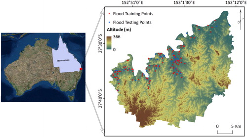
In January 2011, continuous extensive precipitation in the Brisbane Catchment, Australia reduced the infiltration time around the rivers and caused destructive flooding. A lack of proper prevention actions, unorganized need for flood management, deforestation, and urban expansion are the main reasons for an increase in flooding in this region (Bohensky and Leitch 2014). An estimated 200,000 people were affected throughout Queensland during this period, causing damage of an estimated AUD $1 billion (http://www.bom.gov.au/qld/flood/fld_history/brisbane_history.shtml). Most of the area around the Brisbane River flooded, and considerable destruction and loss of life occurred. The Queensland Government undertook a survey regarding the reasons for Brisbane’s 2011 flood and other flood events in the state (QFCI 2012) and the flooding resulted in Australia’s largest class actions to date.

The study areas selected are between 27°23′50.272″S and 27°45′25.078″S latitude and 152°46′17.738″E and 153°11′25.504″E longitude (Figure 1). During the summer, average temperatures range from 21 to 29.8 °C and the city experiences its highest rainfall, which can bring thunderstorms and occasional floods. The average rainfall during this time is 426.6 mm. This area receives approximately 1168 mm of precipitation annually. The minimum amount of precipitation occurs in September (34 mm). February receives the highest amount of rainfall, with an average of 167 mm (http://en.climate-data.org/).

Figure 1. The Brisbane catchment area used in this study, showing the altitude well as training and test point locations.

4. Methodology

The methodology for the current research consists of splitting the flood inventory into training and testing datasets; selecting the appropriate flood-conditioning factors; and undertaking three statistical techniques of FR, LR, and Wi for flood susceptibility and their validations and comparisons.

4.1. Data used

4.1.1. Flood inventory mapping

A flood inventory map is required in order to recognize the correlation among flood conditioning factors and flood incidences (Pradhan et al. 2016; Tehrany and Jones 2017). To produce susceptibility maps, having an accurate and precise record of the past flood events is essential (Merz et al. 2007). Documents regarding the flood event that took place in January 2011 were the main source of the flood inventory used in this research. These data are usually divided into two categories, training, and testing, in order to train the model and validate the outcomes, respectively. Following previous flood modelling studies (Lee et al. 2012; Tehrany et al. 2013; Khosravi et al. 2016), the flood inventory data were randomly grouped into 70% for training and 30% for testing. The locations and distributions of the flood points can be seen in Figure 1.

4.1.2. Flood conditioning factors

The selection of the flood causative factors, known as conditioning factors, is the most influential stage in developing the final flood susceptibility maps and has the highest impact on the precision of the output maps (Kia et al. 2012). Although a lack of a framework or an agreement on how to select the flood conditioning factors still remains, the most relevant and repeatedly used flood conditioning factors by other researchers (Lee et al. 2012; Tehrany et al. 2014a; Rahmati et al. 2016) were used in this study. A flood conditioning factors dataset was constructed using altitude, slope, aspect, curvature, geology, soil, landuse/cover (LULC), topographic wetness index (TWI), stream power index (SPI), terrain roughness index (TRI), sediment transport index (STI), and distance from rivers and roads (Figure 2). A DEM with a 5-meter spatial resolution produced from Light Detection and Ranging (LiDAR) data was used to derive other related topographical and hydrological parameters. ArcGIS (10.2) and SAGA GIS (2.2) software were used to produce the aforementioned conditioning factors. All factors were created in raster format with a 5 m × 5 m pixel size. LR supports all kinds of data types (categorical, scale, nominal, etc.); however, all input factors should be categorized for FR and Wi analysis. The reason for this categorization is that BSA methods, such as FR and Wi, evaluate the impact of each class of every conditioning factor on flood occurrence. Hence, a popular quantile classification method was used to classify scaled factors (altitude, slope, TWI, SPI, TRI, STI, and distance from roads and rivers) into 10 equal classes (Ayalew et al. 2004; Shabani et al. 2018; Tehrany, Shabani, et al. 2017; Tehrany et al. 2017).

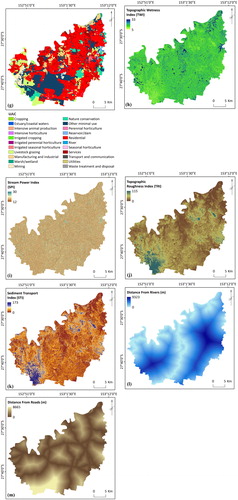
Figure 2. Flood conditioning factors; (a) altitude, (b) slope, (c) aspect, (d) curvature, (e) geology, (f) soil, (g) LULC, (h) TWI, (i) SPI, (j) TRI, (k) STI, (l) distance from rivers and (m) distance from roads.

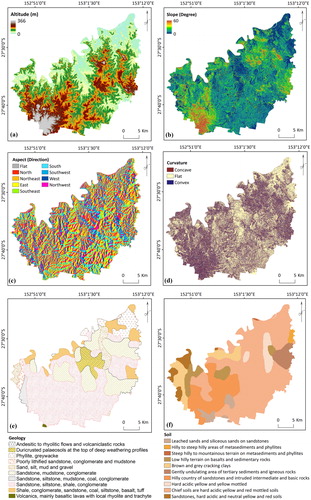
Topographical factors of slope, aspect, and curvature were derived from the DEM. Altitude and slope are two factors that have a considerable impact on flood creation (Pradhan 2009). Floods are generated in the low-lying and flat regions, and it is not possible to have flooding at the peak of mountains (Tehrany et al. 2013). Steep slopes increase the speed of the surface run-off and reduce the time available for the soil to absorb the water. In the case of the aspect factor, this parameter has an impact on the received rainfall and sunshine amount of the terrain (Jebur et al. 2014). Curvature has three classes, flat, convex, and concave, and is another influential parameter in flood studies (Lee and Pradhan 2006). SAGA GIS software was used to generate SPI, TWI, STI, and TRI from the DEM according to the following equations (Jaafari et al. 2014; Jebur et al. 2014):(1) $$\text{TWI}=\ln \left(A_s/\text{tan}\beta \right)\mathrm{ }$$(1) (2) $$\text{SPI}=A_s\text{tan}\beta \mathrm{ }$$(2) (3) $$\text{STI}={\left(\frac{A_S}{22.13}\right)}^{0.6}{\left(\frac{\text{sin}\beta }{0.0896}\right)}^{1.3}\mathrm{ }$$(3) where $A_s$ is the area of the catchment (m²) and β (radians) is the slope gradient. TWI is used to measure topographic control of hydrological procedures (Chen and Yu 2011) and greater TWI values are usually found in flooded areas. SPI represents the erosion power of the stream in the catchment (De Risi 2013). STI defines the movements of the sediments due to the water movement. TRI is one of the morphological factors associated with flooding (Werner et al. 2005). This parameter can be calculated using the following equation:(4) $$\text{TRI}=\sqrt{\text{Abs}\left({\text{max}}^2-{\text{min}}^2\right)}$$(4) where max and min are the largest and smallest values of the cells in the 3 × 3 rectangular neighbourhoods of altitude, respectively. Soil (1:250,000 scale) and geology (1:100,000 scale) data were obtained from the CSIRO and Australian government websites. The study area is covered by different types of soil formations, such as clay and sandstone. Geology is another important flood conditioning factor because it has a considerable impact on the variation in hydrology and sediment production in the catchment (Khosravi et al. 2016). Terrain infiltration, runoff speed, and extent are highly affected by the LULC factor (Kassa 2014). A detailed LULC map was received from the Queensland Land Use Mapping Program (QLUMP) and was produced by the Queensland Government. This map was created by classifying SPOT5 imagery, high spatial resolution orthophotography and scanned aerial photos and using local expert knowledge.

4.2. Flood susceptibility map produced by frequency ratio (FR)

FR is one of the most cited BSA methods in natural hazard studies, such as flood mapping (Jothibasu and Anbazhagan 2016), landslide mapping (Li et al. 2016), ground water mapping (Manap et al. 2014), mineral potential mapping (Yusoff et al. 2015), and soil erosion mapping (Khosrokhani and Pradhan 2014). Its popularity is related to its simple and rapid calculation process (Lee et al. 2012). Equation (5)(5) $$FR=\frac{\left(\frac{N_{pix}\left({SX}_i\right)}{{\sum }_{i=1}^m{SX}_i}\right)}{\begin{array}{c}\left(\frac{N_{pix}\left(X_j\right)}{{\sum }_{j=1}^n{N_{pix}(X}_j)}\right)\end{array}}\mathrm{ }$$(5) shows the calculation of FR for a single conditioning factor, and the flood probability index can be measured by summing the FR of all of the factors (Equation (6)(6) $$FPI=\sum _{j=1}^{n}FR\mathrm{ }\mathrm{ }$$(6) ).(5) $$FR=\frac{\left(\frac{N_{pix}\left({SX}_i\right)}{{\sum }_{i=1}^m{SX}_i}\right)}{\begin{array}{c}\left(\frac{N_{pix}\left(X_j\right)}{{\sum }_{j=1}^n{N_{pix}(X}_j)}\right)\end{array}}\mathrm{ }$$(5) (6) $$FPI=\sum _{j=1}^{n}FR\mathrm{ }\mathrm{ }$$(6) where the number of flooded pixels in class $i$ of the factor $X$ is represented by $N_{pix}\left({SX}_i\right)$; the total number of pixels within factor $X_j$ is represented by $N_{pix}\left(X_j\right)$; $m$ is the number of classes in factor $X_i$; and $n$ is the number of factors in the study area (Regmi et al. 2014).

Microsoft Excel was used to calculate FR for each flood conditioning factor and each factor was reclassified using the derived FR values in ArcGIS 10.2 using a spatial analyst tool. The reclassified factors were added using the raster calculator to produce the flood probability index.

4.3. Flood susceptibility map produced by statistical index (Wi)

Among all the BSA methods, Wi is one of the least used methods in natural hazards modelling and has not been tested in flood susceptibility mapping. The procedure for this method is fast and reasonably simple, which makes it suitable for natural hazard modelling (Aghdam et al. 2016). Wi weights can be described as the natural logarithm of the flood existence in each class of a conditioning factor divided by the total flood density in the study area (Bourenane et al. 2015). The following equation is used to calculate Wi weights for each factor (Chen et al. 2016):(7) $$W_{ij}=\mathrm{I}\mathrm{n}\left(\frac{D_{ij}}{D}\right)=\mathrm{I}\mathrm{n}\left[\left(\frac{N_{ij}}{S_{ij}}/\frac{N}{S}\right)\right]\mathrm{ }$$(7) where the weight received for class $i$ of the conditioning factor $j$ is given by $W_{ij}$; the flood density in class $i$ of the conditioning factor $j$is given by $D_{ij}$; the total flood density within the study area is given by $D$; the number of pixels with flooding in class $i$ of the conditioning factor $j$ is given by $N_{ij}$; the total number of pixels in class $i$ of the conditioning factor $j$is given by $S_{ij}$;$N$ and $S$ are the total number of floods and total number of pixels in the whole study area, respectively.

After deriving the Wi weights for each flood conditioning factor, each factor was reclassified using the derived Wi values in ArcGIS 10.2 using the Spatial Analyst tool. The reclassified factors were added using the raster calculator to produce the flood probability index.

4.4. Flood susceptibility map produced by logistic regression (LR)

LR is an MSA technique that has been frequently used in a wide range of natural hazards analysis (Kang and Zhang 2016; Nandi et al. 2016; Zhang et al. 2016). Defining the specific assumptions are necessary for most of the statistical methods; however, LR does not require any pre-analysis assumptions (Ayalew and Yamagishi 2005). Moreover, all types of conditioning factors (continuous, nominal, categorical, etc.) are supported by LR analysis (Lee 2005). LR evaluates a dependent variable of the specific event (flood) and recognizes the correlation between that event and more than one independent variable (conditioning factor) that may influence the probability of the event. Through LR binary analysis, a regression association among the flood inventory and flood conditioning factors will be undertaken (Mathew et al. 2009). Meaning that, the flood inventory is a binary factor representing the existence and non-existence of the flooding. The flood probability index, which is represented on a S-shaped curve in the range of [0, 1], is the output of this technique. Using the resultant weights (logistic coefficients), the flood probability index (p) was measured as follows (Bai et al. 2012):(8) $$P=\frac{1}{(1+e^{-z}),}$$(8)

$\text{where }Z$ is a linear combination, thus LR involves fitting an equation of the following form to the data:(9) $$z=b_0+b_1{x}_1+b_2{x}_2+b_3{x}_3+b_n{x}_n,$$(9) where the intercept of the method is represented by the constant $b_0$, $b_n\mathrm{ }(n=0,\mathrm{ }1,\mathrm{ }2,\dots ,n)$ represents the LR weights, and $x_n\mathrm{ }(n=0,\mathrm{ }1,\mathrm{ }2,\mathrm{ }\dots ,\mathrm{ }n)$ shows the flood conditioning factors, including slope, aspect, and distance from roads. In the current research, all conditioning factors and the flood inventory map were transformed from raster to ASCII format and transferred to SPSS to perform LR analyses.

4.5. Accuracy assessment

Accuracy assessment is an essential step in every modelling (Bui et al. 2011). In this study, the area under the curve (AUC) method was used to evaluate the efficiency and reliability of the derived three flood probability maps from the FR, Wi, and LR methods. AUC is widely used in natural hazard studies due to its comprehensive, reasonable, and visually understandable method of validation (Yilmaz 2009; Nefeslioglu et al. 2010). It begins with arranging the flood probability index in descending order. Then, the arranged flood probability index is classified into 100 categories on the y-axis, with cumulative 1% breaks on the x-axis. It continues with overlaying the flood inventory on the flood probability index. The presence of the flood points (training and testing) in each class is evaluated, and prediction and success rates are derived (Pourghasemi et al. 2012). Success and prediction rates are two products of the AUC technique. The flood training and testing datasets were used to produce success and prediction rates, respectively. AUC produces a range from zero to one. The method is 100% successful if the AUC value is equal to 1. Hence, the closer the AUC value is to one, the more accurate the technique.

The statistical evaluation measures of overall accuracy, specificity, sensitivity, positive predictive value (PPV), and negative predictive value (NPV) were applied to measure comparative performance of our models (Tien Bui et al. 2016). Overall accuracy, sensitivity, and specificity measure the proportion of training and testing, flooded, and non-flooded samples, respectively, that are correctly classified. PPV and NPV estimate the probability of training and testing dataset samples correctly classified to the flooded class and non-flooded class, respectively.(10) $$\mathit{\text{Overall}}\mathrm{ }\mathit{\text{accuracy}}=\frac{TP+TN}{TP+TN+FP+FN},$$(10) (11) $$\mathit{\text{Specificity}}=\mathrm{ }\frac{TN}{F\mathrm{P}+TN},\mathrm{ }$$(11) (12) $$\mathit{\text{Sensivity}}=\frac{TP}{TP+FN},\mathrm{ }$$(12) (13) $$PPV=\frac{TP}{FP+TP},\mathrm{ }$$(13) (14) $$NPV=\frac{TN}{FN+TN},\mathrm{ }$$(14) where True Positive (TP) and True Negative (TN) are the number of samples in the training and validation datasets, correctly classified to the flood and non-flood class, respectively. False Positive (FP) and False Negative (FN) are the number of samples in the training and validation datasets that were erroneously classified.

5. Results and discussion

5.1. FR outcomes

FR was measured for each class of every flood conditioning factor by dividing the flood occurrence ratio by the area ratio. The derived FR result for each factor is given in Table 1. A greater FR weight shows a stronger association among that class and flood occurrence, and subsequently represents a higher probability of flood occurrence in that class. For instance, the results showed that the first four classes of altitude received the highest FR values. This confirms the concept that flooding mostly occurs in the low-elevated regions. The class ‘0-0.47°’ in the slope map gained the highest FR value of 269.88 among the various classes of slope. Another example is related to the distance from rivers; the closer the distance to the river, the higher the FR weight. The FR-derived flood susceptibility map (Figure 3(a)) was produced by classifying the flood probability index achieved from FR analysis. The flood probability index was categorized into five susceptible zones of very low, low, moderate, high, and very high using the quantile method. The class ‘very high’ covered 9.92% of the study area. The flood-susceptible area distribution in the flood susceptibility map is 9.94% of the area under ‘high’, and 19.93%, 19.98%, and 40.2% of the study area it occupies is ‘moderate’, ‘low’, and ‘very low’, respectively.

Figure 3. Flood susceptibility maps derived from: (a) FR, (b) Wi and (c) LR.

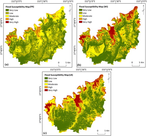
Table 1. The measured FR, Wi and LR for conditioning factor.

Layer	Classes	Cells	Deposit	FR	Wi	LR
Altitude (meters)	0.75–7.87	93,047	30,419	486.36	158.18	0.5907
	7.87–16.49	109,346	31,455	427.96	145.39
	16.49–23.68	104,146	5242	74.88	−28.93
	23.68–30.87	99,440	410	6.13	−279.13
	30.87–38.06	101,823	1	0.01	−883.12
	38.06–45.24	99,110	0	0.00	0.00
	45.24–53.87	107,992	0	0.00	0.00
	53.87–63.93	99,912	0	0.00	0.00
	63.93–79.75	97,263	0	0.00	0.00
	79.75–365.84	92,526	0	0.00	0.00
Slope (Degree)	0–0.47	88,540	16,062	269.88	99.28	1.5919
	0.47–1.17	103,408	11,276	162.23	48.38
	1.175–1.88	108,438	7819	107.27	7.02
	1.88–2.58	117,498	6001	75.98	−27.47
	2.58–3.29	112,639	4748	62.71	−46.66
	3.29–4.23	119,216	4669	58.26	−54.02
	4.23–5.40	102,531	4180	60.65	−50.00
	5.40 - 7.05	86,124	3914	67.61	−39.14
	7.05–10.57	84,932	4446	77.88	−25.00
	10.57–59.92	81,279	4412	80.76	−21.37
Aspect	Flat	8536	2445	426.13	144.96	1.0028
	North	134,772	9242	102.02	2.00
	Northeast	139,425	8883	94.78	−5.36
	East	142,555	8235	85.94	−15.15
	Southeast	114,152	6084	79.29	−23.20
	Southeast	95,915	6343	98.38	−1.63
	Southwest	105,074	7614	107.80	7.51
	West	129,898	9299	106.50	6.30
	Northwest	134,278	9382	103.95	3.87
Curvature	Convex	259,694	13,428	76.92	−26.23	0.9995
	Flat	486,609	41,913	128.14	24.80
	Concave	258,302	12,186	70.19	−35.40
SPI	11.97–12.67	94,145	6557	103.62	3.55	−0.9308
	12.67–12.88	115,416	5381	69.36	−36.58
	12.88–13.45	110,530	8968	120.71	18.82
	13.45–13.80	111,883	6583	87.53	−13.31
	13.80–14.22	103,867	6290	90.09	−10.43
	14.22–14.64	96,776	5776	88.79	−11.89
	14.64–15.20	97,141	6218	95.23	−4.89
	15.20–15.97	93,636	6509	103.42	3.36
	15.97–17.31	93784	7639	121.18	19.21
	17.31–29.88	87,427	7606	129.43	25.80
TWI	5.46–8.41	97,945	5106	77.56	−25.42	1.1242
	8.41–8.95	104,362	5071	72.29	−32.45
	8.95–9.39	103,817	5231	74.96	−28.82
	9.39–9.83	107,728	5814	80.29	−21.95
	9.83–10.26	103,399	5925	85.25	−15.96
	10.26–10.81	114,583	7200	93.48	−6.74
	10.81–11.46	105,687	7084	99.72	−0.28
	11.46–12.34	91,703	6470	104.96	4.84
	12.34–14.19	91,708	6344	102.91	2.87
	14.19–33.29	83,673	13,282	236.15	85.93
TRI	0–1.35	77,331	17,712	340.75	122.60	−0.7039
	1.35–3.15	100,115	21,338	317.08	115.40
	3.15–4.96	122,333	15,289	185.93	62.02
	4.96–6.31	112,598	6483	85.66	−15.48
	6.31–7.66	121,876	3536	43.16	−84.02
	7.66–9.02253	113,222	1607	21.12	−155.52
	9.02–10.82	112,925	893	11.76	−214.01
	10.82–13.53	94,764	488	7.66	−256.90
	13.53–18.94	78,637	167	3.16	−345.48
	18.94–115.03	70,804	14	0.29	−582.88
STI	0–0.67	76,710	14,482	280.86	103.27	−0.9018
	0.67–2.03	113,574	12,710	166.49	50.98
	2.03–3.38	119,717	8548	106.22	6.04
	3.38–4.74	129,815	6382	73.14	−31.28
	4.74–6.09	119,028	4930	61.62	−48.42
	6.09–7.45	94,138	3662	57.87	−54.69
	7.45–9.48	100,101	4081	60.65	−50.00
	9.48–12.86	95,796	4360	67.71	−38.99
	12.86–19.64	81,695	4395	80.04	−22.27
	19.64–172.70	74,031	3977	79.92	−22.41
Distance from Road (Meters)	0–178	101,775	7146	104.46	4.36	1.0003
	178–402	100,680	7418	109.61	9.18
	402–655	100,798	7143	105.43	5.28
	655–936	100,275	7874	116.82	15.55
	936–1259	100,451	9816	145.38	37.42
	1259–1641	100,156	9986	148.33	39.43
	1641–2096	100,123	8099	120.34	18.52
	2096–2667	100,127	6218	92.39	−7.92
	2667–3561	100,200	3780	56.12	−57.76
	3561–8665	100,020	47	0.70	−496.32
Distance from River (Meters)	0–360	100,581	37,312	551.89	170.82	−0.9940
	360–796	100,594	15,141	223.92	80.61
	796–1361	100,438	8848	131.06	27.05
	1361–2047	100,531	3735	55.27	−59.29
	2047–2755	100,432	1791	26.53	−132.69
	2755–3493	100,463	673	9.97	−230.60
	3493–4304	100,500	27	0.40	−552.23
	4304–5237	100,359	0	0.00	0.00
	5237–6362	100,395	0	0.00	0.00
	6362–9323	100,312	0	0.00	0.00
Geology	Sandstone, siltstone, shale, conglomerate	516,130	15,673	23.21	45.18	0
	Phyllite, greywacke	59,248	2088	3.09	52.43	191
	Sand, silt, mud and gravel	45,723	6871	10.18	223.56	0.018
	Sandstone, mudstone, conglomerate	223,469	15,631	23.15	104.06	54.96
	Shale, conglomerate, sandstone, coal, siltstone, basalt, tuff	80,354	10,002	14.81	185.18	0.104
	Andesitic to rhyolitic flows and volcaniclastic rocks	108	0	0.00	0.00	0.991
	Poorly lithified sandstone, conglomerate and mudstone	13,592	4449	6.59	486.96	272.08
	Duricrusted palaeosols at the top of deep weathering profiles	47,992	12,808	18.97	397.04	87.68
	Sandstone, siltstone, mudstone, coal, conglomerate	16,820	5	0.01	0.44	126.5
	Volcanics, mainly basaltic lavas with local rhyolite and trachyte; some plugs	1169	0	0.00	0.00	0
Soil	Leached sands and siliceous sands on sandstones	1059	186	261.30	96.05	0
	Hilly to steep hilly areas of metasediments and phyllites	75,574	23,542	463.43	153.35	0.003
	Steep hilly to mountainous terrain on metasediments and phyllites	36,227	8902	365.57	129.63	0.002
	Low hilly terrain on basalts and sedimentary rocks	29,829	0	0.00	0.00	0.240
	Brown and grey cracking clays	160,242	3845	35.70	−103.01	178.8
	Gently undulating area of tertiary sediments and igneous rocks	557,524	24,349	64.97	−43.12	0.001
	Hilly country of sandstones and intruded intermediate and basic rocks	7913	0	0.00	0.00	0.423
	Hard acidic yellow and yellow mottled	39,227	716	27.15	−130.36	32.287
	Chief soils are hard acidic yellow and red mottled soils	42,068	0	0.00	0.00	0
	Sandstones, hard acidic and neutral yellow and red soils	54,942	5987	162.11	48.31	0
LULC	Reservoir/dam	7140	310	64.59	−43.71	0
	Waste treatment and disposal	2071	294	211.20	74.76	0.001
	Marsh/wetland	2752	0	0.00	0.00	0.013
	Estuary/coastal waters	95	0	0.00	0.00	0.0009
	River	3778	2809	1106.13	240.35	0.0198
	Nature conservation	43,679	145	4.94	−300.81	16.469
	Other minimal use	207,985	8227	58.85	−53.02	0.0310
	Livestock grazing	82,234	13,900	251.47	92.21	12.082
	Cropping	253	59	346.94	124.40	0.0007
	Perennial horticulture	623	0	0.00	0.00	0.0129
	Seasonal horticulture	317	0	0.00	0.00	20.994
	Irrigated cropping	1786	269	224.07	80.68	0.7393
	Irrigated perennial horticulture	3093	0	0.00	0.00	2.8561
	Irrigated seasonal horticulture	3273	0	0.00	0.00	0.8670
	Intensive horticulture	2059	0	0.00	0.00	0
	Intensive animal production	1509	12	11.83	−213.45	0
	Manufacturing and industrial	54,938	7100	192.27	65.37	0
	Residential	453,604	18,177	59.62	−51.72	0
	Services	102,415	15,217	221.05	79.32	0.5151
	Utilities	3284	3	1.36	−429.84	0
	Transport and communication	6181	363	87.37	−13.50	0
	Mining	21,536	642	44.35	−81.31	0

5.2. Wi outcomes

Wi weights for each flood conditioning factor were calculated in Microsoft Excel and ArcGIS 10.2 and are listed in Table 1. The greater the Wi weight for each class of every conditioning factor, the higher the flood occurrence possibility is within that class. Moreover, the negative Wi weights indicate the negative correlation among the class and flood occurrence. For instance, the first three classes of the slope received positive Wi weights; however, the rest of its seven classes gained minus values. This means that by increasing the slope degree, the possibility of flood occurrence decreases.

The Wi technique is based on a statistical correlation of the flood inventory layer with characteristics of the flood conditioning factors classes. Hence, the Wi weights are only measured for flood occurrence classes. If the class does not hold any flood occurrence, it does not have any association with the flood inventory (Bui et al. 2011). Table 1 shows that the highest elevated areas, regions far from rivers, ‘Andesitic’ and ‘Volcanics’ classes of geology; ‘sedimentary rocks’ and ‘hard acidic yellow and red mottled soils’ classes of soil map; ‘marsh’, ‘estuary’, and ‘horticulture’ classes of LULC did not show any correlation with the flood inventory map in this study. Using the weighted sum option in the Spatial Analyst tool of ArcGIS, the final flood probability index was obtained (Figure 3(b)). Similar to the FR analysis, the Wi-derived flood probability index was classified into five susceptible classes using the quantile method. The very high, high, moderate, low, and very low flood-susceptibility zones have area percentages of 7.23%, 12.66%, 20.00%, 19.99%, and 40.12%, respectively.

5.3. LR outcomes

LR analysis was undertaken using SPSS software, and LR coefficients were derived for each flood conditioning factor. Similar to Wi, the negative LR weights indicate that the flood occurrence is negatively associated with the conditioning factor. In this study, SPI, TRI, STI, and distance from rivers received negative weights, and other flood conditioning factors achieved positive weights. The linear combination of the LR constant value and the product of the conditioning factors and their related LR coefficients are given in the following equation:(9) $$\begin{array}{l}Z=\mathrm{ }1134+\left(0.5907\text{\hspace{0.17em}*\hspace{0.17em}Altitude}\right)+\left(1.5919\text{\hspace{0.17em}*\hspace{0.17em}Slope}\right)+\left(1.0028\text{\hspace{0.17em}*\hspace{0.17em}Aspect}\right)\\ +\left(0.9995\text{\hspace{0.17em}*\hspace{0.17em}Curvature}\right)-\left(0.9308\text{\hspace{0.17em}*\hspace{0.17em}SPI}\right)+\left(1.1242\text{\hspace{0.17em}*\hspace{0.17em}TWI}\right)-\left(0.7039\text{\hspace{0.17em}*\hspace{0.17em}TRI}\right)\\ -\left(0.9018\text{\hspace{0.17em}*\hspace{0.17em}STI}\right)+\left(1.0003\text{\hspace{0.17em}*\hspace{0.17em}Distance}\text{from}\text{roads}\right)\\ -\left(0.9940\text{\hspace{0.17em}*\hspace{0.17em}Distance}\text{from}\text{rivers}\right)+\left(\text{geology}\right)+\left(\text{soil}\right)+\left(\text{LULC}\right)\end{array}$$(9)

The calculated $Z$ parameter was entered into Equation (8)(8) $$P=\frac{1}{(1+e^{-z}),}$$(8) and the final LR-derived flood probability index was produced. Subsequently, similar to the other two methods of FR and Wi, the derived flood probability index was classified into five susceptible zones with the following area percentage for each class; very high (2.46%), high (4.69%), moderate (24.59%), low (32.91%), and very low (35.33%).

5.4. Model validation evaluation and their comparison

A flood probability index of quality assessment values was calculated for each of the three models using the training dataset to compare performance and the testing dataset for validation. The TP, TN, FP, FN, PPV (%), NPV (%), sensitivity (%), specificity (%), ACC (%), Kappa, and AUC values of these three models based on the testing dataset are shown in Table 2. Evaluating the classification of flooded pixels, the FR model indicated superior sensitivity (89.66%), followed by the Wi model (89.36%) and then the LR model (85.03%). However, in terms of the classification of non-flooded pixels, Wi demonstrated the greatest specificity (89.71%), followed by LR (87.26%) and FR (86.67%). In terms of overall accuracy, Wi exceeded the other two models, with an 89.51% rating. Wi also returned the highest Kappa index (0.852), followed by LR (0.801) and FR (0.763), highlighting the significant mirroring of reality in all of the models.

Table 2. Model validation of the proposed FR, LR and Wi models.

	Model validation
Statistical index parameters	FR	LR	Wi
True positive (TP)	156	142	168
True negative (TN)	130	137	122
False positive (FP)	20	20	14
False negative (FN)	18	25	20
Positive predictive value (PPV) (%)	88.64	87.65	92.31
Negative predictive value (NPV) (%)	87.84	84.57	85.92
Sensitivity (%)	89.66	85.03	89.36
Specificity (%)	86.67	87.26	89.71
Overall accuracy (%) (ACC)	88.27	86.11	89.51
Kappa statistic	0.763	0.801	0.852

Figure 4 shows both the success and prediction rates for each model’s outcome. The lowest accuracies were achieved for FR, possibly due to its simple calculation procedure. FR can be more applicable in mapping linear features than modelling a complex and nonlinear event, such as flooding. The measured prediction rates for both LR and Wi were almost similar; however, Wi achieved a higher success rate of 82.34% compared to LR (80.75%). In addition, flood testing points were overlaid on the three flood susceptibility maps. The numbers of existing flood points that fell into the ‘very high’ susceptibility class were measured. The results were as follows: the total testing points that fell into the ‘very high’ class of Wi, LR, and FR susceptibility maps were 73%, 68%, and 57%, respectively, again reinforcing the superior performance of the Wi method. Flood susceptibility maps represent the areas with the highest potential of flooding, which helps in managing and preventing this disaster in the future. However, the susceptibility maps only show the predicted spatial distribution of flood occurrences and do not give information regarding its temporal probability (Bui et al. 2011).

Figure 4. AUC outcome.

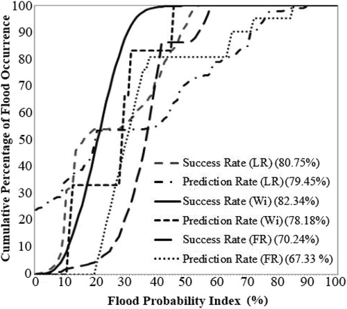
Overall, Wi impressed, outperforming the other methods and producing the most accurate outcomes, although all three models proved to be acceptable for susceptibility mapping in the study area. It can be concluded that Wi displayed the best performance in this study, and the robustness of this method was demonstrated in flood susceptibility modelling and prediction.

6. Conclusion

Flood susceptibility maps are a fundamental step in flood hazard, vulnerability, and risk analysis. Therefore, it is essential to produce the most precise and reliable flood susceptibility maps possible. The application of several statistical methods has previously been tested in flood modelling; however, the Wi method has not been evaluated in this domain. The Wi technique has been found to be easily understandable and cost-effective for mapping landslide prone areas. Hence, the question is whether it would perform at similar levels of precision for flood susceptibility mapping. In the current research, the Wi method was applied, and its outcome was compared with the performance of two popular statistical techniques, FR and LR. The Wi method recognizes the existence of the flooded points in each class of every conditioning factor and assigns weights to them individually. The final flood susceptibility map was produced by combining all of the weight conditioning factors. The validation results from AUC showed that the flood susceptibility maps generated from Wi and LR are more reliable compared to the FR results. The prediction rates were 79.45%, 78.18%, and 67.33% for the LR, Wi, and FR models, respectively. The accuracies indicated that the two models of LR and Wi have almost equal prediction capabilities; however, the Wi method had a higher success rate (82.34%) compared to the 80.75% obtained by the LR method. This shows the superior performance of the Wi method compared to both FR and LR. Flood susceptibility maps have been shown to be of great assistance in properly defining urban expansion and planning strategies. As the outcomes are produced in medium-scale maps, in situ measurements are required in order to have more accurate information about potential flooding regions. However, production of probability maps, such as in this research, can greatly aid in understanding flood risks and probabilities, leading to more preparedness for future flooding events.

Disclosure statement

No potential conflict of interest was reported by the authors.

References

- Aghdam IN, Varzandeh MHM, Pradhan B. 2016. Landslide susceptibility mapping using an ensemble statistical index (Wi) and adaptive neuro-fuzzy inference system (ANFIS) model at Alborz Mountains (Iran). Environ Earth Sci. 75:1–20.
- Anjum MN, Ding Y, Shangguan D, Ijaz MW, Zhang S. 2016. Evaluation of high-resolution satellite-based real-time and post-real-time precipitation estimates during 2010 extreme flood event in Swat River Basin, Hindukush region. Adv Meteorol. 2016:1–8.
- Ayalew L, Yamagishi H. 2005. The application of GIS-based logistic regression for landslide susceptibility mapping in the Kakuda-Yahiko Mountains, Central Japan. Geomo. 65:15–31.
- Ayalew L, Yamagishi H, Ugawa N. 2004. Landslide susceptibility mapping using GIS-based weighted linear combination, the case in Tsugawa area of Agano River, Niigata Prefecture, Japan. Landslides. 1:73–81.
- Bai S, Wang J, Zhang Z, Cheng C. 2012. Combined landslide susceptibility mapping after Wenchuan earthquake at the Zhouqu segment in the Bailongjiang Basin, China. Catena. 99:18–25.
- Bohensky EL, Leitch AM. 2014. Framing the flood: a media analysis of themes of resilience in the 2011 Brisbane flood. Reg Environ Change. 14:475–488.
- Bourenane H, Bouhadad Y, Guettouche MS, Braham M. 2015. GIS-based landslide susceptibility zonation using bivariate statistical and expert approaches in the city of Constantine (Northeast Algeria). Bull Eng Geol Environ.74:337–355.
- Bronstert A. 2003. Floods and climate change: interactions and impacts. Risk Anal. 23:545–557.
- Bui DT, Lofman O, Revhaug I, Dick O. 2011. Landslide susceptibility analysis in the Hoa Binh province of Vietnam using statistical index and logistic regression. Nat Hazards. 59:1413.
- Bui DT, Pradhan B, Nampak H, Bui Q-T, Tran Q-A, Nguyen Q-P. 2016. Hybrid artificial intelligence approach based on neural fuzzy inference model and metaheuristic optimization for flood susceptibility modeling in a high-frequency tropical cyclone area using GIS. J Hydrol. 540:317–330.
- Chang F-J, Tsai M-J. 2016. A nonlinear spatio-temporal lumping of radar rainfall for modeling multi-step-ahead inflow forecasts by data-driven techniques. J Hydrol. 535:256–269.
- Chau K, Wu C, Li Y. 2005. Comparison of several flood forecasting models in Yangtze River. J Hydrol Eng. 10:485–491.
- Chen C-Y, Yu F-C. 2011. Morphometric analysis of debris flows and their source areas using GIS. Geomo. 129:387–397.
- Chen SH, Lin YH, Chang LC, Chang FJ. 2006. The strategy of building a flood forecast model by neuro‐fuzzy network. Hydrol process. 20:1525–1540.
- Chen W, Chai H, Sun X, Wang Q, Ding X, Hong H. 2016. A GIS-based comparative study of frequency ratio, statistical index and weights-of-evidence models in landslide susceptibility mapping. Arab J Geosci. 9:1–16.
- Chen W, Li H, Hou E, Wang S, Wang G, Panahi M, Li T, Peng T, Guo C, Niu C. 2018a. GIS-based groundwater potential analysis using novel ensemble weights-of-evidence with logistic regression and functional tree models. Sci Total Environ. 634:853–867.
- Chen W, Xie X, Peng J, Shahabi H, Hong H, Bui DT, Duan Z, Li S, Zhu A-X. 2018b. GIS-based landslide susceptibility evaluation using a novel hybrid integration approach of bivariate statistical based random forest method. Catena. 164:135–149.
- Chen W, Xie X, Peng J, Wang J, Duan Z, Hong H. 2017. GIS-based landslide susceptibility modelling: a comparative assessment of kernel logistic regression, Naïve-Bayes tree, and alternating decision tree models. Geomat Nat Haz Risk. 8:950–973.
- Chen Y-R, Yeh C-H, Yu B. 2011. Integrated application of the analytic hierarchy process and the geographic information system for flood risk assessment and flood plain management in Taiwan. Nat Hazards. 59:1261–1276.
- Cinderby S, Forrester JM. 2016. Co-designing possible flooding solutions: participatory mapping methods to identify flood management options from a UK borders case study. J Geogr Inf Sci. 1:149–156.
- Dahri N, Abida H. 2017. Monte Carlo simulation-aided analytical hierarchy process (AHP) for flood susceptibility mapping in Gabes Basin (southeastern Tunisia). Environ Earth Sci. 76:302.
- Dang ATN, Kumar L. 2017. Application of remote sensing and GIS-based hydrological modelling for flood risk analysis: a case study of District 8, Ho Chi Minh City, Vietnam. Geomat Nat Haz Risk. 8:1792–1811.
- Dawson CW, Abrahart RJ, Shamseldin AY, Wilby RL. 2006. Flood estimation at ungauged sites using artificial neural networks. J Hydrol. 319:391–409.
- De Risi R. 2013. A probabilistic bi-scale framework for urban flood risk assessment. Naples (Italy): University of Naples Federico II.
- Dempster AP. 2008. A generalization of Bayesian inference. In Kacprzyk J, editor. Classic works of the Dempster-Shafer theory of belief functions. Warsaw (Poland): Springer. p. 73–104.
- Fathzadeh A, Jaydari A, Taghizadeh-Mehrjardi R. 2017. Comparison of different methods for reconstruction of instantaneous peak flow data. Intell Autom Soft Co. 23:41–49.
- Forte F, Strobl R, Pennetta L. 2006. A methodology using GIS, aerial photos and remote sensing for loss estimation and flood vulnerability analysis in the Supersano-Ruffano-Nociglia Graben, southern Italy. Environ Geol. 50:581–594.
- Ghalkhani H, Golian S, Saghafian B, Farokhnia A, Shamseldin A. 2013. Application of surrogate artificial intelligent models for real‐time flood routing. Water Environ J. 27:535–548.
- Gómez-Palacios D, Torres MA, Reinoso E. 2017. Flood mapping through principal component analysis of multitemporal satellite imagery considering the alteration of water spectral properties due to turbidity conditions. Geomat Nat Haz Risk. 8:607–623.
- Güçlü YS, Şen Z. 2016. Hydrograph estimation with fuzzy chain model. J Hydrol. 538:587–597.
- Hong Y-ST, White PA. 2009. Hydrological modeling using a dynamic neuro-fuzzy system with on-line and local learning algorithm. Adv Water Resour. 32:110–119.
- Hostache R, Chini M, Matgen P, Giustarini L. 2013. A new automatic SAR-based flood mapping application hosted on the European Space Agency’s grid processing on demand fast access to imagery environment. Proc EGU General Assembly Conference Abstracts. 15:1–5.
- Jaafari A, Najafi A, Pourghasemi H, Rezaeian J, Sattarian A. 2014. GIS-based frequency ratio and index of entropy models for landslide susceptibility assessment in the Caspian forest, northern Iran. Int J Environ Sci Technol. 11:909–926.
- Jayakrishnan R, Srinivasan R, Santhi C, Arnold J. 2005. Advances in the application of the SWAT model for water resources management. Hydrol Process. 19:749–762.
- Jebur MN, Pradhan B, Tehrany MS. 2014. Optimization of landslide conditioning factors using very high-resolution airborne laser scanning (LiDAR) data at catchment scale. Remote Sens Environ. 152:150–165.
- Jothibasu A, Anbazhagan S. 2016. Flood susceptibility appraisal in Ponnaiyar River Basin, India using frequency ratio (FR) and Shannon’s Entropy (SE) models. Int J Adv Rem Sens GIS 5:1946–1962.
- Juarez-Lucas AM, Kibler KM, Ohara M, Sayama T. 2016. Benefits of flood-prone land use and the role of coping capacity, Candaba floodplains, Philippines. Nat Hazards. 84:2243–2264.
- Kang P, Zhang L. 2016. Logistic regression modeling for the length of stay among the hospitalized patients after the 2010 Yushu earthquake. In: Zhang L, editor. Modeling the injury flow and treatment after major earthquakes. Dordrecht: Springer. p. 41–56.
- Karimi F, Sultana S, Shirzadi Babakan A, Royall D. 2018. Land suitability evaluation for organic agriculture of wheat using GIS and multicriteria analysis. Appl Geogr. 10:1–17.
- Kassa BA. 2014. Assessing the main causes of flood hazard through examining Gis and Rs based Land Use Land Cover (Lulc) change, topography (slope) and drainage density analysis in Alamata Woreda, Southern Tigray Zone, Ethiopia. AJSSH. 4:270–290.
- Khosravi K, Nohani E, Maroufinia E, Pourghasemi HR. 2016. A GIS-based flood susceptibility assessment and its mapping in Iran: a comparison between frequency ratio and weights-of-evidence bivariate statistical models with multi-criteria decision-making technique. Nat Hazards. 83:1–41.
- Khosravi K, Pham BT, Chapi K, Shirzadi A, Shahabi H, Revhaug I, Prakash I, Bui DT. 2018. A comparative assessment of decision trees algorithms for flash flood susceptibility modeling at Haraz watershed, northern Iran. Sci Total Environ. 627:744–755.
- Khosrokhani M, Pradhan B. 2014. Spatio-temporal assessment of soil erosion at Kuala Lumpur metropolitan city using remote sensing data and GIS. Geomat Nat Haz Risk. 5:252–270.
- Kia MB, Pirasteh S, Pradhan B, Mahmud AR, Sulaiman WNA, Moradi A. 2012. An artificial neural network model for flood simulation using GIS: Johor River Basin, Malaysia. Environ Earth Sci. 67:251–264.
- Kim KD, Lee S, Oh HJ, Choi JK, Won JS. 2006. Assessment of ground subsidence hazard near an abandoned underground coal mine using GIS. Environ Geol. 50:1183–1191.
- Kjeldsen TR. 2010. Modelling the impact of urbanization on flood frequency relationships in the UK. Hydrol Res. 41:391–405.
- Lee M-J, Kang J-e, Jeon S. 2012. Application of frequency ratio model and validation for predictive flooded area susceptibility mapping using GIS. Proceedings of the Geoscience and Remote Sensing Symposium (IGARSS), Jul 22–27; Munich (Germany): IEEE International. p. 4.
- Lee S. 2005. Application of logistic regression model and its validation for landslide susceptibility mapping using GIS and remote sensing data. Int J Remote Sens. 26:1477–1491.
- Lee S, Pradhan B. 2006. Probabilistic landslide hazards and risk mapping on Penang Island, Malaysia. J Earth Sys Sci. 115:661–672.
- Li L, Lan H, Guo C, Zhang Y, Li Q, Wu Y. 2016. A modified frequency ratio method for landslide susceptibility assessment. Landslides. 14:727–741.
- Liao X, Carin L. 2009. Migratory logistic regression for learning concept drift between two data sets with application to UXO sensing. IEEE Trans Geosci Remote Sens. 47:1454–1466.
- Liong SY, Sivapragasam C. 2002. Flood stage forecasting with support vector machines. Singapore: Wiley Online Library.
- Liu Y, De Smedt F. 2004. WetSpa extension, a GIS-based hydrologic model for flood prediction and watershed management. Brussel (Belgium):Vrije Universiteit Brussel. p. 1–108.
- Maier HR, Dandy GC. 2000. Neural networks for the prediction and forecasting of water resources variables: a review of modelling issues and applications. Environ Modell Softw. 15:101–124.
- Manap MA, Nampak H, Pradhan B, Lee S, Sulaiman WNA, Ramli MF. 2014. Application of probabilistic-based frequency ratio model in groundwater potential mapping using remote sensing data and GIS. Arab J Geosci. 7:711–724.
- Mathew J, Jha V, Rawat G. 2009. Landslide susceptibility zonation mapping and its validation in part of Garhwal Lesser Himalaya, India, using binary logistic regression analysis and receiver operating characteristic curve method. Landslides. 6:17–26.
- Merz B, Thieken A, Gocht M. 2007. Flood risk mapping at the local scale: concepts and challenges. In: Begum S, Stive MJF, Hall JW, editors. Flood risk management in Europe Unital. Dordrecht (Nether Land): Springer. p. 231–251.
- Mojaddadi H, Pradhan B, Nampak H, Ahmad N, Ghazali AH. 2017. Ensemble machine-learning-based geospatial approach for flood risk assessment using multi-sensor remote-sensing data and GIS. Geomat Nat Haz Risk. 8:1080–1102.
- Nandi A, Mandal A, Wilson M, Smith D. 2016. Flood hazard mapping in Jamaica using principal component analysis and logistic regression. Environ Earth Sci. 75:1–16.
- Nefeslioglu H, Sezer E, Gokceoglu C, Bozkir A, Duman T. 2010. Assessment of landslide susceptibility by decision trees in the metropolitan area of Istanbul, Turkey. Math Probl Eng. 1:1–15.
- Novelo-Casanova DA, Rodríguez-Vangort F. 2016. Flood risk assessment. Case of study: Motozintla de Mendoza, Chiapas, Mexico. Geomat Nat Haz Risk. 7:1538–1556.
- Nurmohamed R, Naipal S, De Smedt F. 2012. Hydrologic modeling of the Upper Suriname River basin using WetSpa and ArcView GIS. JOSH. 6:1–17.
- Pourghasemi HR, Pradhan B, Gokceoglu C. 2012. Application of fuzzy logic and analytical hierarchy process (AHP) to landslide susceptibility mapping at Haraz watershed, Iran. Nat Hazards. 63:965–996.
- Pradhan B. 2009. Groundwater potential zonation for basaltic watersheds using satellite remote sensing data and GIS techniques. Open Geosci. 1:120–129.
- Pradhan B. 2010. Flood susceptible mapping and risk area delineation using logistic regression, GIS and remote sensing. JOSH. 9:1–18.
- Pradhan B, Tehrany MS, Jebur MN. 2016. A new semiautomated detection mapping of flood extent from TerraSAR-X satellite image using rule-based classification and Taguchi optimization techniques. IEEE Trans Geosci Remote Sens. 54:4331–4342.
- Pradhan B, Youssef A. 2011. A 100‐year maximum flood susceptibility mapping using integrated hydrological and hydrodynamic models: Kelantan River Corridor, Malaysia. J Flood Risk Manag. 4:189–202.
- Queensland Floods Commission of Inquiry (QFCI) (2012). Queensland Floods Commission of Inquiry: Final Report. Inquiry, QFCo, & Holmes, CE.
- Rahmati O, Pourghasemi HR, Zeinivand H. 2016. Flood susceptibility mapping using frequency ratio and weights-of-evidence models in the Golastan Province, Iran. Geocarto Int. 31:42–70.
- Regmi AD, Devkota KC, Yoshida K, Pradhan B, Pourghasemi HR, Kumamoto T, Akgun A. 2014. Application of frequency ratio, statistical index, and weights-of-evidence models and their comparison in landslide susceptibility mapping in Central Nepal Himalaya. Arab J Geosci. 7:725–742.
- Shabani F, Kumar L, Esmaeili A. 2014. Improvement to the prediction of the USLE K factor. Geomorphology. 204:229–234.
- Shabani F, Shafapour TM, Solhjouy-Fard S, Kumar L. 2018. A comparative modeling study on non-climatic and climatic risk assessment on Asian Tiger Mosquito (Aedes albopictus). Peer J. 6:e4474. doi: 10.7717/peerj.4474.
- Sahoo G, Schladow S, Reuter J. 2009. Forecasting stream water temperature using regression analysis, artificial neural network, and chaotic non-linear dynamic models. J Hydrol. 378:325–342.
- Shafer G. 1976. A mathematical theory of evidence. New Jersey (US): Princeton University Press.
- Shrestha RR, Nestmann F. 2009. Physically based and data-driven models and propagation of input uncertainties in river flood prediction. J Hydrol Eng. 14:1309–1319.
- Stefanidis S, Stathis D. 2013. Assessment of flood hazard based on natural and anthropogenic factors using analytic hierarchy process (AHP). Nat Hazards. 68:569–585.
- Sun D, Yu Y, Goldberg MD. 2011. Deriving water fraction and flood maps from MODIS images using a decision tree approach. J Sel Topics Appl Earth Observ Remote Sens. 4:814–825.
- Tehrany M, Jones S. 2017. Evaluating the variations in the flood susceptibility maps accuracies due to the alterations in the type and extent of the flood inventory. ISPRS-Int Arc Photogramm, Remote Sens Spatial Inform Sci. 12:209–214.
- Tehrany MS, Lee M-J, Pradhan B, Jebur MN, Lee S. 2014a. Flood susceptibility mapping using integrated bivariate and multivariate statistical models. Environ Earth Sci. 72:4001–4015.
- Tehrany MS, Pradhan B, Jebur MN. 2013. Spatial prediction of flood susceptible areas using rule based decision tree (DT) and a novel ensemble bivariate and multivariate statistical models in GIS. J Hydrol. 504:69–79.
- Tehrany MS, Pradhan B, Jebur MN. 2014b. Flood susceptibility mapping using a novel ensemble weights-of-evidence and support vector machine models in GIS. J Hydrol. 512:332–343.
- Tehrany MS, Pradhan B, Jebur MN. 2015a. Flood susceptibility analysis and its verification using a novel ensemble support vector machine and frequency ratio method. Stoch Environmen Res Risk Assess. 29:1149–1165.
- Tehrany MS, Pradhan B, Mansor S, Ahmad N. 2015b. Flood susceptibility assessment using GIS-based support vector machine model with different kernel types. Catena. 125:91–101.
- Tehrany MS, Shabani F, Javier DN and Kumar L. 2017. Soil erosion susceptibility mapping for current and 2100 climate conditions using evidential belief function and frequency ratio. Geomatics Natural Hazards and Risk. 1–21.
- Tehrany MS, Shabani F, Neamah Jebur M, Hong H, Chen W, Xie X. 2017. GIS-based spatial prediction of flood prone areas using standalone frequency ratio, logistic regression, weight of evidence and their ensemble techniques. Geomat Nat Haz Risk. 8:1538–1561.
- Tien Bui D, Le K-TT, Nguyen VC, Le HD, Revhaug I. 2016. Tropical forest fire susceptibility mapping at the Cat Ba National Park Area, Hai Phong City, Vietnam, using GIS-Based kernel logistic regression. Remote Sens. 8:347.
- Umar Z, Pradhan B, Ahmad A, Jebur MN, Tehrany MS. 2014. Earthquake induced landslide susceptibility mapping using an integrated ensemble frequency ratio and logistic regression models in West Sumatera Province, Indonesia. Catena. 118:124–135.
- Werner M, Hunter N, Bates P. 2005. Identifiability of distributed floodplain roughness values in flood extent estimation. J Hydrol. 314:139–157.
- Xiong Y, Zuo R. 2018. GIS-based rare events logistic regression for mineral prospectivity mapping. Comput Geosci. 111:18–25.
- Yalcin A. 2008. GIS-based landslide susceptibility mapping using analytical hierarchy process and bivariate statistics in Ardesen (Turkey): comparisons of results and confirmations. Catena. 72:1–12.
- Yilmaz I. 2009. Landslide susceptibility mapping using frequency ratio, logistic regression, artificial neural networks and their comparison: a case study from Kat landslides (Tokat–Turkey). Comput Geosci. 35:1125–1138.
- Youssef AM, Pradhan B, Sefry SA. 2016. Flash flood susceptibility assessment in Jeddah city (Kingdom of Saudi Arabia) using bivariate and multivariate statistical models. Environ Earth Sci. 7:149–161.
- Yusoff S, Pradhan B, Manap MA, Shafri HZM. 2015. Regional gold potential mapping in Kelantan (Malaysia) using probabilistic based models and GIS. Open Geosci. 7:149–161.
- Zhang M, Cao X, Peng L, Niu R. 2016. Landslide susceptibility mapping based on global and local logistic regression models in Three Gorges Reservoir area, China. Environ Earth Sci. 75:1–11.