A neural network model applied to landslide susceptibility analysis (Capitanejo, Colombia)

Abstract

The generation of landslide present in the municipality of Capitanejo (Santander-Colombia) is conditioned to lithological, structural and morphometric factors that are related to the climatic activity. These factors describe a pattern of instability in the rocks, which generates falls, slides and flows. These conditions are seen in the results of a neural network model generated with the backpropagation algorithm. This model presented the conditions of the study area evaluated by the degree of susceptibility to landslide. The model predicted 92.86% of the data that were not entered in the learning module, which represents 50% of the landslides mapped in the region. This simulation generates different levels of susceptibility to landslide from very low to very high. In the study area, a tendency for moderate to very high susceptibility to landslides was found for the margins of the Chicamocha river valley. In turn, this area presents the largest number of active processes (falls and flows), which generates a problem that affects several levels within the sectors of production, communication and infrastructure of the community of Capitanejo.

Keywords:

• Susceptibility model
• landslide simulation
• neural network
• Capitanejo

1. Introduction

The estimation of susceptibility by landslide allows to determine sectors within the relief that are unstable to processes where the geological, geomorphological and climatic activities of a region interact. In recent decades, these instability conditions on the slopes resulting from the above processes have been the subject of research in various branches of the science of geology. These investigations focus on how to interpret the evolution and behaviour of these active processes from various points of view (Carrara et al. 1991). The form of evaluation and prediction has been a subject of great interest, requiring the integration of an interdisciplinary approach (Aleotti and Chowdhury 1999). These natural processes are reconstructed to determine their physical qualities and thus understand the variables intervening in their generation (Chacon et al. 2006). Now, his interpretation is united by the interaction that man has generated in his environment. An example of this is the way in which new areas are conquered by processes of deforestation for anthropic activities that have caused an increase in soil erosion and sediment transport, resulting in the degradation of soils that can generate floods or landslide (Bathrellos et al. 2017). The evaluation of these factors contributes in the construction of guidelines or basic aspects in the territorial planning, generating in this way a baseline in the expansion of anthropic projects (Bathrellos et al. 2012). In turn, projections are made in different scenarios, where the conditions of the study region are simulated under statistical or mathematical parameters to predict the zones with possible events similar to those evaluated (Ayala 1987; Martinez-Graña et al. 2014). The development of this type of research is considered due to its transcending character in social aspects (Ayala-Carcedo and Cantos 2002; Martinez-Graña et al. 2013). Globally, this problem has had consequences in regions with urban expansion or anthropogenic activities, especially in equatorial áreas (Alcantara-Ayala 2002).

For Colombia these factors in the last decades have manifested themselves more frequently, with high mountainous zones being those that present/display more recorded events (Cardona et al. 2004). Regions such as Antioquia, Caldas, Tolima, Santander and Cundinamarca had high rates of landslides in 2002 (INGEOMINAS 2002). In 2010 this rate increased due to the gradual change of the climatic conditions, affecting 506,825 people as a result of hillside movement events (CEPAL 2012). In the study region, these events occur more frequently due to both climatic and geological factors as well as human activity. These factors are considered important as they cause an increase in active processes due to the action generated by the progressive weakening of the mechanical properties of the rocks that cause weathering and erosion of the constant form (Costa and Baker 1981; Soeters and Van Westen 1996). These factors are modeled by means of mathematical methods that relate to the variables that intervene in the generation of the event. Their construction is performed depending on the availability, quality and accuracy of data, the resolution of the information, the required results, and the work scale (Soeters and Van Westen 1996). Within these parameters we have the heuristic, statistical, deterministic and stochastic methods, the latter being the method that will be used in the study area for its versatility in how to evaluate each of the variables in a random way and the degree of pressure of the simulation with respect to the work scale.

Stochastic methods take variables as random data, which are related to each other with probabilistic functions (Gardiner 1985). These relationships are determined depending on the variables entered, taking into account the geological and geomorphological factors in this study. The correlation of the data effects occurs within a mathematical model that simulates the possible events of landslide from the information entered. The implementation of the stochastic method involves the execution of an algorithm that correlates these variables. The algorithms most implemented for this type of problems are: fuzzy logic (FL), fuzzy algorithms (FA), artificial neural networks (ANN), genetic algorithms (GA), geotechnical programming (GP), and ant colony and evolved algorithms (Pistocchi et al. 2002; Akgun 2012). Slope movement susceptibility analysis is performed under the algorithm of neural networks; its implementation is based on the way the variables are processed within the algorithm due to its adaptive learning, self-organization, fault tolerance and time operation. Neural Networks are defined as mass and parallel interconnections of simple elements with a hierarchical organization (Matich 2001).

The organization of these data is established by logical functions, where the variables entered interact to generate a mathematical simulation of the problem, a condition based on how the human brain interacts in problem solving. From this simulation, the areas susceptible to landslide by active processes are determined, evaluated on a scale from very low (without affectation) to very high (with affectation). There are conditions that represent a disadvantage with respect to the quality of life of a region, and that is reflected in the area of study because it involves elements such as housing, road network and agricultural activity. The implementation of this type of mathematical models in the simulation of landslide events based on variables obtained from geology, geomorphology and digital terrain models are the objective in the assessment of areas predisposed to these events. These conditions are the object of the present research work, where we want to establish and delimit the zones that the mathematical model “Neural Network” establish as possible regions that generate landslide. Based on the results obtained, studies and policies can be established in greater detail within the territorial planning plans for areas with regions that are more susceptible to landslide.

2. Geological and geomorphological context

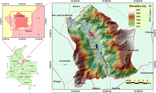
The study region belongs to the municipality of Capitanejo, Santander, and is located north of Bogota, Capital of Colombia (Figure 1). It has an extension of 205 km² and is crossed by the Chicamocha River and valley. The municipality of Capitanejo has a strong topographical contrast (slopes between 0° and 80°, with a predominance of slope >45°) and elevation of between 1,100 m and 3,397 m. The climatic factor is controlled by conditions of the Intertropical Convergence Zone (ITCZ), characterized by a wide belt of low pressure constituted by currents of upward air, where large masses of warm and humid air converge from the north and south of the Intertropical Zone. The accumulated rainfall presents an annual average of 950 mm, in a regime of bimodal rains, between the months of March and April and again in August and September. Average temperatures range from 16 °C to 28 °C (IDEAM 2016).

Figure 1. Geographic location of the study area.

2.1. Geological and geomorphological context

The study area is located in one of three orogenic systems present in Colombia called the Cordillera Oriental. It is characterized as being an orogenic system with high tectonic and structural complexity, which developed in the NE–SE direction. This orogenic event initiated its main phase of rising after the Middle Miocene by reactivation and tectonic inversion of normal faults of old extensional basins of the Upper Jurassic and Lower Cretaceous (Van der Hammen 1958; Cooper et al. 1995).

With the lifting of the eastern mountain chain, a series of rocks was created on the surface of the study region (units are described in the geological memory of topographic map number 136, Vargas et al. 1976; Figure 2a). They began with a Pre-Devonian-age metamorphic basement (PD1, the letter indicates the geological period and the number the chronostratigraphic position), with lithology of quartzmonzonítico and granodiorítico gneiss; tonalitic and diorite gneiss of igneous origin. The Devonian age (Df2, Df3, Df4) presented with wall to top shales, conglomerates, black claystones and sandstones. The shales were subjected to contact metamorphism, producing phyllitas, argillite, and gray marbles. During the Permian (Pf5) age there was a deposition of siltstone and mudstone with calcareous nodules, shales, and alternation of mudstones and conglomerates.

Figure 2. Geological map (a), adapted from the geological map scale 1:100,000 (Vargas et al., 1976) and a morphogenetic map (b).

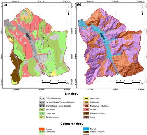
Superimposed on this sequence, in the lower Cretaceous there was an alternation of the appearance of biomicritic limestones, mudstones and sandstones. In the upper Cretaceous (Kf6), a sedimentary sequence was deposited, which began with clay-limestones, calcareous shales, dark gray shales and limestone concretions with fossils. Superimposed on this sequence is fossiliferous mudstone, which is slightly calcareous, and thin layers of mudstone interspersed with carbon. Finally, at the end of the Cretaceous (Kf7, Kf8) there were black shales with sandy intercalations towards the base and banks of fossiliferous limestones deposited towards the ceiling. During the Paleogene (Tf9), quartz sandstones were deposited with alternations of carbonate mudstone and mudstone, quartz and feldspathic sandstones, with small intercalations of carbonaceous mudstone and layers of carbon. During the Quaternary (Q10, Q11, Q12), different forms of deposits were generated, such as dejection cones and alluvial fans, fluvial terraces and ‘hillside deposits’ or ‘colluvion’ (Vargas et al. 1976).

The structural behaviour of the area is very complex and is conditioned by the Bucaramanga–Santa Marta fault passing through the study area on the west bank, which is characterized by a fault direction of N340°E with a sinistral movement, and an estimated of strike-slip displacement of between 40 and 240 km on a 12-km deep detachment (Campbell 1965; Toro 1990; Leon 1991). The vertical displacement allows for the interpretation in some sectors of movements of inverse type with dips towards the east (low to high angle), and in their extreme south, rides (Julivert and Tellez 1961; Boinet et al. 1989; Cediel et al. 2003). In turn, the study area is crossed by the fault of the Chicamocha that is characterized by a rectilinear trace that comes into contact with Cretaceous sediments, as well as high-angle inverse type faults that mostly correspond to N-S direction fractures, as well as anticlinical and synclinal folds (Vargas et al. 1976).

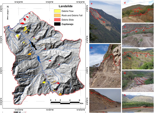
Geomorphologically, the region shows strong conditions with respect to the structural units (40%) such as hillsides, ridges, hills and structural hills that are caused by the action of the Bucaramanga - Santa Marta and Chicamocha faults that result in an abrupt topographic contrast of the current slope of high relief that also generates strong erosive processes, giving rise to erosive and gravity-type units (40%) such as slopes with surface erosion (gullies and furrows), as well as ridges and denuded hills (Figure 2b). These events are described through their relation to all the slope movements of a mass of rock, debris or earth due to the the effects of gravity (Cruden 1991). Within the gravitational units, there are rock fall (9 events), debris fall (12 events), debris slide (21 events), debris flow (10 events), and creep (2 events) classified according to Cruden and Varnes (1996). The morphodynamics of the region show a total of 54 landslide events. The information taken from the National System of Mass Movements database (SIMMA 2017) showed nine landslides, while the other movements were obtained by photointerpretation of the study area (45 landslides) (Figure 3). Due to interaction of climatic factors in the region and the units of structural and erosive type, are developed towards the areas of moderate to low slopes, geomorphological units of fluvial origin 151 (20%) product of the degradation and movement of the particles, and that they comprise the river deposits. These fluvial type units originate different orders of terraces, plans and flood plains, as well as dejection cones and alluvial fans.

Figure 3. Hillside movements in the study area. Debris slide (a, d, e and f), rock and debris fall (b and c), creep (g), and lateral undercutting (h), products of the course of the channel of Chicamocha River (Provided by Jorge Leonardo Chaparro).

3. Database and analysis

The analysis of the susceptibility by landslide is established in several stages described in Figure 4. This susceptibility is described by its relation to something that has not yet occurred and is usually defined as the ease with which a phenomenon can occur based on local conditions (Suarez 2009). Applied to landslide, this analysis generates an estimate of a region in which landslides exist or may occur (Fell et al. 2008; Suarez 2009). The origin of the instability processes of the existing slopes in the study region is controlled by aspects such as the tectonic configuration, high slopes, seismic activity and climatic factors, with the Department of Santander being one of the regions with the largest number of events recorded (INGEOMINAS 2002).

Figure 4. Methodological flow for landslide susceptibility. SPI: stream power index; TWI: topographic wetness index; SGC: servicio geologico colombiano; DEM: digital elevation model.

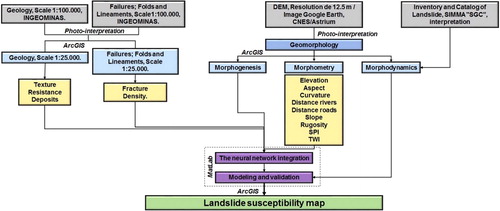
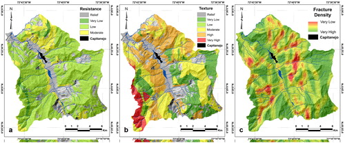
Within the aspects that were taken to evaluate the susceptibility for landslide in the region, one is the geology, which plays a very important role in this analysis of landslide susceptibility, since lithological and structural conditions can be sources of instability (e.g. this are shales for the study area, which present the greatest amount of landslide; Ohlmacher 2000). The type of rock and the deformation that it can present are very influential factors, as the resistance, texture and degree of fracturing are a focus of instability on the slopes, especially in shale, limestone and sandstone (Figure 5) Resistance is a variable that influences the susceptibility of the rocks due to their character of fracture and is interpreted according to the capacity for resisting compressive stresses, shear stresses, and other stresses. It is classified according to the performed analyses by Hoek and Brown (1997) The characteristic of texture reflects the internal structure of the rocks that refers to the arrangement of particles, groups of particles and empty spaces, depending on this relationship the degree of susceptibility according to their condition is quantified. Categories include massive crystalline, banded crystalline, cemented clastic, consolidated clastic, folded crystalline and rocks of fault. The fracturing density represents the degree of fracturing of the rocks when moving away from the structures that generate deformation in the terrain (faults and folds). It is evaluated by calculating the density of lines in the vicinity of each pixel defined by a search radius. It ranks from very low to very high according to the degree of activity in rocks (UNESCO 1976; Matula 1981; Martinez-Graña et al. 2016). Geomorphology is evaluated in terms of morphogenetic, morphodynamic and morphometric factors (the first are two described above) (Martinez-Graña et al. 2014). These factors were obtained by integrating conditions that relate geology, topography, satellite imagery, the digital elevation model (DEM), and active process logging. The DEM was created by the Japan Aerospace Exploration Agency (JAXA) with spatial resolution of 12.5 m. The data set has a elevation variation between 1,011 and 3,397 m and a slope angle between 0° and 78.3° (ASF 2016).

Figure 5. Classification of lithology depending on resistance (a), texture (b) and fracture density (c).

Morphometric factors are constructed from the variables obtained from the DEM and topography (Pike 1995); these variables are selected for their influence on the instability processes of the slopes in the study region (Gallant and Hutchinson 2008; Olaya 2009). The variables processed from the DEM are elevation, aspect, curvature, slope, rugosity, the stream power index (SPI) and topographic wetness index (TWI) and topography distance to rivers and the distance to the roads.

The elevation conditions the relief and influences the erosive processes as a consequence of the uprising of the mountains, an effect that is evaluated from the base level (Ercanoglu and Gokceoglu 2002; Ayalew and Yamagishi 2005; Nefeslioglu et al. 2010; Akgun et al. 2012a; Akgun et al. 2012b; Botzen et al. 2013). This factor has an influence on landslides between the heights of 1,200 and 1,400 that have high slopes. The elevation value was also used for the SPI and TWI factors, where it is taken as a topographic value combined with the natural slope of the terrain (Figure 6a).

Figure 6. Morphometric variables. Elevation (a), aspect (b), curvature (c), distance to rivers (d), distance to roads (e), slope (f), rugosity (g), SPI (h) and TWI (i).

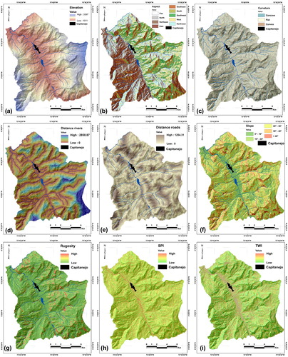
The aspect shows the layout of the slopes with reference to their geographical sense (Saha et al. 2005; Yalcin et al. 2011). Aspect is evaluated in the study region because of its relation with other factors such as rainfall, amount of solar brightness, and morphogenesis, factors that increase the instability of slopes with a southeast location (Figure 6b). The curvature describes the physical characteristics of the relief, and is associated with concave, convex or straight slope regions (Lee et al. 2004; ESRI 2017), with straight and concave regions registering the greatest number of landslides. The curvature value was also used for the SPI and TWI factors (Figure 6c).

The distance to the rivers is a factor that can negatively affect the stability of the slope in the hillside movements. Close proximity to drainage affects erosive processes due to the effect of the water in the slope of the terrain, generating instability and an increase in water level on plugging the flow (Gokceoglu and Aksoy 1996). This condition is evident within a 500 m perimeter around the banks of the Chicamocha and Servita rivers, as well as in some of their tributary tributaries. This variable was constructed with the Distance tool of ArcMap, taking as main input, the cartographic base of the region, in the same way this procedure is done for the distance attribute to roads (Figure 6d). The distance to the roads of communication is another factor that generates instability in the slopes. Generating a road results in lost natural stability, for which compensation may occur through strong erosive processes on the exposed slope to balance the system (Ayalew and Yamagishi 2005). This effect is observed throughout the main route of the municipality of Capitanejo, as well as in some alternate routes within the rural hull (Figure 6e).

The slope evaluates the relationship between the degree of inclination of the slopes and the type of rock. This relationship is given by the angle of friction, permeability and cohesion between particles (Saha et al. 2005; Yalcin et al. 2011). The northern region of the municipality of Capitanejo is an area very prone to this type of process due to slopes between 20° and 40° (Figure 6f). The rugosity evaluates the conditions of the terrain and its variability. These conditions are established by integrated orientation and slope parameters that determine the vector coefficients in the three axes of the surfaces (Felicisimo 1994). This aspect has little influence on the processes of generation of landslide, but it does have a strong influence on the erosion control of these surfaces that are evaluated by the SPI and TWI parameters (Figure 6g).

The stream power index (SPI) measures the erosive power of the streams and is considered a conditioning factor for slope stability (Regmi et al. 2014). The incidence of this factor presents flow conditions with a moderate degree of erosion, an aspect that is associated with the abrupt changes of the topography and the high slopes (Figure 6h). It is defined by the Equation (1)(1) $$\text{SPI}: \text{As}\times \text{tang}$$(1) , where As is the specific catchment area in metres and σ is the slope angle in degrees. (1) $$\text{SPI}: \text{As}\times \text{tang}$$(1)

The topographic wetness index (TWI) represents another important topographic factor within the morphometric conditions of the terrain, as it evaluates the cumulative flow rate point-to-point upstream with the slope angle of each runway (Poudyal et al. 2010; Figure 6i). The TWI parameter is calculated by the Equation (2)(2) $$\text{TWI}:\hspace{0.17em}\text{ln}\left(\text{As}/\text{tang}\right)$$(2) , where As is the specific catchment area (m) and σ is the slope angle (degs.).The relationship of these variables to landslide present in the region is described in Table 1. (2) $$\text{TWI}:\hspace{0.17em}\text{ln}\left(\text{As}/\text{tang}\right)$$(2)

Table 1. Factors evaluated and representation in the area.

Factor	Class	Without Landslide		With Landslide
		N° Pixel	%	N° de Pixel	%
Lithology	Colluvial Deposits	173643	13.2	561	2.92
	Fan and Alluvial Terraces Deposits	31934	2.4	30	0.16
	Channels and Plains Deposits	87631	6.7	885	4.61
	Sandstone	348614	26.5	4321	22.52
	Limestones	252447	19.2	4688	24.43
	Conglomerates	7555	0.6	–	–
	Limolites	14898	1.1	654	3.41
	Lodolites	21404	1.6	265	1.38
	Lodolites - Phillities	4317	0.3	–	–
	Shales	288400	21.9	7782	40.56
	Marble - Phillite	63534	4.8	–	–
	Gneis	20137	1.5	–	–
Fracture Density	Very Low	461751	35.1	8041	41.91
	Low	488194	37.1	5889	30.69
	Moderate	164399	12.5	4109	21.42
	High	154706	11.8	957	4.99
	Very High	45472	3.5	190	0.99
Morphodynamic	Falls	–	–	4093	21.33
	Slide Rotational	–	–	2382	12.42
	Slide Translational	–	–	5013	26.13
	Flows	–	–	7698	40.12
Elevation	1011–1231	174602	13.28	2706	14.10
	1231–1409	159090	12.10	8869	46.23
	1409–1586	167606	12.75	4791	24.97
	1586–1768	160292	12.19	1750	9.12
	1768–1956	159132	12.11	791	4.12
	1956–2158	153181	11.65	279	1.45
	2158–2367	129463	9.85	–	–
	2367–3397	211171	16.06	–	–
Aspect	Flat	9689	0.74	11	0.06
	North	84379	6.42	1784	9.30
	Northeast	168169	12.79	1067	5.56
	East	155402	11.82	2770	14.44
	Southeast	129955	9.89	1217	6.34
	South	133783	10.18	2498	13.02
	Southwest	192669	14.66	4485	23.38
	West	209499	15.94	3302	17.21
	Norhtwest	230992	17.57	2052	10.70
Curvature	Concave	295973	22.52	5789	30.17
	Flat	725435	55.19	9110	47.48
	Convex	293129	22.30	4287	22.34
Distance Rivers	0–125.62 m	283777	21.59	4808	25.06
	125.62–257.69 m	253537	19.29	3878	20.21
	257.69–400.19 m	225018	17.12	3109	16.20
	400.19–551.27 m	181877	13.84	3018	15.73
	551.27–716.43 m	143921	10.95	2004	10.45
	716.43–907.77 m	106441	8.10	1655	8.63
	907.77–1160.61 m	62677	4.77	515	2.68
	1160.61–1517.91 m	30467	2.32	–	–
	1517.91–1983.88 m	18969	1.44	120	0.63
	1983.88–2858.86 m	7853	0.60	94	0.49
Distance Roads	0–72.88 m	264574	20.13	1521	7.93
	72.88–152.58 m	234830	17.86	1461	7.61
	152.58–233.51 m	188751	14.36	1505	7.84
	233.51–318.68 m	167863	12.77	2138	11.14
	318.68–408.69 m	135383	10.30	2155	11.23
	408.69–506.51 m	111254	8.46	2390	12.46
	506.51–617.58 m	83874	6.38	2450	12.77
	617.58–744.35 m	60784	4.62	2105	10.97
	744.35–894.86 m	42745	3.25	1785	9.30
	894.86–1254.30 m	24479	1.86	1691	8.81
Slope	0°–10°	196354	14.94	526	2.74
	10°–20°	407942	31.03	3044	15.87
	20°–30°	407933	31.03	6169	32.15
	30°–40°	224448	17.07	6082	31.70
	> 40°	77860	5.92	3365	17.54
Rugosity	Low	1111119	84.53	13765	71.75
	Moderate	170203	12.95	4202	21.90
	High	25870	1.97	1211	6.31
TWI	low	413392	31.45	11476	59.81
	Moderate	464844	35.36	6223	32.44
	High	232418	17.68	1487	7.75
SPI	Low	395850	30.11	5482	28.57
	Moderate	652609	49.65	9981	52.02
	High	266078	20.24	3738	19.48

4. Creation of the artificial neural network (ANN) and results

The analysis of the susceptibility is generated by grouping the 14 variables created from the attributes of geology and geomorphology; this process is done by integrating all the inputs in a calculation matrix under a processing module, where, on the one hand, the variables are generated and on the other, there is data for learning. Analysis is carried out using the neural network (ANN), being an information processing system that allows for the solution of complex problems of classification, functional estimation and optimization through the estimation of a linear or nonlinear relationship between the input and output data (Simpson 1990; Anderson and McNeill 1992; De Brio and Sanz 2007).

This analysis requires three steps. Firstly, there is the generation of a database with the created factors of geology and geomorphology. Secondly, there is the creation of the matrices (input, target and sample) and the lastly, there is the establishment of training parameters for the simulation within the ANN. The database is composed of the following variables: resistance, texture, surface formations, fracture density, morphogenetic, elevation, aspect, curvature, distance to rivers, distance to roads, slope, rugosity, SPI, TWI and landslide (50% for training). These data were taken randomly so as not to establish a predisposition in the calculation performed by the ANN (Figure 7).

Figure 7. Processing structure of the ANN.

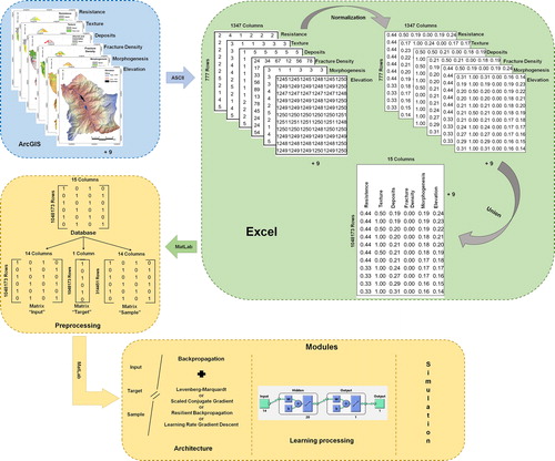
The database is built by importing each variable that is in raster format to ASCII format to be read in a spreadsheet (Excel). The imported variables are presented as individual files (15 files). Their numerical range presents different intervals, this being a problem for the simulation because the neural network looks for patterns within the variables. This is solved by performing a normalization, where values are in a range of [0,1] using Equation (1)(1) $$\text{SPI}: \text{As}\times \text{tang}$$(1) . The value of each cell (Xcell) is subtracted from the minimum value (Xmin) present in the data of the file divided by the result of the maximum value (Xmax) less the minimum value (Xmin) of the file. The information from each standard file is integrated into a single database to be processed in the MatLab R2015a software (Eq. 3(3) $$X´=\frac{X_{\mathit{\text{Celda}}}-X_{\mathit{\text{Min}}}}{X_{\mathit{\text{Max}}}-X_{\mathit{\text{Min}}}},$$(3) ). (3) $$X´=\frac{X_{\mathit{\text{Celda}}}-X_{\mathit{\text{Min}}}}{X_{\mathit{\text{Max}}}-X_{\mathit{\text{Min}}}},$$(3)

The matrices are created from the normalized database inside MatLab generating a pre-processing before the simulation (Figure 7). The input matrix corresponds to all the variables without taking into account the landslide. Its function is to deliver a numerical value contained in each cell of each variable to correlate it with the numerical value present in the matrix where the landslides are found, this relation is linear and is performed row by row. The target matrix corresponds to the landslide. Its function is to supply the numerical value that correlates with the variables. From this relationship, the neural network establishes behaviours in the prediction of susceptibility. Finally, a sample matrix corresponding to 30% of the normalized variables is created, without taking into account landslides. This 30% allows us some control within the simulation of the ANN depending on the data obtained. The grouping of this information is taken to the processing module where the parameters are set to generate the simulation of the data.

The training parameters are arrangements that are made in the processing module within the ANN scheme (Figure 7). These arrangements are made taking into account two types of algorithms (backpropagation and perceptron) used in the analysis for simulations of this type of phenomena. The algorithm backpropagation (BP) presents better performance in the solution of problems of this style and used in this study. The BP algorithm is a learning of a defined set of input–output pairs that, that, when interacting, generate initial weights on all variables supplied to the system. These weights assigned by internal statistical parameters of the algorithm generate errors that are transmitted backwards to perform a readjustment on the initial weights (Valencia et al. 2006; Pradhan and Lee 2010; Pradhan et al. 2010). This algorithm was assigned different architectures to determine the best simulation on the data entered.

The architecture for the BP algorithm refers to the selection parameters in learning the ANN; these arrangements are associated with working conditions and adjustments of the accuracy of the output data. The arrangements that were considered were in accordance with studies of several authors (Lee et al. 2003; Lee 2007; Lee et al. 2012; Bhardwaj and Venkatachalam 2014). The architectures were Levenberg–Marquardt (LM), scaled conjugate gradient (SCG), resilient backpropagation (RP), and learning rate gradient descent (GDX), which shows better results in process estimation assets. From this construction we obtain 80 architectures, of which 16 are taken for the simulation depending on the quadratic error (Table 2).

Table 2. Results of structures with better performance in the learning stage.

Estructure of ANN	algorithm	MSE	R2
14-2-1	GDX	0.00142	0.9986
14-3-1	GDX	0.00133	0.9989
14-4-1	GDX	0.00143	0.9987
14-5-1	GDX	0.00146	0.9987
14-10-1	SCG	0.0029035	0.9944
14-14-1	SCG	0.0029352	0.9945
14-16-1	SCG	0.0027211	0.9947
14-20-1	SCG	0.0028151	0.9947
14-8-1	RP	0.00055	0.9995
14-14-1	RP	0.00081	0.9995
14-25-1	RP	0.00077	0.9995
14-40-1	RP	0.0006	0.9995
14-2-1	LM	0.0098261	0.9949
14-3-1	LM	0.0098254	0.9943
14-6-1	LM	0.0099145	0.9979
14-12-1	LM	0.0098268	0.9940

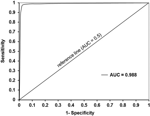
From these 16 structures the simulation of the data is performed, where the configuration (14-20-1) selected 14 inputs, 20 neurons and 1 output in the Scaled Conjugate Gradient (SCG) function with an assignment of weights described in Table 3. This configuration presents a mean-squared error (MSE) of 0.0028151, quadratic regression of 0.99%, Receiver Operating Characteristic (ROC) curve equal to 0.988 (Figure 9) and percentage of prediction on data not entered in the learning module of 92.86%. The simulation was performed with an array in the processing module of 1,000 iterations, a goal equal to zero and a maximum of 25 faults. The data obtained from the validation tests show results with high predictions. This corresponds to the selection of ANN structure with better performance in the learning tests, where 80 structures configurations with different parameters were performed.

Table 3. Assignment of weights inside the backpropagation structure and SGC function.

	Neurons
	1	2	3	4	5	6	7	8	9	10	11	12	13	14	15	16	17	18	19	20
Resistance	−0.420	0.313	−0.468	0.130	−0.536	−0.411	0.727	0.838	0.295	0.385	−0.441	0.128	−0.807	0.203	−0.893	−0.411	−0.032	0.738	−0.494	−0.420
Texture	0.510	0.007	0.423	0.229	−0.234	−0.749	0.125	0.127	0.900	0.240	−0.650	−0.477	0.092	0.662	0.806	0.657	−0.622	−0.734	0.066	0.117
Deposits	0.438	0.662	0.368	0.082	0.320	0.399	−0.114	0.460	0.884	0.210	0.238	0.162	0.142	0.163	−0.213	−0.630	0.653	0.438	0.641	−0.407
Fracture Density	0.301	−0.395	0.134	0.200	0.192	0.559	−0.703	−0.546	−0.357	−0.685	−0.385	0.150	−0.364	−0.260	0.439	0.365	0.717	−0.066	0.381	0.423
Morphogenesis	0.616	0.623	−0.599	0.733	0.188	0.365	0.095	−0.043	−0.076	−0.330	−0.350	0.531	−0.038	0.194	0.033	0.211	0.188	0.200	−0.296	0.648
Elevation	0.438	0.013	−0.421	−0.277	0.032	0.497	0.869	0.426	−0.312	−0.496	0.223	0.547	0.585	0.094	−0.022	0.387	−0.252	0.710	0.408	0.339
Aspect	0.573	0.383	0.063	−0.803	0.782	0.274	−0.070	−0.054	0.462	0.123	−0.354	−1.080	−0.662	−0.046	0.665	0.541	0.174	−0.366	−0.816	0.496
Curvature	0.186	0.382	0.090	−0.379	−0.919	0.015	0.355	0.196	0.641	−0.438	0.673	0.079	−0.321	−0.548	0.277	0.086	0.269	0.453	0.783	0.355
Distance Rivers	−0.462	−0.662	−0.520	0.400	0.051	−0.249	−0.633	0.227	−0.203	0.768	0.018	−0.325	0.246	0.319	0.380	−0.541	0.443	0.166	0.609	−0.622
Distance Roads	−0.363	−0.507	0.118	0.194	−0.388	0.296	0.108	0.763	0.487	−0.764	0.227	0.163	0.283	0.257	0.043	0.110	0.332	0.347	0.373	0.221
Slope	−0.182	−0.216	−0.759	−0.755	0.439	0.164	−0.104	0.516	0.175	−0.685	0.676	0.260	0.026	0.698	−0.055	−0.539	0.622	0.333	0.248	0.341
Rugosity	−0.518	−0.579	0.703	0.511	−0.436	−0.787	−0.358	−0.182	0.120	−0.224	−0.667	−0.632	−0.462	0.813	0.422	0.391	−0.700	0.499	0.242	−0.332
SPI	−0.604	−0.094	−0.227	−0.592	0.127	−0.122	−0.080	−0.312	0.458	0.145	0.047	−0.489	0.263	0.614	0.440	−0.477	−0.473	−0.401	0.122	−0.735
TWI	−0.681	0.387	−0.691	−0.261	0.433	0.662	0.464	0.623	−0.099	0.237	0.291	−0.155	−0.710	−0.628	−0.501	−0.565	0.397	0.087	−0.350	0.065

These processes were monitored so as not to generate an overlearning and overfitting in the ANN and in this way not to include an error in the estimation of the prediction to landslide. Also, this process takes into account two aspects related to the variables that were processed. First, the number of variables (14) was a fixed value, standardizing the learning tests within the ANN. Second, the number of variables entered ensured better results in the ANN simulation. From this information, the best structures (16) were selected to generate the simulation of the susceptibility to landslide of each of these structures. The simulation of the 16 structures takes into account the amount of landslides inventoried (50% for simulation), the other landslides (50% not entered) were used in the validation of the model created by ANN (Figure 8). With the processing of this structure and its simulation, the data are imported to ArcMap, which generates the graphical output (Cristina et al. 2016). The results show five classification ranges of susceptibility to landslides: very high, high, moderate, low and very low, calculated through the information simulated in the ANN, and describe the degree of instability with respect to slope movements (Figure 9), aspects that also take into account the parametric information that involves establishing a numerical range prioritizing the degree of affect of the activity of landslide in the terrain (Pradhan and Lee 2010; Pradhan et al. 2010).

Figure 8. Landslide taken for the neural network in the north zone (a), simulation of the ANN (b) and inventory of landslide (c).

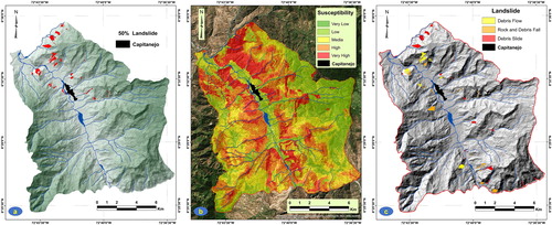
Figure 9. Susceptibility map for landslides.

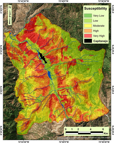
The very low and low susceptibility regions have a total area of 56.8 km² and occur in areas of low slope. Their distribution can be seen in the west, east and the margins of the Chicamocha River, and these regions are characterized as being associated with resistant rocks with low fracturing density. The region with moderate susceptibility presents an extension of 57.8 km² and is characterized by slopes of moderate to high slope with strong erosive and very discharged processes, where the structural aspects of the zone control the activity of rock erosion and erosion in the banks of the Chicamocha River. The region of high and very high susceptibility presents an extension of 91.6 km². These are areas with active slope movements (landslides) that appear on high slopes with high discharge, and are affected by the action of the drainage type (over slate) that in turn causes high fracturing density, a condition that affects the margins of the urban perimeter of the municipality of Capitanejo and the main roads.

The conditions exposed in the susceptibility model generated, show a close relationship with the activity recorded on the surfaces of the area evaluated, describing the effectiveness of the method in predicting regions with high potential for instability, important data, since the ANN model work only with 50% of the data of landslide events present, the rest of the landslide served as validators of the information generated by the ANN, where its prediction was 92.86%, a condition that presents a high confidence rate on the evaluation of these regions for purposes of attention by government plans for the municipality, as well as the information generated, exposes the quality of the processing of the ANN, to have a prediction a little higher than the works cited here. Another important point in the development of this method is the degree of detail generated by the cartographies incorporated in the methodology, the evaluation 365 based on a cartographic base of greater detail and scale of work, a better specialization and differentiation of geomorphological units and active processes, so this will result in greater efficiency and accuracy of results, improving the processing of the ANN, its possibilities and degree of certainty. Finally, the design of this type of mathematical simulation models to obtain areas with future events of instability due to landslide in a regional and local character within the national territory, have been little studied and their application within the management policies of The risk is only in its development phase, with studies such as this, support in the implementation of methodologies in the field of environmental management of the territory.

5. Discussion

The geological and geomorphological conditions of the study area evaluated for their ability to generate events of landslides and that are appropriate in each one of their variables do not maintain complete similarity for the creation of these events. Where the variables: resistance, texture, surface formations, fracture density, morphogenetic, elevation, aspect, curvature, distance to rivers, distance to roads, slope, rugosity, SPI and TWI that have been studied in the ANN modeling (Lee et al. 2003; Lee 2007; Pradhan and Lee 2010; Pradhan et al. 2010). Variables such as the elevation, rugosity and curvature are not directly related to the generation of landslide, and are conditions that may be affected by other aspects, such as the morphology of the region that develops steep slopes to steep related to the type of rock, being this is an interaction between sandstones, siltstones and conglomerates. In addition, these aspects generate slight changes in the relationship of each variable when they correlate with the stability of the rocks and soils present in the region, generating areas with high rates of surface erosion, gullies and furrows. The rugosity frames a parameter of instability in the surfaces with low coefficients or zones with a smooth slope–elevation relationship that, in turn, are within the geometries of flat curvature. This last variable also has a moderate incidence on concave geometries, these areas being more prone to mass movements. Other factors that influence the modification of the parameters of these variables and increase the instability conditions in rocks and soils are the structural and climatic aspects.

As a result of the morphological and morphometric characteristics of the terrain provided by the structural and climatic activity, variables such as elevation do not behave in accordance with description of landslide generation whereby a factor of instability is established with each ascending topographic level. This situation in the region of study shows processes of instability in rocks and soils between 1,231 m and 1,409 m, the range where the greatest number of landslides occurs. In addition, this parameter can be associated to strong slope changes (20°–40°) and rock type (shale). The variables of rugosity and curvature are other factors that are not related to the generation of landslides according to their description within the morphometric variables. Rugosity frames a parameter of instability in the surfaces with higher coefficients, and curvature is described in regions where the geometric surface of the slopes presents a concave form so that the movement takes place. These conditions for the study area have differences in rugosity which generate landslides on surfaces with low rugosity or flat zones, an aspect also associated to the curvature variable.

On the other hand, the distance to river variables SPI and TWI show a direct correlation with the landslide events. These regions describe a behaviour where the climate factor controls these events of instability, and in turn, control weathering and erosion processes in the margins of the river, a characteristic that is described as presenting a moderate to low rate of runoff. However, in an asymptotic form, the morphostructural configuration generates high rates of fracturing density and abrupt changes in the landscape, which magnify the erosive processes on the slopes. As a result of the interconnection of these events, a series of deposits of alluvial-type “dejection cones” are found in the topographically-low regions, this being a current contrast of present events in the region. In turn, the morphogenetic record exposes regions with alluvial fans of different orders, a condition that shows an eventuality of accumulation processes of material with accentuated erosive surfaces. In addition, the topography conditions frame strong erosive processes where hillside deposits develop ‘talus cones’.

These relationships between the variables and the generation of landslide allow to identify the conditions that present the highest incidence of instability on the slopes, being a new source of study for the identification and description of the causative factors on a more detailed scale. From the data generated it is observed that the exposed methodology allows to know the zones of greater susceptibility to landslide. These areas within environmental policies have a very high relevance, being necessary in the early stages of territorial planning. As well, this methodological approach is developed in areas of little extension or that is linked to work scales 1: 25,000 or 1: 50,000, being a tool of good prediction according to the variables entered in the learning module of ANN. In addition, it has the advantage that it is an effective and low-cost prevention tool. It also allows for a retroactive analysis to establish the sectors with anthropic activities indicating the degree of affection to the risks that can be generated in these regions.

6. Conclusions

Within the model proposed for obtaining susceptibility to landslide, it was established that there was instability on the surfaces of the banks of the Chicamocha river valley. Conditions that are related by lithology (shales), structural configuration, and slopes mark a continuous process of rock weathering. As a result of this, strong erosive states are generated which, together with the degree of fracturing of the rocks, form the main events of landslide in the study region. The events in the study region are presented as debris flows, followed by rotational and translational slides. Additionally, these conditions are compounded by climatic factors that accentuate the erosion events on the margins of the streams, producing large displacements of rocky material that is deposited in the margins of the Chicamocha River. The model simulated by the ANN was created under the parameters of the backpropagation algorithm in the SCG and presents an architecture (14-20-1) that simulates a regional configuration in terms of the susceptibility to landslides with great precision. This model presents a prediction of 92.86% of movements that were not entered in the learning module, which corresponds to 50% of the total landslides described in the region. In addition, the simulation of the neural network shows the AUC of the ROC curve with a specificity value against the sensitivity of the model equal to 0.988 (Figure 10).

Figure 10. ROC curve of the landslide susceptibility model obtained using an ANN.

Author contributions

For research articles, work presented in this paper is a collaborative development by all authors. Joaquin Valencia and Antonio Martínez-Graña processed the data in GIS. Joaquin Valencia and Antonio Martínez-Graña processed the geological and geomorphological context. The manuscript was written by all authors and revised-corrected by Antonio Martínez-Graña.

Disclosure Statement

The authors declare no conflicts of interest.

Additional information

Funding

This research was funded by projects from the Ministry of Economy and Competitiveness CGL2015-69919-R and CGL2015-67169-P.

References

- Akgun A. 2012. A comparison of landslide susceptibility maps produced by logistic regression, multi-criteria decision, and likelihood ratio methods: a case study at İzmir, Turkey. Landslides. 9:93–106.
- Akgun A, Kıncal C, Pradhan B. 2012a. Application of remote sensing data and GIS for landslide risk assessment as an environmental threat to Izmir city (west Turkey). Environ Monit Assess. 184:5453–5470.
- Akgun A, Sezer EA, Nefeslioglu HA, Gokceoglu C, Pradhan B. 2012b. An easy-to-use MATLAB program (MamLand) for the assessment of landslide susceptibility using a Mamdani fuzzy algorithm. Comput Geosci. 38:23–34.
- Alcantara-Ayala I. 2002. Geomorphology, natural hazards, vulnerability and prevention of natural disasters in developing countries. Geomorphology. 47:107–124.
- Aleotti P, Chowdhury R. 1999. Landslide hazard assessment: summary review and new perspectives. Bull Eng Geol Environ. 58:21–44.
- Anderson D, McNeill G. 1992. Artificial neural networks technology. Utica: Kaman Sciences Corporation.
- ASF. Dataset: ASF DAAC 2015, ALOS PALSAR_Radiometric_Terrain_Corrected_high_res. Includes Material © JAXA/METI 2007. doi:10.5067 / Z97HFCNKR6VA. (Accessed 2016 November 12).
- Ayala FJ. 1987. Introduction to Geological Risk. IGME (Instituto Geologico y Minero de España. ), Serie Geologıa Ambiental, Madrid; p. 3–19. (reference in Spanish)
- Ayala-Carcedo F, Cantos J. 2002. Natural risks. Barcelona, España: Ariel. (reference in Spanish)
- Ayalew L, Yamagishi H. 2005. The application of GIS-based logistic regression for landslide susceptibility mapping in the Kakuda- Yahiko Mountains, Central Japan. Geomorphology. 65:15–31.
- Bathrellos GD, Gaki-Papanastassiou K, Skilodimou HD, Papanastassiou D, Chousianitis KG. 2012. Potential suitability for urban planning and industry development by using natural hazard maps and geological – geomorphological parameters. Environ Earth Sci. 66: 537–548.
- Bathrellos GD, Skilodimou HD, Chousianitis K, Youssef AM, Pradhan B. 2017. Suitability estimation for urban development using multi-hazard assessment map. Sci Total Environ. 575:119–134.
- Bhardwaj A, Venkatachalam G. 2014. Landslide hazard evaluation using artificial neural networks and GIS. In Landslide science for a safer geoenvironment. Cham: Springer; p. 397–403.
- Boinet T, Bourgois J, Mendoza H. 1989. The Fault of Bucaramanga (Colombia), its function during the Andean Orogeny. Geol Norandina. 11:3–10. (Reference in Spanish).
- Botzen WJ, Aerts J, Van den Bergh J. 2013. Individual preferences for reducing flood risk to near zero through elevation. Mitig Adapt Strateg Global Change. 18:229–244.
- Campbell CJ. 1965. The Santa Marta wrench fault of Colombia and its regional setting. Fourth Caribbean Geological Conference. Trinidad. Memoir 247–261.
- Cardona OD, Hurtado JE, Duque G, Moreno A, Chardon AC, Velasquez LS, Prieto SD. 2004. Relative risk dimensioning and management: Methodology using indicators at the national level. BID/IDEA. Recovered on November 16, 2016: http://idea.unalmzl.edu.co/documentos/02%20Fundamentos%20Metodologicos%20Indicadores%20BID-IDEA%20Fase%20I.pdf.
- Carrara A, Cardinali M, Detti M, Guzzetti F, Pasqui V, Reichenbach P. 1991. GIS techniques and statistical models in evaluating landslide hazard. Earth Surf Process Landf. 16:427–445.
- Cediel F, Shaw RP, Caceres C. 2003. Tectonicassembly of the North Andean block. In: Bartolini C, Bufler RT, Blickwede J, editors. The Circum Gulf of Mexico and the Caribbean: Hydrocarbon Habitats, Basin Formations and Plate Tectonics. American Association of Petroleum Geologists, Memoirs 79:815–848.
- CEPAL. 2012. Valuation of damages and losses: winter wave in Colombia 2010-2011. Bogota.: Publicación de las Naciones Unidas. (reference in Spanish)
- Chacon J, Irigaray C, Fernandez T, EI, Hamdouni R. 2006. Engineering geology maps: landslides and geographical information systems. Bull Eng Geol Environ. 65:341–411.
- Cooper MA, Addinson FT, Alvarez R, Coral M, Graham RH, Hayward SH, Taborda A. 1995. Basin development and tectonic history of the Llanos Basin, Eastern Cordillera, and Middle Magdalena Valley, Colombia. Am Assoc Pet Geol Bull. 79: 1421–1443.
- Costa JE, Baker VR. 1981. Surficial geology. Building with the earth. New York: Wiley.
- Cristina B, Nieves L, Samuel A. 2016. Statistical and spatial analysis of landside susceptibility maps with different classification systems. Enviro Earth Sci. 75: 1318.
- Cruden DM. 1991. A Simple definition of a landslide. Bull Int Assoc Eng Geol. 43: 27–29.
- Cruden DM, Varnes DJ. 1996. Landslides: investigation and mitigation, Chapter 3 “Landslide types and processes”. Washington D.C.: National Academy Press, Transportation Research Board Special Report 247.
- De Brio B, Sanz A. 2007. Redes neuronales y sistemas borrosos. México DF, México: Alfaomega.
- Ercanoglu M, Gokceoglu C. 2002. Assessment of landslide susceptibility for a landslide-prone area (north of Yenice, NW Turkey) by fuzzy approach. Environ Geol. 41:720–730.
- ESRI.Environmental Systems Research Institute. [accessed 2017 January 1] Obtenido de http://desktop.arcgis.com/es/arcmap/latest/extensions/main/about-arcgis-for-desktop-extensions.htm
- Felicisimo AM. 1994. Digital terrain models. Oviedo: Pentalfa. Recovered on November 16, 2016, from http://www.etsimo.uniovi.es/∼feli. (reference in Spanish).
- Fell R, Corominas J, Bonnard C, Cascini L, Leroi E, Savage W. 2008. Guidelines for landslide susceptibility, hazard and risk zoning for land-use planning. Eng Geol. 102:85–98.
- Gallant JC, Hutchinson MF. 2008. Digital terrain analysis. In McKenzie N J, Grundy MJ, Webster R, Ringrose-Voase AJ, editors. Guidelines for surveying soil and land resources. Australian Soil and Land Survey Handbook Series (Vol. 2). Melbourne: CSIRO.
- Gardiner CW. 1985. Handbook of stochastic methods (Vol. 3). Berlin: Springer.
- Gokceoglu C, Aksoy H. 1996. Landslide susceptibility mapping of the slopes in the residual soils of the Mengen region (Turkey) by deterministic stability analyses and image processing techniques. Eng Geol. 44:147–161.
- Hoek E, Brown ET. 1997. Practical estimates of rock mass strength. Int J Rock Mech Mining Sci. 34:1165–1186. V
- IDEAM. Institute of Hydrology, Meteorology and Environmental Studies of Colombia. [accessed 2016 December 28] Obtenido de http://www.ideam.gov.co/ (reference in Spanish).
- INGEOMINAS 2002. National catalog of landslide. Instituto de Investigacion e Informacion Geocientifica. Bogota: Instituto de Investigacion e Informacion Geocientifica (reference in Spanish).
- Julivert M, Tellez N. 1961. Geology of the W slope of the Eastern Cordillera in the sector of Bucaramanaga. Boletin De Geologia, Universidad Industrial De Santander; p. 39–42. reference in Spanish).
- Lee S. 2007. Landslide susceptibility mapping using an artificial neural network in the Gangneung area, Korea. Int J Remote Sens. 28:4763–4783.
- Lee S, Park I, Choi JK. 2012. Spatial prediction of ground subsidence susceptibility using an artificial neural network. Environ Manag. 49:347–358.
- Lee S, Ryu JH, Lee MJ, Won JS. 2003. Use of an artificial neural network for analysis of the susceptibility to landslides at Boun, Korea. Environ Geol. 44:820–833.
- Lee S, Ryu JH, Won JS, Park HJ. 2004. Determination and application of the weights for landslide susceptibility mapping using an artificial neural network. Eng Geol. 71:289–302.
- Leon LA. 1991. Geological map of the Department of Santander. Scale 1: 800.000. Boletín de Geología, Universidad Industrial de Santander; p. 53–63 (reference in Spanish).
- Martinez-Graña AM, Goy JL, Zazo C. 2016. Geomorphological applications for susceptibility mapping of landslides in natural parks. Environ Eng Manag J. 15:327.
- Martinez-Graña AM, Goy JL, De Bustamante I, Zazo C. 2014. Characterisation of environmental impact on resources, using strategic assessment of environmental impact and management of natural spaces of “Las Batuecas-Sierra de Francia” and “Quilamas” (Salamanca, Spain). Environ Earth Sci. 71:39–51.
- Martinez-Graña AM, Goy JL, Zazo C, Yenes M. 2013. Engineering geology maps for planning and management of natural parks: “Las Batuecas-Sierra de Francia” and “Quilamas” (Central Spanish System, Salamanca, Spain). Geosciences. 3:46–62.
- Matich DJ. 2001. Informática Aplicada a la Ingeniería de Procesos – Orientación I. En D. J. Matich, Neural Networks: Basic concepts and applications. Argentina: Universidad Tecnológica Nacional; p. 55 (reference in Spanish).
- Matula M. 1981. Rock and soil description and classification for engineering geological mapping report by the IAEG Commission on Engineering Geological Mapping. Netherlands: Bulletin of Engineering Geology and the Environment.
- Nefeslioglu HA, Sezer E, Gokceoglu C, Bozkir AS, Duman TY. 2010. Assessment of landslide susceptibility by decision trees in the metropolitan area of Istanbul, Turkey. Math Probl Eng. 2010:1–15.
- Ohlmacher GC. 2000. The relationship between geology and landslide hazards of Atchison, Kansas, and vicinity. Kansas: Kansas Geological Survey.
- Olaya V. 2009. Basic land-surface parameters. In: Hengl T, Reuter HI, editors. Geomorphometry: concepts, software, applications. Developments in Soil Science 33. Amsterdam: Elsevier; p. 141–169.
- Pike RJ. 1995. Geomorphometry: progress, pratice, and prospect. Z Geomorphol. 101:221–238.
- Pistocchi A, Luzi L, Napolitano P. 2002. The use of predictive modeling techniques for optimal exploitation of spatial databases: a case study in landslide hazard mapping with expert system-like methods. Environ Geol. 41:765.
- Poudyal CP, Chang C, Oh HJ, Lee S. 2010. Landslide susceptibility maps comparing frequency ratio and artificial neural networks: a case study from the Nepal Himalaya. Environ Earth Sci. 61:1049–1064.
- Pradhan B, Lee S. 2010. Landslide susceptibility assessment and factor effect analysis: backpropagation artificial neural networks and their comparison with frequency ratio and bivariate logistic regression modelling. Environ Modell Softw. 25:747–759.
- Pradhan B, Lee S, Buchroithner MF. 2010. A GIS-based back-propagation neural network model and its cross-application and validation for landslide susceptibility analyses. Comput Environ Urban Syst. 34:216–235.
- Regmi AD, Devkota KC, Yoshida K, Pradhan B, Pourghasemi HR, Kumamoto T, Akgun A. 2014. Application of frequency ratio, statistical index, and weights-of-evidence models and their comparison in landslide susceptibility mapping in Central Nepal Himalaya. Arab J Geosci. 7:725–742.
- Saha AK, Gupta RP, Sarkar I, Arora MK, Csaplovics E. 2005. An approach for GIS-based statistical landslide susceptibility zonation— with a case study in the Himalayas. Landslides. 2:61–69.
- SIMMA. National System of Landslide “SGC”. [Accessed 2017 January 3] Obtenido de http://simma.sgc.gov.co/#/public/basic/ (reference in Spanish).
- Simpson PK. 1990. Artificial neural system—foundation, paradigm, application and implementation. New York: Pergamon Press.
- Soeters R, Van Westen CJ. 1996. Slope instability recognition, analysis and zonation. Washington, D.C.: National Academy Press.
- Suarez J. 2009. Slides: geotechnical analysis (Vol. I). Bucaramanga: Universidad Industrial de Santander. (reference in Spanish).
- Toro J. 1990. The termination of the Bucaramanga Fault in the Cordillera Oriental, Colombia, Master’s Thesis. Tucson: University of Arizona, Department of Geosciences.
- UNESCO. 1976. Engineering geological mapping. A guide to their preparation. Prepared by the Commission on Engineering Geological Maps of the International Association of Engineering Geology. Paris: Unesco Press.
- Valencia MA, Yañes C, Sanchez LP. 2006. Algoritmo Backpropagation para Redes Neuronales: conceptos y aplicaciones. Mexico: Instituto Politécnico Nacional Centro de Investigación en Computación.
- Van der Hammen T. 1958. Stratigraphy of Tertiary and Maestrichtian Continental and tectogenesis of the Colombian Andes. Boletín Geológico. Ingeominas Bogotá. 6:67–128. (reference in Spanish).
- Vargas RH, Arias AT, Jaramillo LC, Tellez NL. 1976. Geology of the plates 136 malaga and 152 soata, quadrangulo i-13, explanatory memory. instituto colombiano de geología y minería, ingeominas 80–93. (reference in Spanish).
- Yalcin A, Reis S, Aydinoglu A, Yomralioglu T. 2011. A GIS-based comparative study of frequency ratio, analytical hierarchy process, bivariate statistics and logistics regression methods for landslide susceptibility mapping in Trabzon, NE Turkey. Catena. 85:274–287.