Multi-sensor observation fusion scheme based on 3D variational assimilation for landslide monitoring

Abstract

Multi-sensor observation is very important for monitoring landslide disasters. Since various surveying techniques are currently available for detecting variational slope activities from different perspectives, studies have focused on integration of multi-source information for the analysing landslide displacements. In this study, a general multi-source data fusion scheme for landslide monitoring based on three-dimensional variation (3DVar) data assimilation was developed. The scheme was used to fuse different observations of Xishancun Landslide in Li County, Sichuan Province, China. First, the displacement observations obtained by a Global Positioning System (GPS) and Borehole Inclinometers (BIs) were assimilated for accurate evaluation of slope activities. Then, slope Stability Index (SI) was introduced to validate the assimilation results within a time interval. SI_Assi values calculated using the integration model developed in the present study were compared with SI_FS simulated by a physically based landslide model. The correlation coefficient between them ss 0.75, which is larger than those with SI_GPS (0.45) or SI_BIs (0.41) values determined by the GPS and BIs respectively. The assimilation results are thus confirmed to be more credible for slope stability simulation.

Keywords:

• Landslide monitoring
• 3DVar assimilation
• multi-sensor
• observation
• slope stability

1. Introduction

A landslide is a hazardous geological phenomenon that frequently occurs globally (Schuster 1996; Pradhan and Buchroithner 2012). Landslides pose a threat to millions of lives and diverse structures and infrastructure such as buildings, roads, and reservoirs (Pourghasemi et al. 2012; Lu et al. 2015). They sometimes occur on a very large scale, resulting in heavy casualties and economic losses. As a landslide-prone country, China currently contends with the threat of great landslides, especially in the south-western mountainous region (Li et al. 2016a; Li et al. 2017). It has been reported that there are presently more than 90,000 potential landslides threating about 70 cities and villages of China with at least 10% of the residents in direct danger (Zhou et al. 2005; Huang and Li 2011; Liu et al. 2013; Li et al. 2016b). It is very important to construct the systematic platform for monitoring landslide processes and identifying landslide characteristics.

A variety of monitoring techniques for slope failure survey have been developed and used for landslide monitoring in recent years (Gili et al. 2000; Travelletti et al. 2012; Zhao et al. 2018). Among them, remote sensing techniques such as those that utilize a synthetic aperture radar (SAR)（Liu et al. 2013) and very high resolution (VHR) satellite images (Debella-Gilo and Kääb 2011) are used to monitor regional slope deformation. However, their low temporal resolution, which is due to the long revisit cycle of the utilized satellite systems, may result in the inability to capture slope failure variations (Greif and Vlcko 2012). Nevertheless, some in situ devices are particularly known for their high-temporal and continuous sequential observations. For example, the Global Positioning System (GPS) has been increasingly employed in the study of landslide surface movements (Gili et al. 2000; Wang 2011; Huang et al. 2017), but its accuracy is affected by some inherent errors such as clock bias, ionosphere error, and troposphere error (Parkinson 1996). Underground inclinometers are used to determine internal slope changes (Chang et al. 2005; Segalini and Carini 2013) but the used inclinometers to calculate the surface displacement may also cause some uncertainties. These devices are thus limitedly effective for slope failure survey through direct monitoring. Accordingly, multi-sensor networks have been developed for gathering diverse information from underground layers and determining the topographic characteristics of the slope surface and the meteorological conditions (Qiao et al. 2013). Multi-source data can be used to enhance the effectiveness of sensors and achieve better research analyses from different perspectives (Lee and Pradhan 2007; Dewitte et al. 2008; Corsini et al. 2013; Bardi et al. 2016). Landslide monitoring using multi-source data particularly facilitates the illustration of the underlying cause of the slope activities (Du et al. 2013; Xia et al. 2013; Jiang et al. 2016). However, multi-source data may also contain significant discrepancies regarded to data scale, resolution, format, and other factors, and it may complicate the data processing. Moreover, observation errors and uncertainties negatively affect the accuracies of the results, leading to a biased estimation of the slope stability (Liao et al. 2012).

In this study, we developed a multi-sensor observation fusion scheme based on three-dimensional variational (3DVar) assimilation to fuse two types of data, namely, GPS and Borehole Inclinometers (BIs) data. First, 3DVar assimilation method is mathematically premised on optimal state estimation, in which historical data is used to reduce analysis error under constraints of dynamic consistency to infer present state through best solutions (Dee and Da Silva 1998; Renzullo et al. 2008). This method was first applied in the fields of meteorology and oceanography (Charney et al. 1969; Thompson 1969). So far, variational assimilation has been implemented and investigated in numerous studies such as those on weather prediction (Barker et al. 2004), wind field modelling (Ulazia et al. 2016), land surface temperature inversion (Carrera et al. 2016), and remote sensing of soil moisture (Mechri et al. 2016). On the other hand, there are kinds of errors and inherited weaknesses in landslide observations, which may bring disadvantages to slope stability estimation. For example, random errors in BIs could be smaller than 1mm but the their measurement magnitude is as much as a few centimetres per 30 m deep (Stark and Choi 2008); on the contrary, GPS affords millimetre-accurate landslide movement observations (Wang 2013), but the rough results contain more random noises in related to ionospheric and tropospheric influences (Huang et al. 2016).

The rest of this paper is organized as follows. Section 2 firstly presents the general framework to fuse multi-source observations based on 3DVar assimilation method. Section 3 introduces study area and relevant data including GPS and BIs data. Results are discussed and summarized in Section 4 and Section 5, respectively.

2. Observation fusion method

2.1. General framework

Figure 1 illustrates the multi-sensor observation fusion scheme developed in the present study. Considering the errors of historical multi-sensor data, the cost functions derived from the parameters are implemented to generate the assimilated data, which contains corrections for the current epoch based on the modelled error information and real-time information.

Figure 1. Framework of the proposed multi-sensor observation fusion scheme.

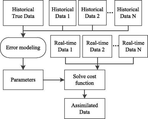
2.2. Assumption and error modelling

It is assumed that the error (ε) values of the multi-sensor observation at a location (x, y) in a long time series are normally distributed with the density function f (ε | μ, σ), where μ is the expectation, and σ is the square root of the variance. As expressed by Equation (1)(1) $$f\left(\epsilon |\mu ,\sigma \right)=\frac{1}{\sqrt{2\pi }\sigma }\text{exp}[-\frac{{(\epsilon -\mu )}^2}{2{\sigma }^2}]$$(1) , ε is mutually independent. These parameters are modelled using a monotonic (e.g. linear/non-linear or smooth) link function, and the error distribution can be subsequently determined.

(1) $$f\left(\epsilon |\mu ,\sigma \right)=\frac{1}{\sqrt{2\pi }\sigma }\text{exp}[-\frac{{(\epsilon -\mu )}^2}{2{\sigma }^2}]$$(1)

2.3. Cost function obtained by 3DVar assimilation

3DVar is a classic data assimilation method that involves the minimization of a prescribed cost function (Ide et al. 1997). It provides an optimal solution by considering the fields of the background and observation data. Based on 3DVar assimilation and the modelled parameters (μ, σ), the cost function can be formulated as follows: (2) $$J\left(X\right)=\frac{{\sum _{i=1}^N(Z_i-X_i)}^2}{\sum _{i=1}^N\left(\frac{1}{{\sigma }_i}\right)}$$(2)

where X denotes the location of the desired data, and Z_i is the ith kind of observation.

In the case of two input data series, the 3DVar cost function can be formulated as follows:

(3) $$\left\{\begin{array}{c}J\left(X\right)=J_b+J_o\\ J_b\left(X\right)=\frac{1}{2}{\left(X-X^b\right)}^T{B}^{-1}(X-X^b)\\ J_o\left(X\right)=\frac{1}{2}{\left(H\left(X\right)-Y^O\right)}^T{R}^{-1}(H\left(X\right)-Y^o)\end{array}\right.$$(3)

where J_b is the cost function value for the analysis data (X^a) and background data (X^b), and J_o is the value for the analysis data and observation data (Y^o) in Figure 2. The matrixes B and R respectively represent the error variances of X^b and Y^o, and H is the linear projection function of Y^o into the dimensional space of X^b. H is an identity matrix when X^b and Y^o are in the same dimensional space.

Figure 2. Results of 3DVar assimilation.

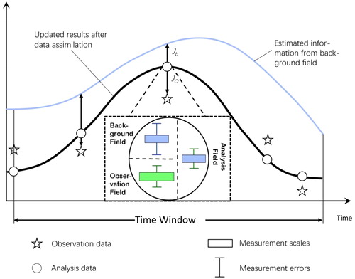
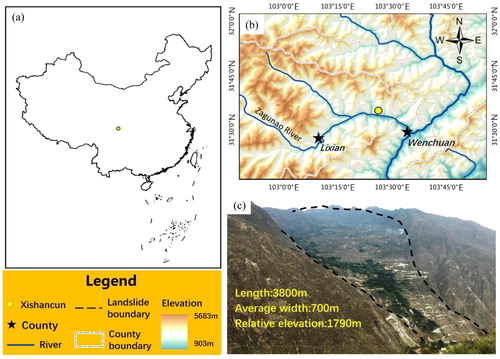
Figure 3. Study area: (a) map of China; (b) location of ‘Xishancun Landslide’; (c) view of ‘Xishancun Landslide’.

To seek for the solution (analysis values X^a) of the assimilation problem in Equation (3)(3) $$\left\{\begin{array}{c}J\left(X\right)=J_b+J_o\\ J_b\left(X\right)=\frac{1}{2}{\left(X-X^b\right)}^T{B}^{-1}(X-X^b)\\ J_o\left(X\right)=\frac{1}{2}{\left(H\left(X\right)-Y^O\right)}^T{R}^{-1}(H\left(X\right)-Y^o)\end{array}\right.$$(3) , the differential Equation (4)(4) $$\left\{\begin{array}{c}{X}^a=\mathit{\text{argmin}}\left(J\left(X\right)\right),X\in R\\ \nabla J\left(X\right)=B^{-1}\left(X-X^b\right)+H^T{R}^{-1}[H\left(X\right)-Y^o]\end{array}\right.$$(4) is used to minimize the cost function. Equation (5)(5) $$\left\{\begin{array}{c}\nabla J\left(\Delta X\right)=0\\ \Delta X={(B^{-1}+H^T{R}^{-1}H)}^{-1}{H}^T{R}^{-1}D\\ D=Y^o-H\left(X^b\right); X^a=X^b+\Delta X\end{array}\right.$$(5) expresses the iterative method for solving the problem. (4) $$\left\{\begin{array}{c}{X}^a=\mathit{\text{argmin}}\left(J\left(X\right)\right),X\in R\\ \nabla J\left(X\right)=B^{-1}\left(X-X^b\right)+H^T{R}^{-1}[H\left(X\right)-Y^o]\end{array}\right.$$(4)

(5) $$\left\{\begin{array}{c}\nabla J\left(\Delta X\right)=0\\ \Delta X={(B^{-1}+H^T{R}^{-1}H)}^{-1}{H}^T{R}^{-1}D\\ D=Y^o-H\left(X^b\right); X^a=X^b+\Delta X\end{array}\right.$$(5)

3. Study area and materials

3.1. Description of experimental area

The study area of the present work is located in South-western China, east of the Tibetan Plateau (Figure 3). It is 22 km from Wenchuan City, and is one of the most prone to severe geo-hazard areas, after being exposed to the 5.12 Wenchuan Earthquake in 2008 (Cui et al. 2011; Dai et al. 2011). The specifically considered ‘Xishancun Landslide’ located north of the Zagunao River is a large soil accumulation with a relative elevation of about 1790 m, slope length of about 3800 m, and average width of approximately 700 m (Xu et al. 2016).

3.2. Ground observation data

3.2.1. Equipment installation and data calibration

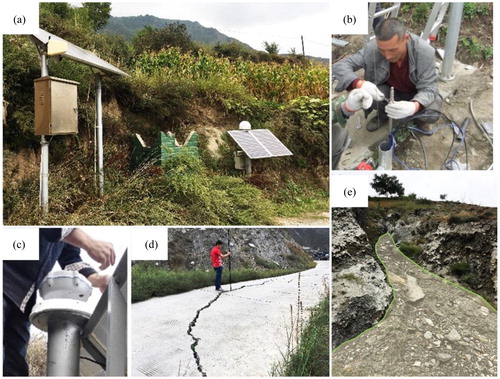
To detect the real-time slope displacement, three types of monitoring devices were installed on the slope surface (Figure 4), namely, a Global Positioning System, Borehole Inclinometers (BIs), and two rain gauges (RG). Some local instabilities such as positive and negative road subsidence and surface debris could occur in the neighbour of these sensors. All the devices are powered by solar energy so that they continuously work in 24-h 1 day. The data obtained by all the sensors is transmitted to a data centre through a General Packet Radio Service (GPRS).

Figure 4. Installation of the BIs and GPS on ‘Xishancun Landslide’: (a) Overview of sensors; (b) BIs installation; (c) GPS installation; (d) road subsidence found in study area; and (e) historical debris area in study area.

Table 1 gives the details of the three types of employed monitoring devices. The BIs and RG have the same data collection interval of 10 min, while the corresponding interval for the GPS is 2 h. Due to minimal data loss during the GPRS data transmission, the numbers of available data records were 2,560 for the GPS, 24,883 for the BIs, and 25,104 for the each RG. The duration time of the data acquisition is from January 1st, 2016 to November 17th, 2016.

Table 1. Details of data from GPS, BIs, and RG.

	GPS	BIs	RG
Duration of use	1/1/2016–11/17/2016
Data collection interval	2 h	10 min	10 min
Device type	Huace GPS Receiver X300 m	MEMS Fixed Inclinometer BGK 6150	Tipping Bucket Rain Collector QS-1501
Installation location	Surface	Underground	Surface
No. of data units	2,560	24,883	25,104
Accuracy	Horizontal: 2.5 mm +1 ppm Vertical: 5 mm +1 ppm	±10 arc s	±0.2 mm

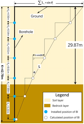
After difference calibration, the horizontal and vertical accuracies of the GPS data are respectively 2.5 mm ±1 ppm and 5 mm ±1ppm. BIs comprised six inclinometers connected by an aluminium alloy tube, with the one located deepest underground being at a depth of 42.78 m (Figure 5). Although BIs may not directly measure the horizontal movements of the casing (Stark and Choi, 2008), the tilt angle could be converted into horizontal displacement, as illustrated in Figure 5. The following equation is used.

(6) $$S=\sum L_i\text{sin}{\theta }_i$$(6)

where L_i is the distance between two neighbouring BIs. Because the tilt angle θ_i is rather small for each movement, L_i is considered to be close to the initially set pitch (K in Figure 5). Equation (6)(6) $$S=\sum L_i\text{sin}{\theta }_i$$(6) could be used to determine the incremental displacement at each inclinometer and the cumulative horizontal displacement.

Figure 5. BIs installation and displacement measurement.

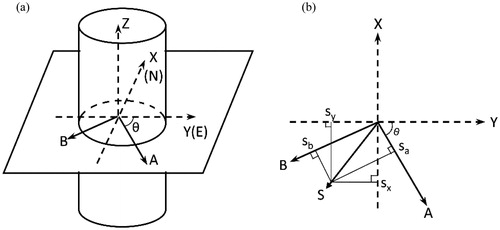
Figure 6 shows the coordinate calibrations of the BIs and GPS. The northward and eastward coordinates of the GPS are respectively denoted by X and Y, while the coordinates of the BIs in the horizontal plane are denoted by A and B (Figure 6(a)). There is a rotation angle θ between the two coordinate systems in Figure 6(b). The resultant horizontal displacement is calculated using Equation (7)(7) $$\left\{\begin{array}{c}{S}_{\text{GPS}}=\sqrt{{S_x}^2+{S_y}^2}\\ S_{\text{BIs}}=\sqrt{{S_a}^2+{S_b}^2}\end{array}\right.$$(7) .

(7) $$\left\{\begin{array}{c}{S}_{\text{GPS}}=\sqrt{{S_x}^2+{S_y}^2}\\ S_{\text{BIs}}=\sqrt{{S_a}^2+{S_b}^2}\end{array}\right.$$(7)

Figure 6 Calculation system for the standard BIs measurements.

3.2.2. Possible displacement based on GPS and BIs error estimation

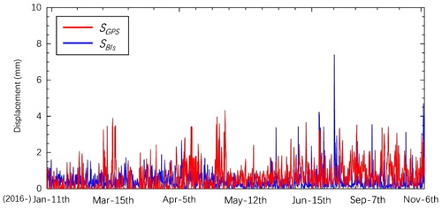
The variations of the slope surface displacements determined by the GPS and BIs after space and time calibration are shown in Figure 7. GPS has been proven enable millimetre-accurate recording of slope failure, but more random errors, introduced during signal transmission and by interferences, which still need to be carefully mitigated to achieve millimetre accuracy (Wang 2013). The process of it could be complicated sometimes in related to factors of ionospheric and tropospheric influences (Huang et al. 2016). Conversely, while BIs only afford measurement magnitudes, being as much as a few centimetres per 30 m (Stark and Choi 2008), their associated random errors, as in situ instruments, are smaller. Therefore, considering insufficient mitigation of random errors, the secondary errors from GPS are larger than from BIs.

Figure 7 Variations of the slope surface displacements determined by the GPS and Bis.

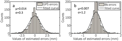
To verify the assumptions mentioned in Section 2.2, that the random errors of the GPS and BIs observations are normally distributed, the moving average (MA) method was used to fit the ‘true’ data for a 24 h duration. The obtained errors distributions for the GPS and BIs are shown in Figure 8. As can be observed, the errors for the two types of equipment range within −5 to 5 mm and −2 to 2 mm, respectively.

Figure 8 Error distributions for the (a) GPS and (b) BIs as obtained by the moving average method.

4. Results and discussion

4.1. Assimilation results for GPS and BIs

Based on the above analysis of the probable error distribution, two monitoring data were input to a 3DVar assimilation model, with the background (observation) field input being the data obtained by the GPS (or BIs). Figure 9 shows the cumulative slope surface displacements obtained by the GPS, BIs, and assimilation results. As can be observed, the sequence of the assimilation results is much closer to that of the GPS sequence at the 20th iteration step. With continuous assimilation, it subsequently becomes closer to the BIs sequence. In addition, the noise in the assimilation results gradually attenuates with increasing number of iterations.

Figure 9 3DVar results with increasing number of iterations.

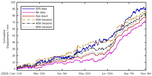
Figure 10 Convergence of the cost function with increasing number of iterations.

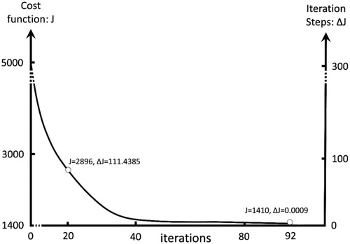
With increasing number of iterations, the derived cost function J finally coverages to 1410.2147 from the initial value of 4906.4473 (Figure 10). Considering that a threshold of 0.001 selected as the terminal iteration signal, the final iteration step (the 92nd iteration) degrades to 0.0009 from 111.4385 at the 20th iteration.

4.2. Analysis of slope stability

4.2.1. Determination of slope stability from displacements

Differing variation of the slope displacement affects the slope stability, which determines the occurrence of a landslide. Researchers have used different models to establish the relationship between the displacement and the slope stability (Al-Homoud and Tahtamoni 2000; McCombie 2009; Akbarimehr et al. 2013). Among them, the Unload-Load Displacement Response Ratio (ULDRR) model (Keqiang et al. 2017) emphasizes on the rainfall-induced micro-deformations of the slope in the simulation of the slope stability as follows. (8) $$\eta =\frac{{\gamma }_{-}}{{\gamma }_{+}}=\underset{\Delta L\to 0}{\lim }\left(\frac{\Delta R_{-}}{\Delta L_{-}}\right)/\left(\frac{\Delta R_{+}}{\Delta L_{+}}\right)$$(8)

where ΔL₊ (or ΔL₋) is the load (or unload) increment, ΔR₊ (or ΔR₋) is the load (or unload) response increment. In our test, the rainfall intensity is regarded as the load (L) acting on the slope system, and the induced displacement as the response (R) to the load.

In addition, γ₊ (or γ₋) is defined as the rainfall-induced deformation rate due to the load (or unload). In the elastic-plastic slope deformation state, the rate of the deformation response to the load (γ₊), is mostly equal to that of the unload (γ₋). However, the deference between γ₊ and γ₋ increases with increasing load. If the slope system is continuously loaded to destabilization, the load deformation ratio would tend to infinity (γ₊ → ∞) while γ₋ would remain constant. Under this condition, a very small load could induce a very large displacement response, and η would be close to 0. The slope is thus unstable when η is close to 0. In the present study, η is normalized as the stability index (SI) with a value range of 0–1. (9) $${SI}_{\eta }=\frac{{\eta }_i}{\text{max}(\eta )}$$(9)

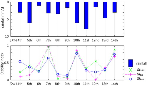
Figure 11 shows the variations of the daily rainfall and SI between October 4th and 14th, 2016. As can be observed, the daily rainfall is maximum at 7.8 mm/day on October 11th, and minimum at 1.0 mm/day on October 6th. In addition, more unstable processes may occur after heavier rainfall, such as on October 6th and 12th. Variations of SI extracted by three kinds of data indicate different changes in the test time window. BIs show that the highest unstable process occurs at the 12th. Moreover, SI_BIs exhibits more days (5 days) to be lower than SI_GPS and SI_Assi.

Figure 11 Rainfall and slope stability based on the ULDRR model.

4.2.2. Test of assimilation results based on slope mechanism

The slope stability determined by different methods may differ, resulting in errors in the monitoring of the slope failure. In further investigation, an attempt is made to incorporate the mechanism of the slope stability into the analysis to verify the present assimilation results.

A physical model referred as the Slope-Infiltration-Distributed Equilibrium (SLIDE) model is used to model the slope stability. SLIDE is a shallow rainfall-induced landslide model. Based on the rainfall infiltrating process, it simplifies the saturated-unsaturated seepage equation (Richards 1931) and integrates the contribution of the apparent cohesion to the shear strength of the soil and water level when the surface of the soil attains saturation (Liao et al. 2012; He et al. 2016). The detailed theory is available in the work of Liao et al. (2012). The model simulates the variations of the slope factor of safety (FS) in Equation (10)(10) $$\mathrm{F}\mathrm{S}\left(Z_t,t_i\right)=\frac{c+c\left(t\right)}{r_s{Z}_t\text{sin}\alpha \text{cos}\alpha }+\frac{\text{tan}\phi }{\text{tan}\alpha }$$(10) . The value of the SI_FS can be calculated using Equation (11)(11) $${SI}_{FS}=1-\frac{1}{{FS}_i}$$(11) . (10) $$\mathrm{F}\mathrm{S}\left(Z_t,t_i\right)=\frac{c+c\left(t\right)}{r_s{Z}_t\text{sin}\alpha \text{cos}\alpha }+\frac{\text{tan}\phi }{\text{tan}\alpha }$$(10)

(11) $${SI}_{FS}=1-\frac{1}{{FS}_i}$$(11)

The SLIDE model has been previously used to simulate rainfall-induced shallow landslides in Li County, where the Xishancun Landslide is located (Li et al. 2017). Therefore, soil parameters in the previous work were adopted in the present study to determine the variables in Equation (10)(10) $$\mathrm{F}\mathrm{S}\left(Z_t,t_i\right)=\frac{c+c\left(t\right)}{r_s{Z}_t\text{sin}\alpha \text{cos}\alpha }+\frac{\text{tan}\phi }{\text{tan}\alpha }$$(10) .

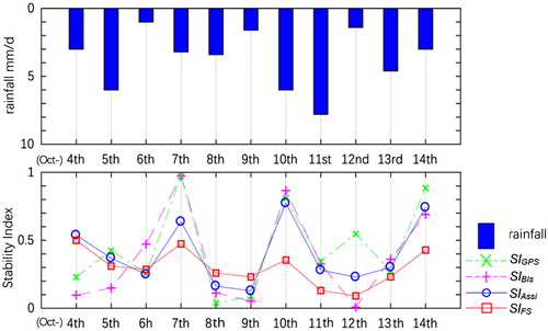
As can be observed from Figure 12, the variation of SI_FS over the entire test duration is closer to SI_Assi than those of SI_GPS and SI_BIs even when those are divergent for example on 7th and 12th. Further, the assimilation results regarding to slope failure are more accurate in SI_Assi than in SI_GPS and SI_BIs. For example, SI_GPS is 0.03 on 8th and SI_BIs is 0.01 on 12th, this kind of low values generally indicated a slop failure but it did not happen actually. Therefore, based on the analysis above, the assimilation results are thus confirmed to be more credible for slope stability simulation, by integrating the advantages afforded by the use of both GPS and BIs.

Figure 12 Comparisons of landslide stability index based on SLIDE and ULDRR models determined by GPS, BIs, Assi and FS results.

Furthermore, we have compared the assimilated results with the traditional fusion method-polynomial method (PM). In the fitted PM, the data from GPS and BIs is considered as sample data during 4th–10th, and other data during 11th–14th as tested data. Meanwhile, SI_PM from each tested data have been estimated by PM. As shown in Table. 2, the assimilated results (SI_Assi = 0.28, 0.23, 0.30, and 0.74) perform better than the results from PM in each estimated four days (SI_PM = 0.49, 0.36, 0.39, and 0.39), and are closer to the results from SLIDE model (SI_FS).

Table 2. Comparisons of Stability Index (SI) estimated from Assi, PM and SLIDE model.

Date (Oct.-)	SIAssi	SIPM	SIFS
11th	0.28	0.49	0.13
12th	0.23	0.36	0.09
13th	0.30	0.39	0.23
14th	0.74	0.39	0.43

5. Summary and conclusion

Multi-source observation is an advanced scientific method for monitoring landslides (Herrera et al. 2017). However, it faces challenge of the need to fuse multiple heterogeneous observation data for processing (Gravina et al. 2017). In the present study, a multi-sensor observation fusion scheme based on 3DVar assimilation is developed for the fusion of GPS and BIs data. Some major conclusions of this study can be summarized as follows:

1. Observations of the two considered sensors may differ for serial slope displacements, due to internal and external factors such as systematic data errors, noise, and data frequency. After estimating the observation errors, the cost function is constructed initially and iteration steps of it converge to less than 0.001 mm through the proposed multi-sensor observation fusion scheme

2. The results show that the proposed scheme based on 3DVar stands out in fusing multiple heterogeneous data. The utilized assimilation process particularly enables more accurate monitoring of slope failure. During a typical period with continuous rainfall, the slope stability extracted from the assimilation results (SI_Assi) was observed to be closer to that determined by simulation using a physical model than those observed by GPS (SI_GPS) and BIs (SI_BIs), respectively.

In further study, we will attempt to use the proposed scheme to fuse additional remotely sensed data such as those obtained by Interferometry Synthetic Radar (In-SAR) and Light Detection and Ranging (LiDAR). This is expected to enrich the acquired data to achieve spatial-temporal assimilation (Hunt et al. 2007).

Disclosure statement

No potential conflict of interest was reported by the authors.

Additional information

Funding

This work was supported by the National Basic Research Program of China (Grant No. 2013CB733204), National Natural Science Foundation of China (Grant No. 41501458), and China Postdoctoral Science Foundation Funded Project (Grant No. 2016M592860).

References

- Akbarimehr M, Motagh M, Haghshenas-Haghighi M. 2013. Slope stability assessment of the Sarcheshmeh Landslide, Northeast Iran, Investigated using InSAR and GPS observations. Remote Sens. 5(8):3681–3700.
- Al-Homoud AS, Tahtamoni WW. 2000. Reliability analysis of three-dimensional dynamic slope stability and earthquake-induced permanent displacement. Soil Dyn Earthquake Eng. 19(2):91–114.
- Bardi F, Raspini F, Ciampalini A, Kristensen L, Rouyet L, Lauknes TR, Frauenfelder R, Casagli N. 2016. Space-borne and ground-based InSAR data integration: the Åknes test site. Remote Sens. 8(3):237.
- Barker DM, Huang W, Guo YR, Bourgeois AJ, Xiao QN. 2004. A three-dimensional variational data assimilation system for MM5: implementation and initial results. Mon Weather Rev. 132(4):897–914.
- Carrera M, Bilodeau B, Russell A, Wang X, Belair S. 2016. Towards the implementation of L-band Soil Moisture Brightness Temperatures in the Canadian Land Data Assimilation System (CaLDAS). EGU Gen Assembly Conf Abstracts. 18:7520.
- Chang M, Chiu Y, Lin S, Ke TC. 2005. Preliminary study on the 2003 slope failure in Woo-wan-chai area, Mt. Ali Road, Taiwan. Eng Geol. 80(1):93–114.
- Charney JG, Halem M, Jastrow R. 1969. Use of incomplete historical data to infer the present state of the atmosphere. J Atmos Sci. 26(5):1160–1163.
- Corsini A, Castagnetti C, Bertacchini E, Rivola R, Ronchetti F, Capra A. 2013. Integrating airborne and multi-temporal long-range terrestrial laser scanning with total station measurements for mapping and monitoring a compound slow moving rock slide. Earth Surf Process Landforms. 38(11):1330–1338.
- Cui P, Chen XQ, Zhu YY, Su FH, Wei FQ, Han YS, Liu HJ, Zhuang JQ. 2011. The Wenchuan earthquake (May 12, 2008), Sichuan province, China, and resulting geohazards. Nat Hazards. 56(1):19–36.
- Dai FC, Xu C, Yao X, Xu L, Tu XB, Gong QM. 2011. Spatial distribution of landslides triggered by the 2008 Ms 8.0 Wenchuan earthquake, China. J Asian Earth Sci. 40(4):883–895.
- Debella-Gilo M, Kääb A. 2011. Sub-pixel precision image matching for measuring surface displacements on mass movements using normalized crosscorrelation. Remote Sens Environ. 115(1):130–142.
- Dee DP, Da Silva AM. 1998. Data assimilation in the presence of forecast bias. Quat J R Meteorol Soc. 124(545):269–295.
- Dewitte O, Jasselette JC, Cornet Y, Van Den Eeckhaut M, Collignon A, Poesen J, Demoulin A. 2008. Tracking landslide displacements by multi-temporal DTMs: A combined aerial stere-ophotogrammetric and LIDAR approach in western Belgium. Eng Geol. 99(1):11–22.
- Du J, Yin K, Lacasse S. 2013. Displacement prediction in colluvial landslides, Three Gorges Reservoir, China. Landslides. 10(2):203–218.
- Gili JA, Corominas J, Rius J. 2000. Using Global Positioning Sys-tem techniques in landslide monitoring. Eng Geol. 55(3):167–192.
- Gravina R, Alinia P, Ghasemzadeh H, Fortino G. 2017. Multi-sensor fusion in body sensor networks: State-of-the-art and research challenges. Inf Fusion. 35:68–80.
- Greif V, Vlcko J. 2012. Monitoring of post-failure landslide deformation by the PS-InSAR technique at Lubietova in Central Slovakia. Environ Earth Sci. 66(6):1585–1595.
- He X, Hong Y, Vergara H, Zhang K, Kirstetter P, Gourley J, Zhang Y, Qiao G, Liu C. 2016. Development of a coupled hydrological-geotechnical framework for rainfall-induced landslides prediction. J Hydrol. 543:395–405.
- Herrera G, López-Davalillo JCG, Fernández-Merodo JA, Béjar-Pizarro M, Allasia P, Lollino P, Lollino G, Guzzetti F, Álvarez-Fernández MI, Manconi A, Duro J, Sánchez C, Iglesias R. 2017. The differential slow moving dynamic of a complex landslide: multi-sensor monitoring. Workshop on World Landslide Forum. Cham: Springer; pp. 219–225.
- Huang FM, Wu P, Ziggah YY. 2016. GPS monitoring landslide deformation signal processing using time-series model. Int J Signal Process Image Process Pattern Recogn. 9(3):321–332.
- Huang G, Du Y, Meng L, Huang G, Wang J, Han J. 2017. Application performance analysis of three GNSS precise positioning technology in landslide monitoring. China Satellite Navigation Conference. Singapore: Springer; pp. 139–150.
- Huang R, Li W. 2011. Formation, distribution and risk control of landslides in China. J Rock Mech Geotech Eng. 3(2):97–116.
- Hunt BR, Kostelich EJ, Szunyogh I. 2007. Efficient data assimilation for spatiotemporal chaos: A local ensemble transform Kalman filter. Physica D, 230(1-2): 112–126.
- Ide K, Courtier P, Ghil M, Lorenc, AC. 1997. Unified Notation for Data Assimilation: Operational, Sequential and Variational. J. Meteor. Soc. Japan. 75:181–189.
- Jiang Y, Liao M, Zhou Z, Shi X, Zhang L, Balz T. 2016. Landslide deformation analysis by coupling deformation time series from SAR data with hydrological factors through data assimilation. Remote Sens. 8(3):179.
- Keqiang H, Min Z, Yongjun Z, Jiaxin Z. 2017. Unload–load displacement response ratio parameter and its application in prediction of debris landslide induced by rainfall. Environ Earth Sci. 76(1):55.
- Lee S, Pradhan B. 2007. Landslide hazard mapping at Selangor, Malaysia using frequency ratio and logistic regression models. Landslides. 4(1):33–41.
- Li W, Liu C, Hong Y, Saharia M, Sun W, Yao D. 2016a. Rainstorm-induced shallow landslides process and evaluation–a case study from three hot spots, China. Geomatics Nat Hazards Risk. 7(6):1908–1918.
- Li W, Liu C, Hong Y, Zhang X, Wan Z, Saharia M, Sun W, Yao D, Chen W, Chen S, Yang X, Yue J. 2016b. A public Cloud-based China’s Landslide Inventory Database (CsLID): development, zone, and spatiotemporal analysis for significant historical events, 1949-2011. J Mt Sci. 13(7):1275–1285.
- Li W, Liu C, Scaioni M, Sun W, Chen Y, Yao D, Chen Y, Hong Y, Zhang K, Cheng G. 2017. Spatio-temporal analysis and simulation on shallow rainfall-induced landslides in China using landslide susceptibility dynamics and rainfall I-D thresholds. Sci China Earth Sci. 60(4):720–732.
- Liao Z, Hong Y, Kirschbaum D, Liu C. 2012. Assessment of shallow landslides from Hurricane Mitch in Central America using a physically based model. Environ Earth Sci. 66(6):1697–1705.
- Liu C, Li W, Wu H, Lu P, Sang K, Sun W, Chen W, Hong Y, Li R. 2013. Susceptibility evaluation and mapping of China’s landslides based on multi-source data. Nat Hazards. 69(3):1477–1495.
- Liu P, Li Z, Hoey T, Kincal C, Zhang J, Zeng Q, Muller JP. 2013. Using advanced InSAR time series techniques to monitor landslide movements in Badong of the three Gorges region, China. Int J Appl Earth Obs. 21:253–264.
- Lu P, Wu H, Qiao G, Li W, Scaioni M, Feng T, Liu S, Chen W, Li N, Liu C, Tong X, Hong Y, Li R. 2015. Model test study on monitoring dynamic process of slope failure through spatial sensor network. Environ Earth Sci. 74(4):3315–3332.
- McCombie PF. 2009. Displacement based multiple wedge slope stability analysis. Comput Geotech. 36(1):332–341.
- Mechri R, Ottlé C, Pannekoucke O, Kallel A, Maignan F, Courault D, Trigo IF. 2016. Downscaling Meteosat land surface temperature over a heterogeneous landscape using a data as-similation approach. Remote Sens. 8(7):586.
- Parkinson BW. 1996. GPS error analysis. Glob Positioning Syst Theory Appl. 1:469–483.
- Pradhan B, Buchroithner M. 2012. Terrigenous mass movements. Berlin Heidelberg: Springer-Verlag; p. 2.
- Pourghasemi HR, Pradhan B, Gokceoglu C. 2012. Application of fuzzy logic and analytical hierarchy process (AHP) to landslide susceptibility mapping at Haraz watershed, Iran. Nat Hazards. 63(2):965–996.
- Qiao G, Lu P, Scaioni M, Xu S, Tong X, Feng T, Wu H, Chen W, Tian Y, Wang W, Li R. 2013. Landslide investigation with remote sensing and sensor network: From susceptibility mapping and scaled-down simulation towards in situ sensor network design. Remote Sens. 5(9):4319–4346.
- Renzullo LJ, Barrett DJ, Marks AS, Hill MJ, Guerschman JP, Mu Q, Running SW. 2008. Multi-sensor model-data fusion for estimation of hydrologic and energy flux parameters. Remote Sens Environ. 112(4):1306–1319.
- Richards LA. 1931. Capillary conduction of liquids through porous mediums. Physics. 1(5):318–333.
- Segalini A, Carini C. 2013. Underground landslide displacement monitoring: a new MMES based device. In: Margottini C., Canuti P., Sassa K. eds., Landslide science and practice. Berlin, Heidelberg: Springer; pp. 87–93.
- Schuster RL. 1996. Socioeconomic significance of landslides. Landslides: Investigation and Mitigation. Vol. 247. Washington (DC): National Academy Press. Transportation Research Board Special Report; pp. 12–35.
- Stark TD, Choi H. 2008. Slope inclinometers for landslides. Landslides. 5(3):339.
- Thompson PD. 1969. Reduction of analysis error through constraints of dynamical consistency. J Appl Meteorol Climatol. 8(5):738–742.
- Travelletti J, Delacourt C, Allemand P, Malet J-P, Schmittbuhl J, Toussaint R, Bastard M. 2012. Correlation of multi-temporal ground-based optical images for landslide monitoring: application, potential and limitations. ISPRS J Photogramm Remote Sens. 70:39–55.
- Ulazia A, Saenz J, Ibarra-Berastegui G. 2016. Sensitivity to the use of 3DVAR data assimilation in a mesoscale model for estimating offshore wind energy potential. A case study of the Iberian north-ern coastline. Appl Energy. 180:617–627.
- Wang G. 2011. GPS landslide monitoring: Single base vs. network solutions—a case study based on the Puerto Rico and Virgin Is-lands permanent GPS network. J Geodetic Sci. 1(3):191–203.
- Wang GQ. 2013. Millimeter-accuracy GPS landslide monitoring using Precise Point Positioning with Single Receiver Phase Ambiguity (PPP-SRPA) resolution: a case study in Puerto Rico. J Geodetic Sci. 3(1):22–31.
- Xu D, Hu XY, Shan CL, Li RH. 2016. Landslide monitoring in southwestern China via time-lapse electrical resistivity tomography. Appl Geophys. 13(1):1–12.
- Zhao F, Mallorqui JJ, Iglesias R, Gili JA, Corominas J. 2018. Landslide monitoring using multi-temporal SAR interferometry with advanced persistent scatterers identification methods and super high-spatial resolution TerraSAR-X images. Remote Sens. 10(6):921.
- Zhou P, Zhou B, Guo J, Li D, Ding Z, Feng Y. 2005. A demonstrative GPS-aided automatic landslide monitoring system in Sichuan Province. Journal of Global Positioning Systems. 4(1–2):184–191.