New deep electrical resistivity tomography in the High Agri Valley basin (Basilicata, Southern Italy)

Abstract

The Agri Valley (Basilicata Region) is the most important area in Europe for onshore oil production. Moreover, the High Agri Valley extensional basin is among the Italian regions with the highest seismogenic potential. Therefore, the area is well investigated but even if deep data are available, the geometry of the pre-quaternary bedrock, the location of the main fault systems bordering the basin and the recent tectonic evolution of the basin are still debated. The aim of this work is to define the morphology of the pre-quaternary substrate below the valley, the thickness of the quaternary alluvial deposits and to contribute to the knowledge of the geological-structural characteristics of the basin of the High Agri Valley, by a new multichannel deep electrical resistivity tomography (DERT) data. The valley was previously characterized by DERT measurements crossing the valley, and now we present a new deep longitudinal acquisition. The new high-resolution electrical images allow us to improve previous reconstruction of the complex geometry of the basin and to highlight the irregular shape of the basin, bordered by shallow-depth faults and filled by Pleistocene alluvial deposits, with a more detailed scenario of fault-bounded blocks forming different depocentres separated by intrabasinal highs.

Keywords:

• DERT
• quaternary fault network
• Southern Italy
• High Agri Valley

1. Introduction

The Agri Valley is the most important area in Europe for onshore oil production, where 27 wells in production in the Val d’Agri are connected by 100 km of underground pipelines (Centro Oli Val D’Agri-COVA network) and from there directly to the Taranto refinery. The hydrocarbon occurrences of Italy tend to be identified in three different groups (Bertello et al. 2008). One of these is the Cretaceous petroleum system (Val d’Agri Field). This system lies in the Mesozoic carbonate substratum of the foredeep/foreland area and of the external thrust belt of the Southern Apennines and bears the largest oil and gas accumulations of Italy. The Val d’Agri giant oil field, discovered in 1988, is the largest oil accumulation of the Cretaceous petroleum system. The reservoir is represented by the Cretaceous to Miocene limestone and dolostone of the Apulian Platform (Bertello et al. 2010). The trap of the field is represented by a large-scale pop-up bounded by NW–SE high-angle reverse faults. The structure is a result of the intense Apennines transpressive deformation that affected the area during the Middle–Late Pliocene and Early Pleistocene (Van Dijk et al. 2000; Shiner et al. 2004). The vertical throw exceeds 1000 m. The high valley of the Agri River is a complex intermontane basin formed in the hinterland of the fold-and-thrust belt of the Southern Apennines during quaternary times, after the Mio-Pliocene episodes of shortening. The basin represents an active neotectonic area and one of the higher seismic and environmental hazard sectors of Southern Apennines. In fact, it was affected by recurrent and destructive earthquakes such as the 1857 Basilicata earthquake (Gasperini et al. 1999; Burrato and Valensise 2008), as well as it is one of the most important areas for hydrocarbon extraction in Europe. Finally, the area was characterized by the development of important historical settlements in the past and by dense urbanization in recent times.

The extension of the valley bottom, placed at an average altitude of 600 m. a.s.l. it is about 140 km². The catchment basin is elongated in the Apennines direction, while the fluvial route progressively changes its orientation from N-S in the upper part to WNW-ESE in the terminal stretch through a flat bottom depression that only in the southern sector is entrenched (Giano and Schiattarella 2002).

The geological complexity of the study area has led to the use of geophysical techniques, in fact, geophysical methods have been effective tools over the years for studying tectonically active areas (e.g. Caputo et al. 2003). Several recent works focus on geophysical survey for deep geological and tectonic quaternary basin characterization (Boncio et al. 2016; Tün et al. 2016; Civico et al. 2017; Mekkawi et al. 2017; Nocentini et al. 2017; Onnis et al. 2017). Furthermore, most recently reflection seismic and magnetotelluric surveys provide high-resolution images of fault systems (Improta et al. 2017 2010; Balasco et al. 2015; Beckers et al. 2015; Beilecke et al. 2016; Beka et al. 2017; Karaş et al. 2017; Buttinelli et al. 2016) giving a relevant support to seismologists and structural geologists.

In this frame only few applications concerning the use of unconventional geoelectrical methods, e.g. DC current, based on advanced tomographic data inversion techniques, and self-potential (SP) have been presented.

The electrical resistivity tomography (ERT) allows the realization of an extreme detail image with regard to the areal behaviour of the electrical resistivity along the plane of the vertical section passing through the chosen profile. In detail, the remarkable resolution obtained through this technique allows to discriminate much more effectively the resistivity contrasts present in the subsoil. This technique has been widely applied in environmental and engineering geophysics to obtain 2D and 3D high-resolution images of the resistivity subsurface patterns in areas of complex geology at shallow depths (Giano et al. 2000; Suzuki et al. 2000; Demanet et al. 2001; Steeples 2001; Caputo et al. 2003; Improta et al. 2010; Stabile et al. 2014; Seminsky et al. 2016; Kolawole et al. 2018).

Deep electrical resistivity tomography (DERT) technique is an unusual geoelectrical approach, described for the first time by Hallof (1957), able to reach investigation depth >200 m. The main concept of the deep approach consists on the use of physically separated tools between the injection system and the measured drop of potential tool. Only few examples of DERT explorations aimed to support structural studies are reported in the following literatures: Di Maio et al. (1998), Storz et al. (2000), Suzuki et al. (2000), Rizzo et al. (2004), Giocoli et al. (2008), Balasco et al. (2011), Pucci et al. (2016); however, DERT method was found to be an excellent geophysical tool for the study of the sedimentary basin of the High Agri Valley (HAV).

In detail, previous studies allowed to obtain a first 3D electrical image of the HAV providing indications on the geological-structural arrangement of the High Val d’Agri basin (Colella et al. 2004; Rizzo et al. 2004a). The previous 3D geoelectrical image was obtained by six DERTs acquired orthogonally to the valley and an investigation depth of about 500 m was reached. All the data where singularly inverted and the 3D deep image was obtained by the interpolation Surfer Software tools (Golden Software). The used instrument was an old system built by CNR-IMAA with a mono-channel system and more than 530 apparent electrical resistivity data were carried out (Colella et al. 2004).

In this paper, we focus our attention on the analysis of a new acquired DERT giving a first deep geoelectrical longitudinal section of the Agri Valley. The results provide deeper information of the pre-infilling valley bottom and the geoelectrical image highlighted the longitudinal morphology image of the quaternary bedrock improving the previous results. In contrast to previous studies (Colella et al. 2004; Rizzo et al. 2004a), in this work, the DERT was acquired through a new deep multichannel system designed and built at the Hydrogeosite Laboratory of the CNR-IMAA. This instrument introduces many innovations compared to the instrumentation used in the past allowing to expand and adapt the system to the most varied logistical conditions, either as regards the number of data that can be acquired (greatly increasing the number), and in optimizing the survey times. In addition, the DERT profile achieved during this work reaches a length of about 21 km along the longitudinal section of the entire valley and a depth of investigation of about 1 km, giving new insight of the deep structure of the basin. Moreover, a final deep 3D resistivity model of the HAV was obtained by integrating the new longitudinal DERT with the transversal ones of Colella et al. (2004). Finally, by integrating the literature, geological-structural data and the new geophysical information, it was possible to elaborate a new and more detailed geological-structural-paleomorphological model of the basin at depth.

2. Geological setting

The HAV is a quaternary extensional basin elongated about N120° and ∼30 km long and 5 km wide, located in the axial zone of the Basilicata (Figure 1). The valley is bordered to the west by the Maddalena Mounts, to the south by Sirino and Raparo Mts., while to the east to the Volturino Mt. group; S. Enoc Mt. and Dell'Agresto Mt. separate HAV from the middle sector of the valley.

Figure 1. Geological sketch map of the Agri Valley (after Carbone et al. 1991, modified), showing location of the deep electrical resistivity surveys. G–G′ is the new DERT, while A–F are DERT in Colella et al. (2004).

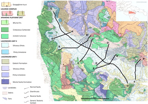
The basin infill consists of continental deposits up to 500 m thick and it is emplaced on the Southern Apennines NE-verging thrust-belt resulting from the Miocene–Early Pleistocene deformation of basin and shelf domains (Dewey et al. 1989; Patacca and Scandone 1989). The complex thrust-and-fold system has been deeply explored by commercial reflection profiles and wells (Menardi Noguera and Rea 2000; Dell’Aversana 2003; Shiner et al. 2004). In particular, hydrocarbon exploration shows that the shallow architecture derives from a poly-phase tectonic history (Menardi Noguera and Rea 2000; Shiner et al. 2004; Catalano et al. 2004). Since the Middle Miocene, thin-skinned tectonics was responsible for the build-up of a pile of rootless nappes, which has been drilled down to 2–4 km below the sea level. Mesozoic carbonates of the Western Carbonate Platform overthrust coeval pelagic sequences of the Lagonegro Basin (mainly consisting of cherty-limestones and cherts), which in turn tectonically overlay deeply deformed Mio-Pliocene foredeep deposits (Shiner et al. 2004). This stack of thrust-sheets overthrusted with an overall E-vergence shelf limestones of the Apulia Platform up to 7 km thick, which underwent thick-skinned tectonics during Late Pliocene–Early Pleistocene times (Menardi Noguera and Rea 2000). The detachment between the allochthon and the buried Apulian unit is marked by a mélange zone, generally several hundreds of meters thick and locally exceeding a kilometre in thickness (Shiner et al. 2004). From a mechanical point of view, the allochthonous and the Apulian units are characterized by a brittle behaviour, whereas the intermediate mélange zone shows ductile behaviour.

Pleistocene extensional tectonics combined with quaternary climate changes strongly controlled shape, morphology, and sedimentary evolution of the HAV basin up to the present (Giano et al. 1997, 2000; Schiattarella et al. 2003; Boenzi et al. 2004; Colella et al. 2004; Zembo 2010). The most recent studies suggest that the present-day basin configuration is due to phases of transtension and extension, between the Early Pleistocene and the Holocene, along two branching high-angle fault systems (Figure 2): the SW-dipping and NW–SE trending normal fault system located along the north-eastern flank of the basin (‘Eastern Agri Fault System’, Cello et al. 2003) and the eastern branch of the NE-dipping NW–SE striking normal fault system, located along the southern flank of the basin (‘Monti della Maddalena Fault System’, Maschio et al. 2005).

Figure 2. Quaternary deposits of the High Agri basin and stratigraphic relationships among them. Val d'Agri Fault System (EAFS; Cello et al. 2003); Monti della Maddalena Fault System (MMFS; Maschio et al. 2005). Pre-quaternary bedrock is not shown. Modified from Zembo et al. (2011).

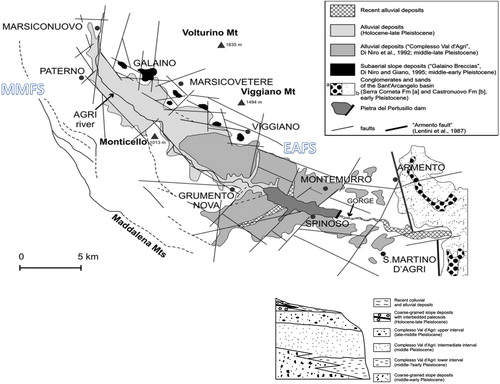
The genesis of the HAV basin can be schematically summarized in two main tectonic phases (Giano et al. 1997; Schiattarella et al. 1998; Schiattarella et al. 2003). The Late Pliocene–Early Pleistocene tectonic phases of the Southern Apennines, result from strike-slip movements along roughly NNE–SSW trending, right-lateral, and WNW–ESE trending, left-lateral, structures (Turco and Malito 1988; Ortolani et al. 1992; Cello et al. 2003; Shiner et al. 2004). The second phase takes its place in the Middle Pleistocene as a consequence of a regional-scale extensional regime with a NE–SW-oriented axis, resulting in NW–SE striking high-angle normal faults, which determined the enlargement and subsidence of the basin (Schiattarella 1998; Cello et al. 2003; Boenzi et al. 2004). Different stress indicators (Cello et al. 2003; Montone et al. 2004) instead suggest that this NE–SW extensional stress regime is ongoing, as inferred by the regional seismicity characterized in the recent past by frequent earthquakes and great magnitude, such as that of 1857 (Gasperini et al. 1999; Burrato and Valensise 2008), and as proved by the occurrence of paleosoils (ages between 40 and 20 ka) affected by normal faulting with pluridecimetric and metric cumulative displacements (Giano et al. 2000).

The HAV quaternary syntectonic continental deposits (Zembo 2010), influenced by the two main tectonic phases described above, consist essentially of (Figure 2):

• Lower–Middle Pleistocene talus breccia (‘Brecce di Galaino and Marsicovetere’ and ‘Brecce di Serra Mare’, Di Niro and Giano 1995; Giano et al. 1997; Boenzi et al. 2004), which are exposed only along the north-eastern and the south-western basin flank;

• Middle–Upper Pleistocene fluviolacustrine sediments (Val d'Agri Complex, Di Niro et al. 1992; Giano et al. 2000), and Upper Pleistocene–Holocene fluviolacustrine deposits.

The ages of the quaternary sediments have been inferred by correlating the polygenetic land surfaces of the HAV with post-Sicilian morphostratigraphic features from the nearby Sant'Arcangelo Pliocene–Pleistocene basin (Di Niro et al. 1992).

The Lower–Middle Pleistocene tilted and faulted slope deposits are characterized by roughly stratified breccias with reddish matrix, locally up to 20 ± 3 m thick, which are strongly deformed (first tectonic stage), separated from their source area and not connected with the alluvial plain (Giano et al. 2000).

The Val d'Agri Complex, only mildly faulted, was divided by Di Niro et al. (1992) to three lower rank units, forming an overall coarsening-upward sequence: the lower interval (Lower?–Middle Pleistocene), mainly silty clay and silt, shows local conditions of poor drainage (fluvial–lacustrine and overbank deposits). The other two intervals (Middle–Late Pleistocene), with gradual appearance of sands, gravels and conglomerates, show a reorganization of the hydrographic network (alluvial plain and proximal fan deposits).

According to Bianca and Caputo (2003), during the last uplift phase of lifting of the Middle–Upper Pleistocene, the morphostructural threshold placed at the anticline of the Armento allowed the formation of the Pertusillo paleolake and the beginning of the sedimentation of the Val d'Agri Complex (Di Niro et al. 1992). The incision of the threshold by the River Agri due to regressive erosion induced by the regional uplift causes the progressive emptying of the lake and the partial incision of the same fluvio-lacustrine deposits of the Val d'Agri Complex (Di Niro et al. 1992). According to Boenzi et al. (2004) and Schiattarella et al. (2006), the beginning of the fluvial incision of the basin threshold is due to a regional tectonic event, occurring at ca. 0.125 Ma.

The depositional top of the Val d'Agri Complex is deeply incised by the Agri River and its tributaries, only in the southern sector of the HAV, as a consequence of deepening of the drainage network, forming a wide terraced surface (Middle–Late Pleistocene terrace by Bianca and Caputo, 2003). Here, the Agri River leaves the HAV through a deep gorge (Pietra del Pertusillo) cut into the Miocene Gorgoglione flysch.

The uppermost Pleistocene and the Holocene sediments are represented by terraced alluvial sediments, alluvial fans and recent and present-day alluvial deposits; the recent alluvial sediments of the Agri River mostly crop out in the central and northern side of the basin, the latter displaying a flat morphology typical of an alluvial bottom valley. The younger fluvial terraces are telescoped into the deeply entrenched drainage network. After building of the Pertusillo dam (1957–1962), all the Holocene valleys at north of the artificial lake became oversupplied, with cycles of deposition/erosion of sands and gravels, modulated by the artificial lake level.

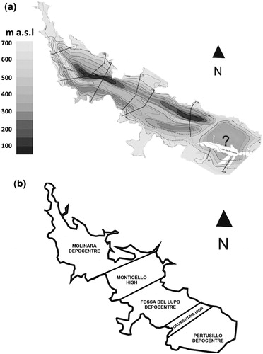
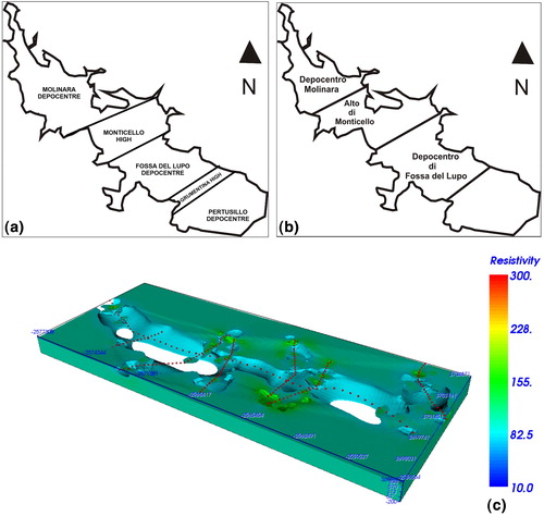
According to Colella et al. (2004) and Rizzo et al. (2004a), the deep architecture of the HAV, reconstructed by integrating geophysical and stratigraphic data, consists of three main tectonically controlled depocentres separated by two structural highs bounded by NE-oriented faults and by EAFS and MMFS fault systems (Figure 3). From NW to SE, the structure of the HAV comprises the following elements: Molinara depocentre, Monticello High, Fossa del Lupo depocentre, Grumentina High, Pertusillo depocentre. In the three depocentres, the thickness of the basin fill strongly varies, decreasing south-eastwards: the Molinara and Fossa Del Lupo depocentres are the most important and the quaternary sediment fill could reach a thickness >500 m; the Pertusillo depocentre strongly differs from the previous ones and the basin fill could not exceed 100 m. In general, the thickness of the sediments is very variable and decreases towards the south.

Figure 3. Sketch of the complex structural basin of the High Agri Valley as inferred from geophysical and geological data (Colella et al. 2004). (a) altitude above sea level of the top of the pre-quaternary bedrock of the High Agri Valley basin (black lines are the ERT profiles); (b) deep architecture of the High Agri Valley consisting in three main depocentres separated by two structural highs.

In detail, the pre-quaternary basin substrate consists of:

• Mesozoic-Tertiary carbonates with a neritic facies of escarpment, i.e. limestone and dolomites deposited in a protected and shallow environment (Unit of Monte Marzano-Maddalena Mounts, Bonardi et al. 1988), mainly outcropping along the western side of the basin;

• Lagonegro units rocks. They crop out mainly along the eastern flank of the valley and in sparse tectonic windows beneath the Maddalena Mounts thrust sheet in the western side;

• Toward the east and southeast, the pre-quaternary substratum consists of, Miocene siliciclastic sediments (Albidona and Gorgoglione flysch) that crop out mainly in the southern part of the HAV.

3. Methods

To improve the previous geophysical results on the pre-quaternary bedrock and the quaternary alluvial deposits, a 21 km-long DERT was carried out by reaching the investigation depth of about 1 km along the longitudinal section of the HAV basin.

Geoelectrical method is one of the geophysical methods that studies the electrical distribution properties in subsurface. The response is based on the measurement of electrical potential field on the surface that occur either naturally or due to the injection of an electric current into the earth. Some of geoelectrical method are SP and resistivity methods.

The basic principle of resistivity method is to inject a current (I, A) into the earth using two current electrodes A and B, then measure the potential difference ΔV (mV) through two other electrodes M and N on the surface of the earth, giving us a way to measure the electrical resistivity of the subsurface material. The measured apparent resistivity is a function of the measured impedance (ratio of electric potential in mV to current in A) and the geometry of the electrode array (K). In the shallow subsurface, the presence of water strongly controls the conductivity. Measurement of resistivity is, in general, a measure of water saturation and connectivity of pore space. This is because water has a low resistivity and electric current will follow the path of least resistance. Increasing saturation, increasing salinity of the underground water, increasing porosity of rock (water-filled voids) and increasing number of fractures (water-filled) all tend to decrease measured resistivity. Increasing compaction of soils or rock effectively increase resistivity. Air, with naturally high resistivity, results in the opposite response compared to water when filling voids. Whereas the presence of water will reduce resistivity, the presence of air in voids should increase subsurface resistivity.

2D ERT measures both the lateral and vertical variations of the electrical resistivity of the rocks, by moving current and potential electrodes and increasing their spacing along a chosen profile. The remarkable resolution obtained through this technique allows to discriminate, in a more effective way, resistivity contrasts present in the subsoil, providing information on the physical conditions of the rocks, on the presence of tectonic and/or stratigraphic discontinuity surfaces and on the presence of aquifers and/or fluids of various origins (Grahame 1947; Sato and Mooney 1960; Davis et al. 1978; Revil and Pezard 1998, 2003; Rizzo and Piscitelli 2007; Jouniaux 2011).

Resistivity measurements are associated with varying depths depending on the separation of the current and potential electrodes in the survey, and can be interpreted in terms of a lithological and/or geohydrological model of the subsurface. Measured data are termed apparent resistivity because the resistivity values measured are averages over the total current path length but are plotted at one depth point for each potential electrode pair. 2D images of the subsurface apparent resistivity variation are called pseudosections. Data plotted in cross-section are a simplistic representation of actual, complex current flow paths. Inversion software helps to interpret geoelectrical data in terms of more accurate earth models.

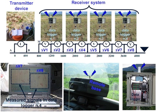
The realization of a DERT consists investigating electrical resistivity distribution at greater depth (>200 m) by using a physically separated system between the current injection (I) and the drop of potential measurements tools (ΔV). Usually for deep geoelectrical investigation, the current and potential electrodes placed on the ground are arranged with dipole–dipole (DD) electrode configuration (Figure 4). In DD array, all four electrodes are put at measurable distances from each other. In this array, both current electrodes are next to each other at distance a, while the potential electrodes are also next to each other at distance a and separated from the current electrode pair at a distance n. Therefore, the apparent resistivity is calculated (Hannenson 1990): (1) $$\rho =\left[\pi an\left(n+1\right)\left(n+2\right)\right]\left(\frac{\Delta V}{I}\right).$$(1)

Figure 4. Device system with transmitter and receiver units physically separated.

The advantage of the DD with respect to the other electrode configurations lies in the fact that the distance between the measuring electrodes and the current ones is limited only in the sensitivity of the instruments and in the background noise. Therefore, it is more suitable for deep investigations (>200 m) otherwise not to be tackled with quadripolar configuration.

The electric potential signal to be measured could be sometimes very low depending on the intensity of the current input, on the subsoil electrical characteristics and on the electrode distances. In fact, for large distances between the AB and MN electrodes, the measured electric potential is sometimes lower, which is due to disturbing currents present in the ground, such as industrial, telluric and inductive currents (between cables), which may occur when the energizing circuit is activated.

The drop of potential ΔV(t), measured at the MN electrodes, can be represented by the following relation: (2) $$\Delta V\left(t\right) =S\left(t\right) +N\left(t\right)$$(2)

where S(t) represents the useful signal and N(t) symbolizes the noise.

However, the quality of the signal also depends on the spacing between electrodes, worsening as the receiving dipole moves away from the energizing one. The distribution of conductivity in the soil also affects the quality of the signal; in fact, in highly conductive areas, located between the transmitting and receiving dipoles, the electric potential is strongly masked to such an extent that the signal is completely erased from the background noise. Furthermore, geoelectrical data acquisition in urbanized areas is characterized by a greater noise level because of the disturbances due to environmental noise. For all these reasons, the voltage signal useful for obtaining the essential information to calculate the apparent resistivity could be hidden.

To obtain a 2D real resistivity model of subsoil, the apparent resistivity values should be inverted by means of the inversion algorithms. There are several approaches of 2D inversion and for our data, we used three different types: RES2Dinv by Geotomo Software (LOKE e BARKER, 1996), where the inversion routine is based on the smoothness constrained least-squares inversion implemented by a quasi-Newton optimisation technique; DCIP2D by UBC-GIF (Oldenburg et al. 1993), which consists of iterative procedures of systems of equations based on objective functions; ZondRes2D software (Zond geophysical software), which is a computer program for 2.5D interpretation of ERT and finite-element method as mathematical apparatus is used to solve forward and inverse.

4. Field data acquisition

To identify the best surface electrical dipoles position and therefore optimize both the geophysical data acquisition time and results, we individuated, following a site inspection, 53 point (red tacks in Figure 5) possibly representing the surface dipole electrodes position for deep electrical resistivity measurements. They were chosen taking into account the ease of reaching the place with the geophysical equipment and the absence of any natural and anthropogenic limits for power cables roll out.

Figure 5. Geolocated stations of the new 2D DERT.

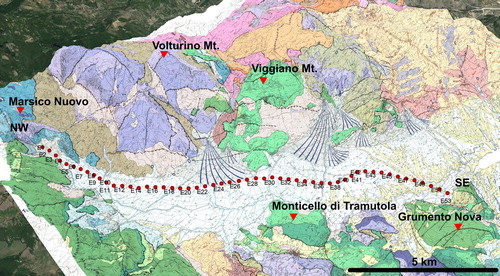
Following the site inspection, a deep geoelectrical tomography with NW–SE trend was carried out along a wide portion of the HAV between Marsico Nuovo and Grumento Nova towns.

In particular, a system conceived and realized at the Geophysical Laboratory of CNR-IMAA was used. The instrumentation is divided into two parts: an energizing system and a receiving one.

The energizing system consists of a current injection transmitter connected to an adequate power system used to introduce an electric current into the ground through current electrodes A and B. The choice of the type of power system was weighted considering a series of factors such as the depth of investigation, the soil characteristics, the environmental electrical noise, etc. To ensure a good electrical contact, we used current electrodes with a diameter of 20–30 mm and a length of 1 m. Furthermore, in each current station (A and B position) three connected electrodes were used, to reduce the surface resistance and improve the current injection. The electrode distance was 400-m long. To energize direct current, the addition of a current rectifier to transform the alternating voltage into direct voltage was required. Finally, the energization system displays how many electrical current is injected in the subsoil. Therefore, an operator recorded the values at regular intervals of 2 min, since the current pulse was rather stable.

The receiving system measures the generated voltage signals (ΔV) between potential electrodes MN. Drop of potential values are recorded with a regular sampling step (1 s), chosen to fit an integer number of times in the full cycle of a current wave. In particular, the used receiving system consists of unpolarizable electrodes driven into the ground connected to a multichannel receiver system made of four remote multichannel dataloggers, radio-connected to a personal computer, simultaneously recording up to 32 drop of potential (mV). In this work, we used only four channels for each datalogger, to collect at the same time eight drops of potential for each dipole current injection. Unpolarizable electrodes were necessary to obviate the problem of ‘electrode polarization’, a source of noise which, if present, alters the survey data considerably.

Furthermore, single-core, flexible, low-ohmic copper cables were used; the choice of their section depends on the maximum amount of current that the generator is able to supply; they must be wound on suitable cable reels to facilitate both transport and unwinding and rewinding.

This type of instrumentation appears to be at the forefront of geophysical surveys, bringing numerous innovations compared to the instrumentation used in the past. Furthermore, it allows to expand and adapt the system to the most varied logistic conditions, both as regards the number of data that can be acquired (increasing considerably the number), and in optimizing the investigation times, managing to acquire, at the same length, a tomography in half the time.

Finally, in previous measurement campaigns (Colella et al. 2004; Rizzo et al. 2004a), it was possible to use a maximum electrodes spacing of 200 m, while the new acquisition system allows to use electrodes spacing of about 400 m.

In particular, a 40 s lasting electric signal in the form of a square wave, with a maximum current of 10 A, was injected into the ground. The DD array used was characterized by a = 400 m (electrodes spacing) and a maximum of 8a. The total maximum distance between the energizing and receiving stations was of 4000 m. The data records have lasted from 10 to 20 min, to have a sufficient number of square waves cycles to allow the extraction of the useful signal from the background noise. A sampling rate of one second was chosen. At the end of the survey a total of 351 potential measurements were recorded along a 20,800 m-long profile.

The geoelectrical survey lasted about a month, considering the length of the tomography (20,800 m) that was acquired. For the acquisition, it was necessary to use a group of 5/6 people distributed among the four dataloggers, the energizing system and the person in charge of displaying the voltage values to the portable computer. Usually, the most distant receiving stations suffer from a greater reduced signal/noise ratio, therefore the person in charge of reading the signal to the PC checked if the data recording voltage drop were satisfactory by controlling more closely the electrical potential cycles measured.

5. Data analysis and inversion

The huge work in the field permitted to acquire several data (current and drop of potential) during the geophysical surveys. Therefore, an analytical protocol was necessary for data analysis.

In shallow investigations, a routine statistical analysis of voltage signals is sufficient to reduce the errors associated to the estimate of the potential values. On the contrary, in deep geoelectrical explorations a crucial task is the extraction of useful signal from voltage recordings. In fact, the large distance between the energizing and receiving systems strongly reduces the signal-to-noise ratio. To overcome this drawback, for each electrode position the corresponding voltage signals was filtered, stored and processed. Taking into account that the signal-to-noise ratio depends from the distance between the current emitters and receivers, the success of the methodology is related to the duration of voltage recordings. The rationale of field acquisition and processing was to record voltage data for enough time so as to always have sufficient number of cycles to extract the amplitude of the signals from the background noise.

For this effort, we used OriginPro software (OriginLab Corporation) where graphing and data analysis tools were used (Figure 6). In details, the following tools were applied: spike removing, plot analysis polynomial or linear fit, de-trending, FFT signals processing of voltage. The first step of the voltage data analysis was the spike removing, which consists to delete the spikes on the active graph window. The second step was the de-trending analysis, which consisted in a polynomial or linear fit of the voltage data and a subsequently de-trend approach, in order to remove the natural trend that enveloped the data (Figure 6(a–c)). Successively, a FFT tool was performed to the de-trending voltage data (Figure 6(d)). The FFT analysis converts a signal from its original time domain to a representation in the frequency domain. Meanwhile, it can also provide the magnitude, amplitude, phase, power density and other computation results. In our case, the amplitude of the FFT results in the frequency of the acquired current signal defines the amount of the drop of potential. In the case in which recorded voltages were characterized by a good signal-to-noise ratio, in the spectrum of signal amplitudes we will have a peak right at the energization frequency (which in our case was equal to 0.025 Hz). On the contrary, the spectrum of particularly noisy voltage signals presented a series of ‘spikes’ that make the identification of the useful signal much more complex (Figure 6(e,f)).

Figure 6. (a) Example of Fourier analysis applied to a signal recording in which there is a (b) polynomial type trend that was removed. (c) Application of Fourier analysis to an example of signal recording with a good signal-to-noise ratio. (d) The peak at the energization frequency (0.025 Hz). Application of the Fourier analysis to (e) an example of signal recording with a very low signal-to-noise ratio. (f) The main peak is not at the energization frequency.

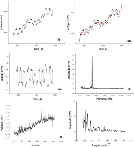
After the analysis and elaboration steps, about 16 potential data were rejected because of the potential signal was not visible; however, considering only the good data, a 335 resistance values (V/I, Ω) were estimated taking in account the extrapolated potential data and the injected current. Therefore, it was possible to define the apparent resistivity data plotted in a 2D image from the resistance and the geometric factor. The next step defines the real electrical resistivity distribution by the inversion phase of all the apparent resistivity values. The inversion and optimization processes of the recorded values along the long longitudinal profile have been executed by means of different inversion programme but we show only the results coming from the ZondRes2D software (Zond geophysical software). It is a computer program for 2.5D interpretation of ERT and finite-element method as mathematical apparatus is used to solve forward and inverse. The first step was to prepare the data for the inversion, such as poor data detection. The next step was to select the inversion type and parameters. In order to transform the apparent resistivity pseudosection into a model representing the distribution of calculated electrical resistivity in the subsurface, we used the smoothness constrained that is an inversion by least-square method with use of smoothing operator. The inversion type was Marquardt classic inversion algorithm consisted in a least-square method with regularization by damping parameter (Marquardt 1963). In case of little quantity of section parameters, this algorithm allows receiving contrast subsurface model

Finally, in order to obtain a real 3D resistivity model of the HAV, new and previous apparent electrical resistivity data acquired by Colella et al. (2004) were inverted using ERTlab (Geostudi Astier srl and Multi-Phase Technologies LLC). ERTLab is a resistivity inversion software that offers full 3D modelling and inversion. Its numerical core use finite elements (FEM) approach to model the subsoil by adopting a mesh of hexahedrons to correctly incorporate complex terrain topography. Moreover, the software inverts data-sets collected using surface, borehole or surface-to-hole array configurations. The true resistivity distribution is estimated by minimizing the chi-squared function: (3) $${\chi }^2=\sum \left(\frac{{\rho }_m-{\rho }_c}{{\sigma }_i}\right)$$(3)

where, respectively, σ_i is the estimated data variance; ρ_m and ρ_c are the ith value of the measured and calculated apparent resistivity for the same quadrupole. The inversion procedure is based on a smoothness constrained least-squared algorithm (LaBrecque et al. 1999) with Tikhonov model regularization, where the condition of the minimum roughness of the model is used as a stabilizing function. Throughout the inversion iterations, the effect of non-Gaussian noise is appropriately managed using a robust data-weighting algorithm (Morelli and LaBrecque 1996).

The total data set (882 measurements) was inverted by using a mesh with more than 300.000 tetrahedral cells (200 × 200 × 50 m³), a mixed boundary condition (Dirichlet and Neumann), and a starting homogeneous apparent resistivity of 100 Ω*m. Both core and boundary mesh were generated to accommodate boundary conditions. A 2% standard deviation estimate for noise was assumed to invert the data set with a robust inversion. The inversion time lasted about 3 h.

6. Results and discussion

Figure 7 shows the result of the 2D DERT reaching an investigation depth >1000 m b.g.l. The resistivity model is characterized by resistivity values varying from 10 Ω*m to over 900 Ω*m. It is generally possible to observe a large, relatively conductive area (<100 Ω*m) distributed for the whole tomography with inside more conductive areas (<10 Ω*m). Moreover, a very resistive body (>500 Ω*m) is observed, extended for over 5 km length, located from about 9500 to 1600 m from the beginning of the profile and placed at a depth of about 200 m b.g.l. In addition, from 4500 to 7000 m at a depth of about 800 m b.g.l., a resistive zones (>300 Ω*m) is observed, alternating with relatively conductive areas (<100 Ω*m).

Figure 7. The 2D DERT image after the inversion with topography correction.

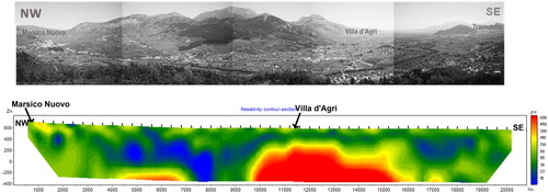
By comparing the new 2D electrical resistivity results with previous geophysical, geological, and stratigraphic data present in the literature, is it possible to obtain information on the structure at depth of the basin. In particular, the resistivity values of the tomography can be interpreted as follows: the pre-quaternary substrate is characterized by resistivity values >300 Ω*m, while, quaternary sediments are characterized by resistivity values <100 Ω*m.

The strong resistivity contrast between alluvial deposits and the pre-quaternary substrate highlights the complex geometry of the basin. Data inversion allowed us to understand the transition between the pre-quaternary substratum and the alluvial sediments, so as to characterize the superficial morphology of the pre-quaternary bedrock. From these new data result that the thickness of the sedimentary filling varies considerably, from the northernmost part of the tomography going towards the southern area, reaching thicknesses of over 1 km. The minimum thickness of the quaternary sediments (about 200 m) can be observed at the large block of pre-quaternary substratum, in the central sector of the basin, close the Villa d’Agri town.

Figure 8 shows the 3D electrical resistivity image of the HAV basin obtained with all the collected electrical resistivity data. The resistivity values of the 3D inversion model show a lowest range then the 2D inversion model. On the contrary, the resistivity contrast is well defined in both models, correlating with the geological interpretation. The 3D electrical model has a volume type visualization where the low electrical resistive area (<100 Ω*m), associated to the quaternary basin, is well distinguished along the valley and on its flanks. Moreover, the 3D electrical image highlights also the different depth of the basin.

Figure 8. (a) The 3D electrical resistivity image obtained by ERTLab inversion software. The image highlights the low resistivity zone of the Val d’Agri basin (<50 Ω*m) and the high resistivity zone of the central part of the tomography. (b) The misfit graph of the last interactions (n.4).

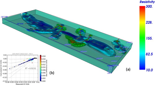
This result allowed revisiting the interpretation of Colella et al. (2004) about pre-quaternary substratum geometry (Figure 9). In particular, the area between the NW extreme of the tomography up to 9600 m, can be associated to the Molinara depocentre with sediment thickness of >1 km. The area between 9600 to about 15,000 m, can be associated with the Monticello high, where there is the minimum thickness of the quaternary sediments. Instead, the southernmost area of tomography is associated with the Fossa del Lupo depocentre where the quaternary deposits reach a minimum thickness of 800 m.

Figure 9. New interpretation of High Agri Valley pre-quaternary substratum geometry according to (a) Colella et al. (2004) and (b) the new geophysical data interpretation. (c) The 3D electrical resistivity image without the low resistivity zone of the quaternary basin, highlighting the different depocenters and highs.

In particular, the buried structural highs are bordered by anti-Apennine faults, probably characterized by a strike-slip component and the Monticello structural high (Collella et al. 2004) may correspond to the carbonate block of Viggiano Mt., located along the Southeastern flank of the basin. It is finally possible to state, on the basis of geological constraints, that the presented geological setting was entirely formed during the Early Pleistocene. In particular, these constraints are based on the age of the Val d'Agri Complex filling.

7. Conclusions

A new 2D DERT has been realized longitudinally to the HAV basin, with a NW-SE trend, from the Marsico Nuovo to Grumento Nova towns. The new DERT has a total length of 20,800 m, a depth of investigation of about 1 km, an electrode spacing of 400 m, a total of 53 stations, and 351 voltage signal recordings.

The new resistivity data were inverted by a 3D software to integrate even old resistivity data measured in the HAV by Colella et al. (2004).

With the contribution of available geological and geophysical data our new geophysical results allow us to make a further scientific contribution to the study of the intermontane basin of the HAV.

The complex evolution of the HAV basin, due to its structure in blocks, with intrabasinal highs and lows, has meant that the thickness of the infill deposits varies considerably both in the transverse and longitudinal directions. The subdivision into blocks, characterized by depocentres and structural highs, proposed by Colella et al. (2004), obtained through the elaboration of geophysical and geological-stratigraphic data, can be confirmed, however the greater detail obtained from the longitudinal electrical resistivity measurements, allowed us to more precisely locate the boundaries of the Molinara and Fossa del Lupo Depocentres, and of the Monticello High.

So it is possible to state that the Molinara Depocentre, Monticello High and Fossa del Lupo Depocentre extend for about 9, 5 and 6 km respectively.

Moreover, it is possible to observe from the results obtained in this work that the thickness of the basin sediments, which according to Colella et al. (2004) reached its maximum in the Molinara depocentre, equal to about 500 m, is instead >1 km in the same depocentre. As for the of Fossa del Lupo depocentre, it is possible to assert that the thickness of the sediments is about 700 m, while obviously the sediments reach the minimum thickness in the upper part of Monticello High.

Acknowledgements

We wish to thank the student, Maria Carmela Miraglia, of the University of Basilicata for her contribution on this work during her bachelor’s degree. Moreover, the authors thank all the people who went in field for the long data acquisition (Gregory De Martino, Giuseppe Calamita, Marianna Balasco, Luigi Capozzoli). The authors thank Federico Frishanger (Geostudi Astier) for his help on the 3D inversion by ERTLab software. Finally, Enzo Rizzo thanks the director of the CNR-IMAA, Dr. Vincenzo Lapenna, for his continue support to Hydrogeosite Laboratory research activities. Finally, the authors thank the two anonymous reviewers who help us to improve the paper.

Disclosure statement

No potential conflict of interest was reported by the author(s).

References

- Balasco M, Galli P, Giocoli A, Gueguen E, Lapenna V, Perrone A, Piscitelli S, Rizzo E, Romano G, Siniscalchi A, et al. 2011. Deep geophysical electromagnetic section across the Middle Aterno Valley (Central Italy): Preliminary results after the April 6, 2009 L’Aquila Earthquake. Bollettino di Geofisica Teorica ed Applicata. 52(3):443–455.
- Balasco M, Giocoli A, Piscitelli S, Romano G, Siniscalchi A, Stabile TA, Tripaldi S. 2015. Magnetotelluric investigation in the High Agri Valley (Southern Apennine, Italy). Nat Hazards Earth Syst Sci. 15(4):843–852.
- Beckers A, Hubert-Ferrari A, Beck C, Bodeux S, Tripsanas E, Sakellariou D, De Batist M. 2015. Active faulting at the western tip of the Gulf of Corinth, Greece, from high-resolution seismic data. Mar Geol. 360:55–69.
- Beilecke T, Krawczyk CM, Ziesch J, Tanner DC. 2016. Near-surface fault detection using high-resolution shear wave reflection seismics at the CO2CRC Otway Project site, Australia. J Geophys Res Solid Earth. 121(9):6510–6532.
- Beka TI, Bergh SG, Smirnov M, Birkelund Y. 2017. Magnetotelluric signatures of the complex tertiary fold–thrust belt and extensional fault architecture beneath Brøggerhalvøya, Svalbard. Polar Res. 36(1):1409586.
- Bertello F, Fantoni R, Franciosi R. 2008. Exploration country focus: Italy. AAPG–ER Newsletter, June 2008, 5–9.
- Bertello F, Fantoni R, Franciosi R, Gatti V, Ghielmi M, Pugliese A. 2010. From thrust-and-fold belt to foreland: hydrocarbon occurrences in Italy. Pet Geol Conf Ser. 7(1):113–126.
- Bianca M, Caputo R. 2003. Analisi morfotettonica ed evoluzione quaternaria della Val d’Agri, Appennino Meridionale, Il Quaternario. 16(2):159–170.
- Boenzi F, Capolongo D, Cecaro G, D’Andrea E, Giano SI, Lazzari M, Schiattarella M. 2004. Evoluzione geomorfologica polifasica e tassi di sollevamento del bordo sud-occidentale dell’alta Val d’Agri (Appennino meridionale). Boll Soc Geol It. 123:357–372.
- Bonardi G, D’Argenio B, Perrone V. 1988. Carta Geologica dell’Appennino Meridionale alla scala 1:250.000, Mem. Soc Geol It. 41:13–41.
- Boncio P, Milana G, Cara F, Di Giulio G, Di Naccio D, Famiani D, Liberi F, Galadini F, Rosatelli G, Vassallo M. 2016. Shallow subsurface geology and seismic microzonation in a deep continental basin. Avezzano town, Fucino basin (central Italy). Nat Hazards Earth Syst Sci Discuss.
- Burrato P, Valensise G. 2008. Rise and fall of a hypothesized seismic gap: source complexity in the 16 December 1857, Southern Italy earthquake (Mw 7.0). Bull. Seism. Soc. Am. 98(1):139–148.
- Buttinelli M, Improta L, Bagh S, Chiarabba C. 2016. Inversion of inherited thrusts by wastewater injection induced seismicity at the Val d’Agri oilfield (Italy). Sci Rep. 6(1):37165.
- Caputo R, Piscitelli S, Oliveto A, Rizzo E, Lapenna V. 2003. High-resolution resistivity tomographies in active tectonic studies. Examples from the Tyrnavos Basin, Greece. J Geodin. 36(1–2):19–35.
- Carbone S, Catalano S, Lazzari S, Lentini F, Monaco C. 1991. Presentazione della carta geologica del bacino del Fiume Agri (Basilicata). Mem Soc Geol It. 47, 129–143.
- Catalano S, Monaco C, Tortorici L, Paltrinieri W, Steel N. 2004. Neogene-quaternary tectonic evolution of the Southern Apennines. Tectonics. 23(2):1–19.
- Cello G, Tondi E, Micarelli L, Mattioni L. 2003. Active tectonics and earthquake sources in the epicentral area of the 1857 Basilicata earthquake (southern Italy). J Geodyn. 36(1–2):37–50.
- Civico R, Sapia VD, Giulio G, Villani F, Pucci S, Baccheschi P, Amoroso S, Cantore L, Di Naccio D, Hailemikael S, et al. 2017. Geometry and evolution of a fault-controlled quaternary basin by means of TDEM and single-station ambient vibration surveys: the example of the 2009 L’Aquila earthquake area, central Italy. J Geophys Res Solid Earth. 122:2236–2259.
- Colella A, Lapenna V, Rizzo E. 2004. High-resolution imaging of the High Agri Valley Basin (Southern Italy) with electrical resistivity tomography. Tectonophysics. 386(1–2):29–40.
- Davis JA, James RO, Leckie JO. 1978. Surface ionization and complexation at the oxide/water interface. J Colloid Interface Sci. 63(3):480–499.
- Dell‘Aversana P. 2003. Integration loop of ‘global offset’ seismic, continuous profiling magnetotelluric and gravity data. First Break. 21(1006):32–41.
- Demanet D, Pirard E, Renardy F, Jongmans D. 2001. Application and processing of geophysical images for mapping faults. Comp Geosci. 27(9):1031–1037.
- Dewey JF, Helman ML, Turco E, Hutton DHW, Knott SD. 1989. Kinematics of the western Mediterranean. In: Coward MP, Dietrich D, Park RG, editors. Alpine tectonics. London: Geoloical Society London Special Publication. Vol. 45; p. 265–283.
- Di Maio R, Mauriello P, Patella D, Petrillo Z, Piscitelli S, Siniscalchi A. 1998. Electric and electromagnetic outline of the Mount Somma–Vesuvius structural setting. J Volc Geoth Res. 82(1–4):219–238.
- Di Niro A, Giano SI. 1995. Evoluzione geomorfologica del bordo orientale dell’alta Val d’Agri (Basilicata). Studi Geologici Camerti. 2:207–218.
- Di Niro A, Giano SI, Santangelo N. 1992. Primi dati sull’evoluzione geomorfologica e sedimentaria del bacino dell’alta Val d’Agri (Basilicata). Studi Geologici Camerti. 1:257–263.
- Gasperini P, Bernardini F, Valensise G, Boschi E. 1999. Defining seismogenic sources from historical earthquake felt reports. Bull Seism Soc Am. 89:94–110.
- Giano SI, Lapenna V, Piscitelli S, Schiattarella M. Nuovi 1997. dati geologici e geofisici sull'assetto strutturale dei depositi continentali quaternari dell'alta Val d'Agri (Basilicata). Il Quaternario. 10:591–596.
- Giano SI, Lapenna V, Piscitelli S, Schiattarella M. 2000. Electrical imaging and self-potential surveys to study the geological setting of the quaternary slope deposits in the Agri High Valley (southern Italy). Ann Geofis. 43:409–419.
- Giano SI, Schiattarella M. 2002. Geomorfologia e Neotettonica dell’alta Val d’Agri. In: Boenzi, F., Schiattarella, M., Guida all’Escursione Geomorfologica: dalla Val d’Agri a Matera. Potenza: Assemblea-EscursioneAIGeo; p. 22–34.
- Giocoli A, Magrì C, Piscitelli S, Rizzo E, Siniscalchi A, Burrato P, Vannoli P, Basso C. 2008. Di Nocera S.: electrical resistivity tomography investigations in the Ufita Valley (southern Italy). Ann. Geophys. 51:213–223.
- Grahame SA. 1947. The electrical double layer and the theory of electrocapillarity. Chem Rev. 41(3):441–501.
- Hallof PG. 1957. On the interpretation of resistivity and induced polarization measurements [Ph.D. thesis]. Cambridge: MIT.
- Hannenson JE. 1990. A model for interpreting IP/resistivity data from areas of steep dip and thin overburden. In: Fink JB., McAlister EO, Sternberg BK, Wieduwilt WG, Ward SH, editors. lnduced Plarization, Applications and case histories, series investigation in geophysics. Tulsa, USA: Society of Exploration Geophysicist; p. 421.
- Improta L, Bagh S, De Gori P, Valoroso L, Pastori M, Piccinini D, Chiarabba C, Anselmi M, Buttinelli M. 2017. Reservoir structure and wastewater-induced seismicity at the Val d’Agri oilfield (Italy) shown by three-dimensional Vp and Vp/Vs local earthquake tomography. J Geophys Res Solid Earth. 122(11):9050–9082.
- Improta L, Ferranti L, De Martini PM, Piscitelli S, Bruno PP, Burrato P, Civico R, Giocoli A, Iorio M, D'Addezio G, et al. 2010. Detecting young, slow-slipping active faults by geologic and multidisciplinary high-resolution geophysical investigations: a case study from the Apennine seismic belt, Italy. J Geophys Res. 115(B11):B11307.
- Jouniaux L. 2011. Electrokinetic techniques for the determination of hydraulic conductivity. In: Elango L, editors. Hydraulic conductivity – issues, determination and applications. London:In Tech Publisher.
- Karaş M, Tank SB, Özaydın S. 2017. Electrical conductivity of a locked fault: investigation of the Ganos segment of the North Anatolian Fault using three-dimensional magnetotellurics. Earth Planets Space. 69(1):107.
- Kolawole F, Atekwana EA, Laó-Dávila DA, Abdelsalam MG, Chindandali PR, Salima J, Kalindekafe L. 2018. High-resolution electrical resistivity and aeromagnetic imaging reveal the causative fault of the 2009 Mw 6.0 Karonga, Malawi earthquake. Geophys J Int. 213(2):1412–1425.
- LaBrecque D, Morelli G, Daily W, Ramirez A. 1999. Lundegard P.: Occam’s inversion of 3D electrical resistivity tomography. In: Oristaglio M, Spies B, Cooper MR, editors. Three-dimensional electromagnetics. Tulsa, Okla: Society of Exploration Geophysicists; p. 575–590.
- Marquardt DW. 1963. An algorithm for least squares estimation of nonlinear parameters. J Soc Indust Appl Math. 11(2):431–441.
- Maschio L, Ferranti L, Burrato P. 2005. Active extensional in Val d'Agri area, Southern Apennines, Italy: implications for the geometry of the seismogenic belt. Geophys J Int. 162(2):591–609.
- Mekkawi MM, Fergani ESA, Abdella KA. 2017. Seismic risk zones and faults characterization using geophysical data. J Geol Geophys. 6:311.
- Menardi Noguera A, Rea G. 2000. Deep structure of the Campanian – Lucanian Arc (Southern Apennine, Italy). Tectonophysics. 324(4):239–265.
- Montone P, Mariucci MT, Pondrelli S, Amato A. 2004. An improved stress map for Italy and surrounding regions (central Mediterranean). J Geophys Res. 109(B10):B10410.
- Morelli G, LaBrecque DJ. 1996. Advances in ERT inverse modeling. Eur J EEGS. 1:171–186.
- Nocentini M, Asti R, Cosentino D, Durante F, Gliozzi E, Macerola L, Tallini M. 2017. Plio-Quaternary geology of L’Aquila – Scoppito Basin (Central Italy). J Maps. 13(2):563–574.
- Oldenburg DW, Mcgillivray PR, Ellis RG. 1993. Generalized subspace method for large scale inverse problems. Geophys J Int. 114(1):12–20.
- Onnis L, Violante R, Osella A, de la Vega M, Tassone A, López E. 2017. Neogene-quaternary seismic stratigraphy of the Llancanelo Lake Basin, Mendoza, Argentina. Andgeo. 45(1):35–46.
- Ortolani F, Pagliuca S, Pepe E, Schiattarella M, Toccaceli RM. 1992. Active tectonics in the Southern Apennines: relationships between cover geometries and basement structure. Hypothesis Geodynamic Model. 5:413–419.
- Patacca E, Scandone P. 1989. Post-Tortonian mountain building in the Apennines. The role of the passive sinking of a relic lithospheric slab. In: Boriani A, Bonafede M, Piccardo GB, Vai GB, editors. The lithosphere in Italy, vol 80. Italy:Advances in Earth Science Research. Atti Convegni Lincei; p. 157–176.
- Pucci S, Civico R, Villani F, Ricci T, Delcher E, Finizola A, Sapia V, De Martini PM, Pantosti D, Barde-Cabusson S, et al. 2016. Deep electrical resistivity tomography along the tectonically active Middle Aterno Valley (2009 L’Aquila earthquake area, central Italy). Geophys J Int. 207(2):967–982.
- Revil A, Naudet V, Nouzaret J, Pessel M. 2003. Principles of electrography applied to self-potential electrokinetic sources and hydrogeological applications. Water Resour Res. 39(5):1114.
- Revil A, Pezard PA. 1998. Streaming electrical potential anomaly along faults in geothermal areas. Geophys Res Lett. 25(16):3197–8007.
- Rizzo E, Colella A, Lapenna V, Piscitelli S. 2004. High-resolution images of the fault-controlled High Agri Valley basin (Southern Italy) with deep and shallow electrical resistivity tomographies. Phys. Chem. Earth. 29(4–9):321–327.
- Rizzo E, Piscitelli S. 2007. La Tomografia Geoelettrica Profonda (DERT): applicazione nel bacino dell’Alta Val d’Agri. Akiris. 8–9:45–49.
- Rizzo E, Suski B, Revil A, Straface S, Troisi S. 2004. Self-potential signals associated with pumping tests experiments. J Geophys Res. 109(B10):B10203.
- Sato M, Mooney HM. 1960. The electrochemical mechanism of sulphide self-potentials. Geophysics. 25(1):226–249.
- Schiattarella M. 1998. Quaternary tectonics of the Pollino Ridge, Calabria-Lucania boundary, southern Italy. In: Holdsworth RE, Strachan RA, Dewey JF, editors. Continental transpressional and transtensional tectonics, vol. 135. London: Geological Society; p. 341–354.
- Schiattarella M, Di Leo P, Beneduce P, Giano SI. 2003. Quaternary uplift vs tectonic loading: a case study from the Lucanian Apennine, southern Italy. Quaternary Int. 101–102:239–251.
- Schiattarella MD, Leo P, Beneduce P, Giano SI, Martino C. 2006. Tectonically driven exhumation of a young orogene: an example from the Southern Apennines. Italy: Geological Society of America Special Paper (398); p. 371–385.
- Schiattarella M, Ferranti L, Giano SI, Maschio L. 1998. Evoluzione Tettonica Quaternaria dell'Alta Val d'Agri (Appennino meridionale). In: 79° Congresso della Società Geologica Italiana, Palermo, September 21–23.
- Seminsky KZ, Zaripov RM, Olenchenko VV. 2016. Interpretation of shallow electrical resistivity images of faults: tectonophysical approach. Russ. Geol. Geophys. 57(9):1349–1358.
- Shiner P, Beccacini A, Mazzoli S. 2004. Thin-skinned versus thick-skinned structural models for Apulian carbonate reservoirs: constrains from the Val d’Agri Fields, S Apennines, Italy. Mar Pet Geol. 21(7):805–827.
- Stabile TA, Giocoli A, Perrone A, Piscitelli S, Lapenna V. 2014. Fluid injection induced seismicity reveals a NE dipping fault in the south-eastern sector of the High Agri Valley (southern Italy). Geophys Res Lett. 41:5847–5854.
- Steeples DW. 2001. Engineering and environmental geophysics at the millenium. Geophysics. 66(1):31–35.
- Storz H, Storz W, Jacobs F. 2000. Electrical resistivity tomography to investigate geological structures of the earth’s upper crust. Geophys Prospect. 48:455–471.
- Suzuki K, Toda S, Kusunoki K, Fujimitsu Y, Mogi T, Jomori A. 2000. Case studies of electrical and electromagnetic methods applied to mapping active faults beneath the thick quaternary. Eng Geol. 56(1–2):29–45.
- Turco E, Malito M. 1988. Formazione di bacini e rotazione di blocchi lungo faglie trascorrenti nell’Appennino meridionale. Riassunti 74° Congr. Soc. Geol. It., Sorrento.
- Tün M, Pekkan E, Özel O, Guney Y. 2016. An investigation into the bedrock depth in the Eskisehir Quaternary Basin (Turkey) using the microtremor method. Geophys J Int. 207(1):589–607.
- Van Dijk JP, Bello M, Toscano C, Bersani A, Nardon S. 2000. Tectonic model and three-dimensional fracture network analysis of Monte Alpi (Southern Apennines). Tectonophysics. 324(4):203–237.
- Zembo I. 2010. Stratigraphic architecture and quaternary evolution of the Val d’Agri intermontane basin (Southern Appennines, Italy). Sediment Geol. 223(3–4):206–234.