Multi-temporal analysis of morphologic changes applying geomatic techniques. 70 years of torrential activity in the Rebaixader catchment (Central pyrenees)

Abstract

The monitoring of morphologic changes in high-mountain environments is an important, but complex task. Terrestrial as well as airborne laser scanning (TLS and ALS) and digital photogrammetry (DP) using Unnamed Aerial Vehicle (UAV) can determine recent variations. In contrast, changes that occurred 20 or more years ago, need generally the application of DP and historic aerial photograph. We compared these four geomatic techniques and the resulting digital elevation models (DEM) that ranged over a 70-year time span (1946–2016). The accuracy of the different models and also the effect of different cell size were analysed. The accuracy analysis of the resulting DEMs shows important drawbacks, when historic aerial photographs are used. In these DEMs, the error in elevation can be important and a detailed analysis of morphologic changes is limited. Nowadays, the combination of DP and UAV is the technique with best cost-benefit ratio, although TLS could reveal similar precision. However, the application of TLS is restrained by the complex morphology and the presence of vegetation, which produce many shadows. Finally, the erosion rate was determined in our catchment. The resulting values range between 0.06 and 0.16 m³/m²/y, which coincides rather well with data observed in other studies.

Keywords:

• Digital photogrammetry
• TLS
• ALS
• UAV
• erosion rate
• Pyrenees

1. Introduction

The importance of monitoring topographic changes associated with geomorphologic processes has increased during the last decades (Bennett et al. 2012; Jaboyedoff et al. 2012; Kamps et al. 2017). Assessment and mitigation of geomorphologic hazards and risks have improved quality due to technological advances in geomatic surveys, but still need to resolve multiples difficulties. When the observation focuses on mass movements in high mountain regions or on torrential processes, the situation is even more complex because of the fact that study sites are mostly located in remote areas with steep slopes; very irregular terrain and the significant amount of vegetation (Blasone et al. 2014; Zhang et al. 2015; Fey and Wichmann 2017).

Since roughly 20 years ago, geomatic techniques allow the observation of ground movements using control points total stations or GNSS systems (Sanjosé-Blasco et al. 2007). During the last decades, methods have strongly improved including different types of technologies: i) higher resolution of satellite images (Liberti et al. 2009), ii) photogrammetry analysing historical aerial photographs or multiple digital images (Bennett et al. 2012; James et al. 2012), iii) terrestrial and airborne laser scanning (Bremer and Sass 2012; Jaboyedoff et al. 2012; Schürch et al. 2011), iv) comparison of orthophotos (Niethammer et al. 2012; Stumpf et al. 2013), or v) digital photogrammetry using images of Unnamed Aerial Vehicle (UAV) (Eisenbeiss et al. 2005; Liu et al. 2011; Aicardi et al. 2017; Piras et al. 2017; Tziavou et al. 2018).

Terrestrial laser scanning (TLS) is widely used for the analysis of ground displacements, but their application is limited in heterogeneous and irregular terrains like torrential high-mountain catchments. There, parts of the study area can be obstructed due to sharp morphologic changes or vegetation (Schürch et al. 2011; Lato et al. 2012). In contrast, aerial photogrammetry, which a decade ago was rarely applied due to its high costs and problems of altitude and scales, has strongly increased its application recently thanks to the use of UAV and algorithms of structure for motion (Faugeras and Luong 2001). UAVs normally fly at lower altitude and therefore improve resolution of photos and finally increase the density of points in the resulting terrain models. In both cases, we have the difficulty of eliminating the vegetation in order to go from a DSM to a DTM, which is necessary for the geologic changes assessment. In the case of the obtained models by laser scanning techniques, the different reflectivity of the vegetation can be used to eliminate it, including the filters based on the last pulse of LiDAR (Gonçalves-Seco et al. 2006; Barilotti et al. 2008). In photogrammetry, only the RGB colour channels of the photography are available to remove the vegetation. The process uses the thresholding to generate binary images from a greyscale image Gée et al. (2008) propose a simple threshold based on the average value of the gray level of the image (histogram). In addition, by calculating the index of vegetation with methods based on the “computer vision” (Aitkenhead et al. 2003; Guijarro and Pajares 2009; Zhang and Kovacs 2012).

Nonetheless, the analysis of ground movements over many decades can only be performed by the interpretation of historic aerial photographs (Walstra and Chandler 2004; Cardenal et al. 2006; Bennett et al. 2012; Aguilar et al. 2013; Pérez et al. 2014). For their use, historic photographs must be scanned at high quality, but a detailed analysis is difficult, since these photographs were taken at regional scale and resolution is limited.

ALS (Aerial Laser Scanning) is a third option to analyze multitemporal geomorphic changes in high altitude and debris flow catchments. However, it needs a high economic investment and has a lower resolution in the point clouds obtained from the aforementioned techniques. Their main advantages are that it allows investigation also under vegetation cover, and it is particularly suitable for the monitoring of large areas. It is found a sample of the use of this technique in the Pyrenees (Victoriano et al. 2018) and Alps (Bossi et al. 2015), more especially in debris flow we find the studies of (Scheidl et al. 2008) and (Cavalli et al. 2017).

In all the geomatic techniques mentioned above, the final outcome is a point cloud that may be transformed into a regular raster for better comparison in a Geographic Information System (GIS) (Prokop and Panholzer 2009; Schürch et al. 2011; Lenda et al. 2016).

Summarising, the monitoring of slope mass-wasting in high mountain areas is very complex and many problems related to the data gathering, transformation and analysis are not resolved. For this reason, the global goal of this study intends to improve our understanding, when we deal with the measurements of morphologic changes in an irregular alpine area. This includes the comparison and evaluation of different techniques to capture and quantify topographic data, a sensitivity analysis of the different resolutions in the models, and the analysis of the terrain change in our debris flow test area.

2. Study area

The Rebaixader catchment is situated in the Central Pyrenees and is characterized by typical high-mountain morphology. The drainage basin has an orientation towards Northwest and covers a total area of 0.5 km² (Figure 1).

Figure 1. (a) Orthophotograph of the Rebaixader study area. Inset shows its location in the Catalan Pyrenees. (b) Slope angle map of the lower part of the catchment and the fan.

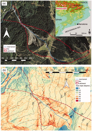
From a geological point of view, the catchment is located in the Axial Pyrenees, where bedrock is formed of Palaeozoic metamorphic rocks including slates and phyllites (Muñoz 1992). An irregular layer of colluvium and glacial deposits cover the bedrock. The most important morphologic feature is the large open scarp in the middle area of the catchment, where the lateral moraine is covering the bedrock with an important thickness. The scarp covers an area of about 0.09 km² between 1425 and 1710 m a.s.l. and has slope angles between 30° and 70° (Figure 1b). The relief in this area is very irregular due to the presence of large blocks in the moraine and badland- like morphology with deep gullies.

Different types of slope mass-wasting processes in the lateral moraine have formed the large scarp since the last glaciation. Nowadays, the most important torrential processes, which affect the morphology of the scarp, are debris flows and rockfalls (Hürlimann et al. 2012, 2014). They start in the steep scarp, move down slope and mostly stop on the fan. The activity of the torrential processes is high, as 10 debris flows and 24 debris floods have been detected by a monitoring system installed in the catchment, since 2009. The monitoring system is equipped with a wide variety of in situ sensors connected wired and wirelessly, providing data on triggering conditions and post-failure behaviour of torrential processes (Hürlimann et al. 2014). Thus, the Rebaixader catchment is a perfect site to apply and compare different geomatic techniques for the analysis of morphologic changes.

3. Data and methods

In this study, four different geomatic techniques were applied for the capture of the ground data: i) digital photography of historic aerial photographs between 1946 and 1992 (DP-HAP), ii) airborne LiDAR scanning (ALS), iii) terrestrial LiDAR scanning (TLS); and, iv) digital photography from UAV (DP-UAV) (Table 1).

Table 1. Date of data capture and applied techniques of the different Digital Elevation Models (DEM).

Date (month year)	Technique applied	Abbreviation of resulting DEM
February 1946	Photogrammetry	DP-HAP1946
August 1957	Photogrammetry	DP-HAP1957
July 1975	Photogrammetry	DP-HAP1975
August 1992	Photogrammetry	DP-HAP1992
October 2011	ALS	ALS2011
May 2012	TLS	TLS2012
July 2014	TLS	TLS2014
September 2015	TLS	TLS2015
June 2016	Photogrammetry	DP-UAV2016

3.1. Digital photogrammetry

3.1.1. Digital photogrammetry with air photographs

A total of four 3d models were built with historic aerial photographs (Table 2). The format of all them was 23 × 23 cm.

Table 2. Characteristics of the historic aerial photographs (AMS stands for Army Map Service).

Abbreviation	Source	Number of photos used	Pixel (μm)	Height above terrain (m)	Focal length (mm)	Approximate scale
DP-HAP1946	AMS (Set A)	12	21	5600	∼150	1:40,000
DP-HAP1957	AMS (Set B)	2	21	4000	151.36	1:30,000
DP-HAP1975	ICGC	3	15	3100	152.96	1:20,000
DP-HAP1992	ICGC	3	14	3980	152.12	1:22,000

The first 3D model, DP-HAP1946, was obtained from the photographs of the first American flight over Spain, which is also called ‘set A’ flight. This survey was carried out by the US Army during February 1945 and October 1946. The photographic cameras utilized during this campaign were Fairchild K-17B y K18 with wide-angle lenses producing high distortions. The resulting photograms did not include neither fiducial marks nor metrics, which are necessary to achieve classic cartographic products (Pérez et al. 2014). The final model was created by 12 photographs, whose negatives were scanned at a resolution of 1210 dpi. So, the ground resolution (equivalent to GSD, Ground Sampling Distance) was 0.73 m. Subsequently, the software Agisoft PhotoScan (Agisoft 2018) was used, since it allows the handling of photographs taken with non-metric cameras and approximated internal orientation parameters. We used five control points, which were clearly identified on the photograms and on the present cartography. PhotoScan software generated the model automatically by linking points using SIFT algorithms (de Matías et al. 2009; Chen et al. 2017). Finally, a dense point cloud of the zone of interest with 0.5 points/m² was obtained.

The second model DP-HAP1957, which is called ‘set B’ flight because it was the second American flight. It was carried out between 1956 and 1957. This flight used photographic cameras Fairchild T-11 with Metrogon lens and controlled distortion. They included fiducial marks and used metric cameras (Pérez et al. 2014). The photogrammetric adjustment of the block was created using 4 photographs, whose negatives were scanned at a resolution of 1210 dpi. So, the equivalent GSD was 0.63 m. The photogrammetric adjustment was performed with 6 ground control points. A dense point cloud with 0.5 points/m² was obtained.

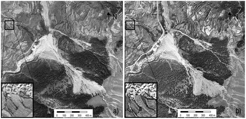
A comparison of the orthophotographs obtained from the two oldest flights (1946 and 1957) is shown in Figure 2, which reflects the better quality of the 1957 flight.

Figure 2. Orthophotographs of the study area obtained from flight 1946 (a) and 1957 (b).

The third model, DP-HAP1975, was realized by the private company Aerofoto, S.A. (AFSA) during July 1975. The photographic cameras utilized during this survey were Wild RC10 with wide-angle lenses and focal length of 152.96 mm. The photogrammetric block was generated by three photographs and the scan resolution was 1690 dpi, and the equivalent GSD was 0.30 m. The photogrammetric adjustment was performed with 68 tie points and 7 control points. A dense point cloud of the zone of interest was obtained with a resolution of 0.5 points/m².

The forth model, DP-HAP1992, was performed by ICGC. The photographic camera used during this survey was Wild RC10 with wide-angle lenses and focal length of 152.12 mm. The photogrammetric model was calculated incorporating three photographs, which were scanned at 1814 dpi (the equivalent GSD was 36 cm). Afterwards, the model was created with 5 ground control points. A dense point cloud of the zone of interest was obtained with 2 points/m².

For all the point clouds obtained from photogrammetry, vegetation has been removed in the study area, when dense forest was observed in the orthophotographs. In contrast, areas of shrubs and grass were not filtered inside the scarp, since this task is too time-consuming and cost-benefit is not justified. To compare the different models a mask was used in the small areas, where trees were observed.

3.1.2. Digital photogrammetry using UAV

The UAV applied in this study was a quadcopter DJI Inspire 1 Pro 4 K with GPS and Zenmuse X5 with a photographic camera DJI FC550, which has a focal length of 15 mm, a 4/3 CMOS sensor with a resolution of 16 Mpx (4608 × 3456, RGB), 17.50 mm × 13.125 mm frame and a resulting pixel size of 3.76 µm.

The UAV survey in July 2017 was performed at about 100 m above the terrain surface and produced images with a GSD lower than 10 cm. The photographs were taken vertically and obliquely depending on the inclination of the ground of the corresponding study zone. 1021 out of the 1500 initial photographs were selected for the block adjustment and the subsequent creation of the model. In this case, 72,000 tie points and 9 ground control points were used in order to permit an excellent adjustment. The targets have dimensions of 20 cm × 20 cm, with 2 × 2 checked boards. Their coordinates were obtained from the bases of the topographic network previously mentioned using a laser total station. The absolute accuracy in these coordinates are better than 3 cm for the planimetric ones and 4 cm in the altitude. The point cloud has a density of 85 point/m².

3.2. Laser scanning

3.2.1. Terrestrial laser scanning

Four surveys were carried out during May 2012 and September 2015 applying two different sensors. During the first field campaign, we used a Leica HDS880 with a nominal scan distance up to 1400 m (for bedrock surfaces), and a precision of 20 mm at 1000 m and 0.01° angular. The georeferencing of this sensor is direct due to it is able to set in a known point and oriented.

The May 2012 survey was performed from 8 base stations, from E1 to E8 in Figure 3, in order to cover the entire study area. However, the complex morphology, which caused many parts of the area out of the line of sight, and the minor reflectivity of the surface, resulted in multiple small zones without of data. These zones are mostly located at the higher part of the open scarp, where the erosion formed large rills in the glacial deposit and consequently a very heterogeneous ground surface. Such morphologic characteristics, humidity at the surface and long distance scanning strongly impended a correct data capturing, a fact that was already described in other studies (Fey and Wichmann 2017). The filtering and registration of the different point clouds was performed in three steps: First, the noise, which was mainly caused by fog and rainfall during the survey, was deleted. Second, the vegetation was filtered and deleted using the differences in the reflectivity. These two steps were carried out manually. Third, the point clouds were merged applying the Cyclone of Leica. The point cloud had an average resolution of 20 cm.

Figure 3. GPS network established in the area to obtain coordinates of the targets and ground control points.

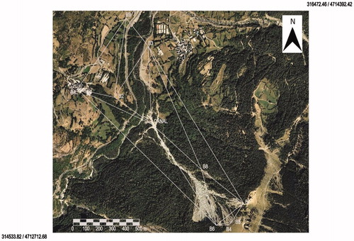
The following three TLS campaigns between October 2012 and September 2015 were performed by a RIEGL LPM321 with a nominal scan distance of 6000 m, and a precision of 25 mm at 50 m and 0.009° angular. The surveys were carried out at 5 base stations (three of them were the same as in the first TLS campaign) and the georeferencing was achieved due to the reflector targets situated at known coordinates. Finally, we applied the well-known Iterative Closest Point (ICP) algorithm for the registration of the point clouds (Besl and McKay 1992; Chen and Medioni 1991; Zhang 1994; Gruen and Akca 2005). This algorithm is implemented in the RIEGL software RISCAN PRO (Riegl 2018) and was used in this study for the merging of the point clouds of each single TLS survey. A multi-temporal use of the algorithm was avoided because of the possible morphologic changes in the study site. The scanning of stables zones in the neighborhood was not taken into account due to the difficult environment. Like in the previous case, the resulting point cloud had a resolution of 20 cm, although there were some areas without of data.

3.2.1. Airborne laser scanning

Airborne Laser Scanning (ALS) is mostly applied for regional surveys and the resulting density of the point cloud is principally related to the flight altitude (in general, 0.5–2 points/m²). GNSS and differential GNSS techniques provide a correct georeferencing of the point clouds.

In this study, the ICGC offered a raster file of terrain surface with a cell size of 2 m. This DEM was achieved by an Optech ALTM 3025 sensor mounted on an airplane. The point density was 0.5 points/m² and the RMSE (Root Mean Square Error) of the metadata about 0.15 m. However, RMSE-height values strongly vary depending on the slope angle (Moreno Baños et al. 2011) and may reach 0.7 m for slope angles between 40 and 50° or even 1.3 m for 50–60°.

3.3. Georeference system

A fundamental aspect for the comparison of the different terrain models is the georeference, which must be the same for all of them. In this study, all the models are represented in UTM 31 N (ETRS89). Regarding altitudes, the geoid model EGM08D595 was applied to transform the ellipsoidal heights into orthometric values. This model is the result of the adjustment of the EGM08 global model to Catalonia. Its altitude error in our test area is neglected for the purpose in this study.

The DEM’s derived from TLS and DP-UAV were georeferenced using ground control points measured from the 9 bases of the local topographic network established by GNSS observations, Figure 3. This network has been computed incorporating permanent station of the Cartographic and Geological Institute of Catalonia (ICGC) network. The accuracy of the coordinates of bases is better than 2 cm in planimetric coordinates and 3.2 cm in altitude. In contrast, the four models obtained by DP of historic aerial photographs were georeferenced by control points that were selected on the official topographic maps with a scale of 1:5000 available at the ICGC (www.icgc.cat). The accuracy for this coordinates, according with the ICGC’s technical specifications is of 1 m for the planimetric coordinates and 1.5 m for the altitude. This accuracy will condition the accuracy of the DP-HAP models, since in any case could be better than these values.

Finally, the ALS model, which was elaborated by the ICGC, is in the planimetric reference system ED50 and uses the geoid model UB91 for altitudes. Therefore, the transformation of this initial ALS model was necessary for both planimetric coordinates and altitudes in order to achieve a model with the same reference systems as the other ones. The transformation was carried out using the parameters established by the ICGC. In this case a 2D similarity , Equations (1) and (2), is enough for the planimetric coordinates. (1) $${\mathit{x}}^{\mathrm{\prime }}=\lambda \mathit{x}\text{cos}\mathit{\alpha }-\lambda \mathit{y}\text{sin}\mathit{\alpha }+{\mathit{T}}_{\mathit{x}}$$(1)

(2) $$\mathit{y}\mathrm{\prime }=\lambda \mathit{y}\text{cos}\mathit{\alpha }+\lambda \mathit{x}\text{sin}\mathit{\alpha }+{\mathit{T}}_{\mathit{y}}$$(2)

where λ is the scale factor, α the rotation between systems and T_x, T_y translations. The maximum residual obtained in this case was of 0.021 m and the minimum of 0.007 m.

In the case of altimetry, the difference between both models (UB91-modified and EGM08D595) in 7 points that were used for testing is approximately 3 cm; less than the error of the models. Therefore, it will not be necessary to apply a vertical offset.

3.4. Uncertainty analysis

Ground control points were defined inside the study area in order to carry out a quantitative accuracy assessment of all the models. The Ground Control Points (GCP) were selected in places close to the zone affected by the torrential processes, but not in a dangerous place for the in situ measurements, since we defined their coordinates by total station (Figure 4). It would be desirable that they had a homogenous distribution, but this was not possible for the reason previously mentioned. The GCPs were divided into three classes using the local slope angle as classification factor: i) smooth terrain (slope angles between 0 and 15°), ii) medium slope terrain (15°–30°) and iii) steep terrain (30°–60°). Slope angles higher than 60° were not found. Each class includes between 6 and 8 GCPs. This number is rather low, because stable zones without of vegetation are scarce, but characterizes the complex environmental conditions in our study area.

Figure 4. Location of the ground control points (GCP) used for the accuracy assessment. GCPs used for the ALS, TLS and DP-UAV models (top) and used for DP-HAP (bottom).

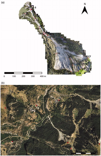
Regarding the models obtained by historic aerial photographs and DP, different GCPs were selected (Figure 4), because the ground surface and vegetation cover has changed in the past. Therefore, GCP that are situated out of the open scarp, were selected. Finally, seven GCPs were defined to check the four models obtained by DP-HAP.

The accuracy analysis was performed in two steps. First, the original point clouds were analysed and RMSE-values calculated. This task could be performed for the TLS and DP-UAV models. Regarding the DP-HAP models, it could only be performed for DP-HAP1992, since the other models have a too low resolution. Second, the raster files, which were created by the TIN-algorithm and a cell size of 2 m, were evaluated by the two following methods: a bilinear interpolation as well as the ‘point sampling tool’ plug-in of QGIS.

In order to establish the real change between the models of different years, the minimum level of detectable changes (min LoD) was used, since LoD is directly related to the model errors. Because the model differences were calculated applying the law of variance-covariance propagation, the resulting error of the model of differences was expressed as: (3) $${\sigma }_{\text{dif}}=\sqrt{{\sigma }_{\text{MDT}\_\text{new}}^2+{\sigma }_{\text{MDT}\_\text{old}}^2}$$(3)

where$\mathrm{}{\mathrm{}\sigma }_{\text{MDT}\_\text{new}}^2$ is the variance for recent model and${\mathrm{}\sigma }_{\text{MDT}\_\text{old}}^2$ is the variance for the older model.

To evaluate the significance of the uncertainties (${\sigma }_{\text{dif}})$ in predicted elevation changes among models the minimum LoD or a probabilistic thresholding can be used (Wheaton et al. 2010). In our case, since a spatial variability is important, we have used the last one (Brasington et al. 2003; Victoriano et al. 2018) to discard noise and consider only real changes. To establish the threshold to consider a change statistically significant or not, Student's t-distribution was applied, calculating the t-parameter for each cell of the resulting difference model by (4) $$t=\frac{\left|\Delta Z\right|}{{\sigma }_{\text{dif}}}$$(4)

$\Delta Z$ corresponds to the elevation differences in this cell of the models of different years. The probability (p) of a realistic elevation difference was achieved by the value of t. In this study, a reliability of 68%, which coincides with a standard deviation, was defined to assume no elevation change for cells with p < 0.32.

3.5. From point cloud to raster DEM

The most common procedure in the comparison of multi-temporal terrain models is transformed them into raster DEM for easy handling. However, the accuracy of the DEM is not only depending on the geomatic technique applied during the data capturing, but also on the selected interpolation method to transform the point cloud into a raster DEM (Ashraf et al. 2017).

The most common interpolation methods are: Triangulation Irregular Network, Inverse Distance Weighted, Natural Neighbour, Kriging, Splines and methods based on Radial Basis Functions (RBF) (Ali 2004; Aguilar et al. 2005; Hejmanowska 2007; Goff and Nordfjord 2008; Hejmanowska 2007; Ashraf et al. 2017). Among all of them, the Triangulation Irregular Network (TIN) interpolation is widely used because of its simplicity and its ability to resolve abrupt changes in topography. Since the data provided by TLS and digital photogrammetry are dense we will use this method in the following sections.

It is important to always apply the same method since the use of one or other method provide different results (Li and Heap 2008; Ashraf et al. 2017).

4. Results and discussion

The results of three different aspects are presented and discussed herein: i) the distinct accuracies of point cloud and raster models, and ii) the influence of the different techniques on the resulting volume quantification between two models, and iii) the erosion rate over the last 70 years in the study area.

4.1. Accuracy assessment of digitals models

In this section we analyze the quality of the models in a double way. First, we determine the accuracy of the DP-HAP and DP-UAV models regarding the photogrammetric adjustment. Then, we use some selected ground control points to evaluate the quality of the models.

The quality of the models achieved by digital photogrammetry clearly shows the difference between the models that were created from historic aerial photographs and the one generated by photos taken by the UAV. This can be easily explained, since the accuracy of the final model depends mainly on the quality of the control points used in the block adjustment, the number of photograms available and the overlap among the different images. For the adjustment of Historical Photographs points obtained from the existing cartographic maps are used and their precision is around 1 m. After the photogrammetric process, the altimetric errors of the models obtained by historic photographs exceed 0.65 m. The best accuracy is reached in the DP-HAP1975 (0.56 m) and the worst in the DP-HAP1946 (0.95 m). The accuracies of DP-HAP1992 and DP-HAP1956 were 0.74 m and 0.62 m, respectively. It has to be kept in mind that three of the four DP-HAP models were created by only two or three photograms (Table 1). In contrast, the adjustment of the photogrammetric block from UAV included a total of images and has an accuracy of 0.15 m. During the data capturing of the TLS-models, an accuracy of 0.15 to 0.30 m was achieved. This value is estimated, since the error of the model does not have a homogeneous distribution and may vary between the central parts and the surfaces located in the direction of maximum slope angles. The elimination of the errors during TLS-surveys is very complex, especially when working at large distances and stable sub-areas instead of fixed targets are used for the control (Fey and Wichmann 2017). In our case, the collocation of targets was very difficult due to the dangerous natural processes in many parts of the zone, the dense vegetation in the adjacent parts and the complex morphology with large slope angles, rills and big blocks.

Finally, the accuracy of the ALS-model is given by the characteristics of the raster-file that was directly obtained from ICGC. The technical specifications of this model remark a vertical error of 0.15 m in smooth flat areas and 0.90 m in inclined zones. In very steep mountain areas, like our test site, vertical errors of up to 1.30 m can occur (Moreno Baños et al. 2011).

The results of all the nine models show that the accuracy has strongly improved when comparing the historic DP-HAP models (Table 3) with the more recent models obtained by ALS, TLS or DP-UAV (Table 4). RMSE-values are high for DP-HAP models, because the goal of these photogrammetric flights focused on cartographic aspects at medium scale and not on the creation of high resolution DEMs. Another general outcome is that the errors are higher for the raster files than for the point cloud.

Table 3. RMSE-values, units in meters, of the DP-HAP models using ground control points obtained from cartography (see Fig. 4 for location of GCPs).

	1946 DP-HAP	1957 DP-HAP	1975 DP-HAP	1992 DP-HAP
Point Cloud	1.72	1.41	0.85	1.63
2×2 raster bilinear	1.92	1.57	0.94	1.77
2×2 raster (QGIS)	1.98	1.65	1.02	1.84

Table 4. RMSE-values, units in meters, of the ALS, TLS and DP-UAV models using ground control points obtained by total station measurements (see Figure 4 for location of GCPs).

	Slope class	2011 ALS	2012.1 TLS	2014 TLS	2015 TLS	2016 DP-UAV
Point Cloud	0°–15° 15°–30° 30°–60°	ND ND ND	0.56 0.60 0.68	0.65 0.69 0.82	0.45 0.59 0.78	0.21 0.27 0.17
2×2 raster bilinear	0°–15° 15°–30° 30°–60°	0.22 0.58 0.84	0.55 0.69 0.98	0.77 0.65 1.12	0.30 0.63 0.90	0.29 0.55 0.66
2×2 raster (QGIS)	0°–15° 15°–30° 30°–60°	0.29 0.52 0.79	0.75 0.79 1.12	0.88 0.71 0.90	0.17 0.53 0.93	0.25 0.51 0.77

The RMSE-value from the height differences was obtained for each slope class.

Analyzing the most recent models in details, we detected that, the errors are larger in steep terrains. This trend was already observed in other studies (Moreno Baños et al. 2011).

4.2. Uncertainty due to raster resolution on the quantification of ground movement

The selection of the most adequate cell size of the involved raster files is fundamental. In the following, we compare raster files with two different cell sizes (0.5 and 2.0 m) and perform a detailed analysis for three test zones located in our basin (Figure 7). Two test zones are located in the middle part of the open scarp and each of them covers 2500 m² (50 per 50 m). The third one is situated at the upper bound of the scarp, where the morphology is more complex, and covers 625 m² (25 per 25 m, see Figure 7).

The TLS2012 model and the DP-UAV2016 model were selected for the comparison, because both models present a good accuracy and a dense point cloud. This was necessary, since the point clouds were used as reference model.

The quantification of volume differences normally neglects the small topographic changes. The standard deviation of the TLS model regarding the elevation is 0.22 m and 0.15 m for the UAV-model. Applying the variance propagation Equation (3)(3) $${\sigma }_{\text{dif}}=\sqrt{{\sigma }_{\text{MDT}\_\text{new}}^2+{\sigma }_{\text{MDT}\_\text{old}}^2}$$(3) differences larger than ±0.26 m are not included in the calculations. The distance between the two point clouds was calculated applying the M3C2 distance algorithm in “CloudCompare” (Lague et al. 2013). Detailed results of the DoD (Difference of Distance) are shown in Figure 5 for the zones 1 and 3. In addition, the raster files were compared by an own software developed in MATLAB to obtain the quantification of total accumulation and erosion in the three test zones.

Figure 5. DEM of Difference (DoD) between model TLS2012.1 and DP-UAV2016. (a) Situation of the three test zones and corresponding DoD. (b) Detailed results of the DoD of zone 1 and zone 3.

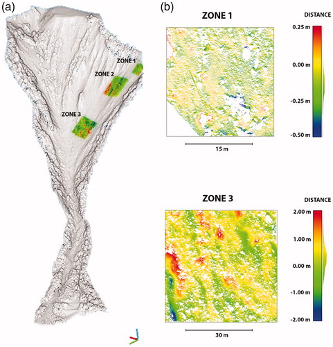
The volumes of all these calculations are shown in Figure 6 and demonstrate that the influence of the cell size is not significant. Surprising is also the fact that the calculations with point clouds revealed no clear improvement. The results indicate that the values of erosion and accumulations are smallest in the 0.50 m raster and highest in the 2 m raster. From a geomorphological point of view, the results show that the principal process is erosion in the higher parts of the scarp (zone 1 and 2), where slopes are steeper. In contrast, accumulation is the main morphologic process in zone 3, which is located in the lower part of the scarp. Largest distances between the topographic models of 2012 and 2016 are observed due to the failure of big blocks and other mass-wasting processes. Such differences are visible, since some mobilized blocks have diameters up to 1 or 3 m (Figure 5).

Figure 6. Total erosion (a) and accumulation (b) calculated by three different methods (DoD of point clouds, 0.5 m and 2.0 m raster) in the three test zones between TLS2012.1 and DP-UAV2016.

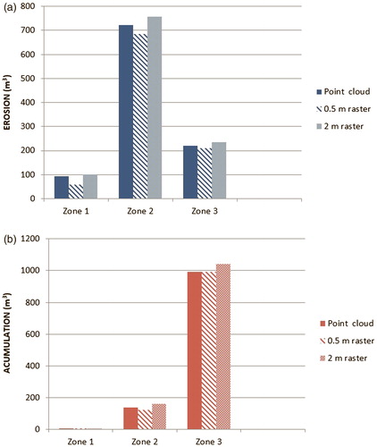
At last, even in our case with a very heterogeneous morphology, the differences of the volume calculations obtained by the different methods are not important. Thus, an analysis with a 2 m raster file would be adequate. A more detailed and precise analysis of this topic is only possible, if both models were created by DP-UAV. Then, not only DoDs can be generated, but also a raster of distribution errors, which enables the application of Equation (3)(3) $${\sigma }_{\text{dif}}=\sqrt{{\sigma }_{\text{MDT}\_\text{new}}^2+{\sigma }_{\text{MDT}\_\text{old}}^2}$$(3) to each cell and the detection of significant differences.

4.3. Temporal evolution of erosion

As a final task, the erosion rate in the Rebaixader scarp was calculated over a time span of 70 years (1946–2016). This task is rather complex, because the area with active erosion has been variable over time. On one side, the total area of the open scarp has increased due to erosion at its lateral limits and backward displacement of the head scarp at the top. On the other side, vegetation cover has changed during the last 70 years with an increase of grass, shrubs and trees in the Eastern part of the scarp and at its lower part, near the channelized area (compare ortophotographs of 1946 and 1957 in Figure 3 with the one of 2016 in Figure 4).

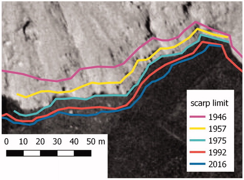
In a first step, the temporal evolution of the erosion was estimated in a qualitative and visual manner comparing the retreat of the upper limit of the open scarp, which is visible in the different orthophotographs (Figure 7). An exact quantification of backward displacement of the scarp is difficult, but the following general patterns can be observed: the largest retreat rates occurred during the first 11 years (1946–1957) and in diminishing importance until 1975 or 1992. In contrast, minor retreat rates are detected during the last 23 years (1992–2016). This reduction of the retreat rate over the studied time span is also supported and maybe correlated with the increase of vegetation cover in the down slope scarp area.

Figure 7. Position of the upper limit of the open scarp between 1946 and 2016. The 1975 orthophotograph is shown as background.

In the second step, the nine available DEMs were taken into account to quantify the erosion rates. Finally, the three TLS-models must be rejected, since they did not cover the entire test area. Therefore, the calculations included six DEMs: four DP-HAP models (1946–1992), the ALS2011 model and the DP-UAV2016 model. The DoDs were calculated using 2 m raster files and applying standard commands of QGIS. The differences among the models 1946–1957, 1957–1975, 1975–1992, 1992–2011, 2011–2016 have been obtained. The thresholds of significant change in these differences were calculated by using the values that were achieved from Equations (3)(3) $${\sigma }_{\text{dif}}=\sqrt{{\sigma }_{\text{MDT}\_\text{new}}^2+{\sigma }_{\text{MDT}\_\text{old}}^2}$$(3) and (4)(4) $$t=\frac{\left|\Delta Z\right|}{{\sigma }_{\text{dif}}}$$(4) . In this process the values of RMSE from Tables 3 and 4 have been considered. Since we do not have neither the information of all the slope ranges nor all the point clouds, the values from the bilinear interpolation and the slope range 15°–30° were used. Therefore, for instance, the threshold for the difference of the 1946–1957 models was 1.38 m, while it was 0.38 m in the case of the 2011–2016 models. Changes on the open scarp area were considered by the calculation of the erosion rate. First, a polygon representing the open scarp area was drawn for each of the selected years, using the corresponding ortophotograph. These polygons contain zones without grass, shrubs or trees. DEMs of open scarp areas were extracted from original DEMs, using these polygons as masks, therefore the analysis only included area without vegetation. By doing so, possible erosion errors associated to the increase of vegetation or shrubs were avoided. Finally, the annual erosion rate was computed using the polygon area and the time span between the two raster files.

Within the studied period, maximum open scarp area was identified in 1957, corresponding to the end of the time period with maximum annual erosion (Figure 8a). After 1957, the increase of vegetation in the Eastern and lower parts of the head scarp supposed a reduction of the total open scarp area, as well as lower annual erosion volumes and annual erosion rates (Figure 8b).

Figure 8. Temporal evolution of annual erosion rate in the Rebaixader site between 1946 and 2016. (a) Annual erosion and area of the open scarp. (b) Annual erosion rate (dashed line indicates the average value).

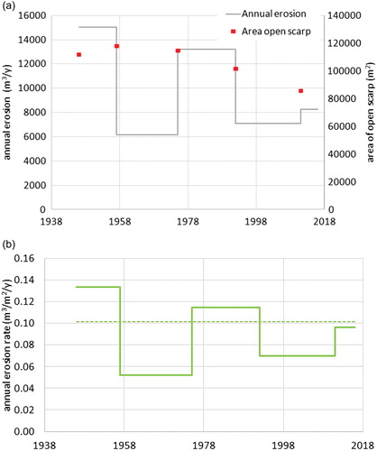
The results show that the average annual erosion rate in the Rebaixader scarp was of 0.09 m³/m²/y, which coincides rather well with other studies performed in torrential catchments [e.g. (Bennett et al. 2012)]. The temporal evolution of the erosion rate reveals that, after the initial period (1946–1957) with major erosion rate, the mean value of annual erosion rate was 0.08, with higher values between 1975 and 1992. Other time intervals have similar values. The maximum erosion in the initial period of this study could be associated with historical floods and landslide episodes occurred during the 1930’s and 1940’s in the Pyrenees (e.g. Hürlimann et al. 2003; Portilla et al. 2010). Torrential processes and landslides have probably also occurred in the Rebaixader catchment by the same rainfall episodes that also caused the floods, leaving more open area exposed for erosion. This hypothesis is supported by the observation of a great number of open scarps in the ortophotographs not only in the Rebaixader catchment, but all over the territory nearby. The second period with large erosion (1975–1992) may be related to the exceptional and catastrophic 1982 flood episode, which affected large parts of the Pyrenees and created hundreds of landslides and torrential flows [e.g. (Corominas and Alonso 1990)]. Unfortunately, a clear evidence of an important torrential process in the Rebaixader catchment during the 1982 flood has not yet been found. Maybe, because our test catchment does not include any infrastructure that could have been damaged.

5. Conclusions

The detection of morphologic changes in high mountain environments is an important task for the correct understanding of geomorphologic processes and their impact. In this study, we focused on the monitoring of erosion and accumulation associated with torrential mass wasting in a large open scarp. We compared four geomatic techniques and evaluated the quality of nine resulting digital elevation models. Finally, DEMs from 1946 (created by the oldest aerial photograph available) till 2016 (most recent UAV flight) were generated, and therefore allowed an analysis of changes over an observation time span of 70 years.

As a general conclusion, we can state that two typical features of high mountain environments complicated our monitoring surveys: the vegetation and the complex relief. Both features strongly limited the usefulness of applying TLS, because many parts of the area under consideration were not in the line of sight. The morphologic characteristics of the open scarp (large blocks, large gullies and steep slopes) increased difficulties especially for TLS application, but also for the other techniques. Only DP-UAV resolved these constraints by taking photographs perpendicular to the slope surface inclining the camera. Regarding the presence of vegetation, we had to filter the vegetated areas manually, since a correct definition was not possible using automatized procedures. Another drawback of monitoring mountainous regions with multiples morphological active processes is the fact that the selection of stable control points is very difficult, especially when surveying many decades.

In addition, the following specific conclusions can be expressed: i) The comparison of the different techniques showed that the most precise DEMs were achieved by applying DP-UAV and ALS. However, cost-benefit ratio of DP-UAV technique is much better than of ALS. ii) The historic aerial photographs, which have been taken for cartographic purposes, only allow the creation of DEMs with limited accuracy. Thus, the detection of small morphologic changes is impossible and only large differences in altitude can be determined. iii) The comparison of DoDs obtained from initial point clouds and both 0.5 m and 2.0 m raster files indicated that differences in our test area are small.

Summarizing, we recommend the application of DP-UAV for monitoring active morphologic processes in complex high mountain terrains like torrential basins. When historic topographic changes have to be detected, the application of DP to the available aerial photographs is necessary, but results strongly depends on the quality of the photos. In our case, the error of the resulting DEMs was rather large, since the historic aerial photographs have been taken for cartographic purposes. Nevertheless, the rate of slope mass-wasting, which was determined over the time-span of the last 70 years, coincides well with values obtained in other areas.

Acknowledgements

We also thanks Ignacio López and Jesús Revuelto of the Pyrenean Institute of Ecology, Spain and Roger Ruiz of UPC BarcelonaTECH for their help in the data capture during TLS and UAV campaigns.

Additional information

Funding

This study was supported by the research projects “Slope mass-wasting under climate change. Physical mechanisms, predictive modelling and possible mitigation strategies.” (SMuCPhy Ref. BIA2015-67500-R) and “Characterization and modeling of rockfalls" (RockModels. Ref. BIA2016-75668-P, AEI/FEDER, UE) funded by the Spanish Ministry of Economy and Competitiveness.

References

- Agisoft. 2018. No Title. Agisoft. [cited 2018 Jan 1]. www.agisoft.com
- Aguilar FJ, Agüera F, Aguilar MA, Carvajal F. 2005. Effects of Terrain morphology, sampling density, and interpolation methods on grid DEM accuracy. Photogramm Eng Remote Sens. 71(7):805–816. http://essential.metapress.com/openurl.asp?genre=article&id=doi:10.14358/PERS.71.7.805%5Cn; http://openurl.ingenta.com/content/xref?genre=article&issn=0099-1112&volume=71&issue=7&spage=805
- Aguilar MA, Aguilar FJ, Fernández I, Mills JP. 2013. Accuracy Assessment of Commercial Self-Calibrating Bundle Adjustment Routines Applied to Archival Aerial Photography. Photogram Rec. 28(141):96–114.
- Aicardi I, Dabove P, Lingua AM, Piras M. 2017. Integration between TLS and UAV photogrammetry techniques for forestry applications. iForest. 10(1):41–47.
- Aitkenhead MJ, Dalgetty IA, Mullins CE, McDonald AJS, Strachan NJC. 2003. Weed and crop discrimination using image analysis and artificial intelligence methods. Comput Electron Agric. 39(3):157–171.
- Ali TA. 2004. On the selection of an interpolation method for creating a Terrain Model (TM) from LIDAR data. In: Proc Am Congr Surv Mapp Conf 2004. Nashville; 1–18.
- Ashraf I, Hur S, Park Y. 2017. An investigation of interpolation techniques to generate 2D intensity image from LIDAR data. IEEE Access. 5:8250–8260.
- Barilotti A, Sepic F, Abramo E. 2008. Automatic detection of dominated vegetation under canopy using Airborne Laser Scanning data. In: Proc SilviLaser. Edinburgh:134–143.
- Bennett GL, Molnar P, Eisenbeiss H, Mcardell BW. 2012. Erosional power in the Swiss Alps: Characterization of slope failure in the Illgraben. Earth Surf Process Landforms. 37(15):1627–1640.
- Besl P, McKay N. 1992. A method for registration of 3-D shapes. IEEE Trans Pattern Anal Mach Intell. 14(2):239–256.
- Blasone G, Cavalli M, Marchi L, Cazorzi F. 2014. Monitoring sediment source areas in a debris-flow catchment using terrestrial laser scanning. Catena. 123:23–36. Available from: http://dx.doi.org/10.1016/j.catena.2014.07.001
- Bossi G, Cavalli M, Crema S, Frigerio S, Quan Luna B, Mantovani M, Marcato G, Schenato L, Pasuto A. 2015. Multi-temporal LiDAR-DTMs as a tool for modelling a complex landslide: A case study in the Rotolon catchment (eastern Italian Alps). Nat Hazards Earth Syst Sci. 15(4):715–722.
- Brasington J, Langham J, Rumsby B. 2003. Methodological sensitivity of morphometric estimates of coarse fluvial sediment transport. Geomorphology. 53(3–4):299–316.
- Bremer M, Sass O. 2012. Combining airborne and terrestrial laser scanning for quantifying erosion and deposition by a debris flow event. Geomorphology. 138(1):49–60. Available from: http://dx.doi.org/10.1016/j.geomorph.2011.08.024
- Cardenal J, Delgado J, Mata E, González A, Olague I. 2006. Use of historical flight for landslide monitoring. Spatial-AccuracyOrg. 129–138. http://www.spatial-accuracy.org/system/files/Cardenal2006accuracy.pdf
- Cavalli M, Goldin B, Comiti F, Brardinoni F, Marchi L. 2017. Assessment of erosion and deposition in steep mountain basins by differencing sequential digital terrain models. Geomorphology. 291:4–16.
- Chen T, Ren L, Yuan F, Yang X, Jiang S, Tang T, Liu Y, Zhao C, Zhang L. 2017. Comparison of Spatial Interpolation Schemes for Rainfall Data and Application in Hydrological Modeling. Water. 9(5):342. http://www.mdpi.com/2073-4441/9/5/342
- Chen Y, Medioni G. 1991. Object Medeling by Registration os Multiple Range Images. In: IEEE Int Conf Robot Autom. Sacramento: IEEE international Conference on Robotics and Automation; 2724–2729.
- Corominas J, Alonso E. 1990. Geomorphological effects of extreme floods (November 1982) in the southern Pyrenees. In: Proc Hydrol Mt Reg Reserv Water Slopes. Lausanne: IAHS; 295–302.
- Eisenbeiss H, Lambers K, Sauerbier M. 2005. Photogrammetric recording of the archaeological site of Pinchango Alto (Palpa, Peru) using a mini helicopter (UAV). In: Figueiredo A, editor. Annu Conf Comput Appl Quant Methods Archaeol CAA. Toma; 21–24. http://www.photogrammetry.ethz.ch/general/persons/karsten/paper/eisenbeiss_et_al_2007.pdf
- Faugeras O, Luong Q-T. 2001. The geometry of multiple images. 2nd ed. Cambridge: MIT Press.
- Fey C, Wichmann V. 2017. Long-range terrestrial laser scanning for geomorphological change detection in alpine terrain – handling uncertainties. Earth Surf Process Landforms. 42(5):789–802.
- Gée C, Bossu J, Jones G, Truchetet F. 2008. Crop/weed discrimination in perspective agronomic images. Comput Electron Agric. 60(1):49–59.
- Goff JA, Nordfjord S. 2008. Interpolation of fluvial morphology using channel-oriented coordinate transformation: A case study from the New Jersey shelf. Math Geol. 36(6):643–658.
- Gonçalves-Seco FJ, Miranda D, Crecente R FJ. 2006. Digital terrain model generation using airborne LiDAR in a forested area Galicia, Spain. In: Proc 7th Int Symp Spat accuracy Assess Nat Resour Environ Sci. Lisboa; 169–180.
- Gruen A, Akca D. 2005. Least squares 3D surface and curve matching. ISPRS J Photogramm Remote Sens. 59(3):151–174.
- Guijarro M, Pajares G. 2009. On combining classifiers through a fuzzy multicriteria decision making approach: Applied to natural textured images. Expert Syst Appl [Internet]. 36(3):7262–7269. http://dx.doi.org/10.1016/j.eswa.2008.09.021
- Hejmanowska B. 2007. Analysis of NMT in the form of GRID and TIN on example of data from OKI. Archives of Photogrammetry. Cartogr Remote Sens. 17281–289.
- Hürlimann M, Corominas J, Moya J, Copons R. 2003. Debris-flows events in the Eastern Pyrenees, Spain. Preliminar study on initiation and propagation. 3rd Int. Conf. on Debris-Flow Hazards Mitigation, Davos, Switzerland, 115–126.
- Hürlimann M, Abancó C, Moya J. 2012. Rockfalls detached from a lateral moraine during spring season. 2010 and 2011 events observed at the Rebaixader debris-flow monitoring site (Central Pyrenees, Spain). Landslides. 9(3):385–393.
- Hürlimann M, Abancó C, Moya J, Vilajosana I. 2014. Results and experiences gathered at the Rebaixader debris-flow monitoring site, Central Pyrenees, Spain. Landslides. 11(6):939–953.
- Jaboyedoff M, Oppikofer T, Abellán A, Derron MH, Loye A, Metzger R, Pedrazzini A. 2012. Use of LIDAR in landslide investigations: A review. Nat Hazards. 61(1):5–28.
- James LA, Hodgson ME, Ghoshal S, Latiolais MM. 2012. Geomorphic change detection using historic maps and DEM differencing: the temporal dimension of geospatial analysis. Geomorphology. 137(1):181–198.
- Kamps MT, Bouten W, Seijmonsbergen AC. 2017. LiDAR and orthophoto synergy to optimize object-based landscape change: Analysis of an active landslide. Remote Sens. (8):805. 9
- Lague D, Brodu N, Leroux J. 2013. Accurate 3D comparison of complex topography with terrestrial laser scanner: Application to the Rangitikei canyon (N-Z). ISPRS J Photogramm Remote Sens. 82:10–26.
- Lato MJ, Diederichs MS, Hutchinson DJ, Harrap R. 2012. Evaluating roadside rockmasses for rockfall hazards using LiDAR data: Optimizing data collection and processing protocols. Nat Hazards. 60(3):831–864.
- Lenda G, Ligas M, Lewińska P, Szafarczyk A. 2016. The use of surface interpolation methods for landslides monitoring. KSCE J Civ Eng. 20(1):188–196.
- Li J, Heap AD. 2008. A Review of Spatial Interpolation Methods for Environmental Scientists. Geoscience Australia, Record (2008) 23.
- Liberti M, Simoniello T, Carone MT, Coppola R, D'Emilio M, Macchiato M. 2009. Mapping badland areas using LANDSAT TM/ETM satellite imagery and morphological data. Geomorphology. 106(3–4):333–343. http://dx.doi.org/10.1016/j.geomorph.2008.11.012
- Liu C, Li W, Lei W, Liu L, Wu H. 2011. Architecture planning and geo-disasters assessment mapping of landslide by using airborne lidar data and UAV images. In: Int Symp Lidar Radar Mapp Technol. Nanjing; 1–7.
- de Matías J, de Sanjosé JJ, López-Nicolás G, Sagüés C, Guerrero JJ. 2009. Photogrammetric methodology for the production of Geomorphologic maps: Application to the Veleta Rock Glacier (Sierra Nevada, Granada, Spain). Remote Sens. 1(4):829–841.
- Moreno Baños I, Ruiz García A, Alavedra JMI, Figueras POI, Iglesias JP, Figueras PMI, López JT. 2011. Assessment of airborne LIDAR for snowpack depth modeling. BSGM. 63(1):95–107.
- Muñoz A. 1992. Evolution of a continental collision belt: ECORS-Pyrenees crustal balanced cross-sectionitle. In: McClay KR, editor. Thrust tectonics. London: Chapman & Hall; p. 235–246.
- Niethammer U, James MR, Rothmund S, Travelletti J, Joswig M. 2012. UAV-based remote sensing of the Super-Sauze landslide: Evaluation and results. Eng Geol [Internet]. 128:2–11. http://dx.doi.org/10.1016/j.enggeo.2011.03.012
- Pérez JA, Bascon FM, Charro MC. 2014. Photogrammetric usage of 1956-57 usaf aerial photography of Spain. Photogram Rec. 29(145):108–124.
- Piras M, Taddia G, Forno MG, Gattiglio M, Aicardi I, Dabove P, Russo SL, Lingua A. 2017. Detailed geological mapping in mountain areas using an unmanned aerial vehicle: application to the Rodoretto Valley, NW Italian Alps. Geomatics Nat Hazards Risk. 8(1):137–149. https://doi.org/10.1080/19475705.2016.1225228
- Portilla M, Chevalier G, Hürlimann M. 2010. Description and analysis of major mass movements occurred during 2008 in the Eastern Pyrenees. Nat Hazards Earth Syst Sci. 10(7):1635–1645.
- Prokop A, Panholzer H. 2009. Assessing the capability of terrestrial laser scanning for monitoring slow moving landslides. Nat Hazards Earth Syst Sci. 9(6):1921–1928.
- RIEGL. 2018. Operating and Processing Software RiScan Pro. RIEGL LMS. Oper Process Softw RiScan Pro RIEGL LMS. Available from: www.riegl.com
- Sanjosé-Blasco JJ, Atkinson-Gordo ADJ, Salvador-Franch F, Gómez-Ortiz A. 2007. Application of geomatic techniques to monitoring of the dynamics and to mapping of the Veleta rock glacier (Sierra Nevada, Spain). Zeitschrift Geomorphol Suppl Issues. 51: 79–89. http://openurl.ingenta.com/content/xref?genre=article&issn=1864-1687&volume=51&issue=2&spage=79
- Scheidl C, Rickenmann D, Chiari M. 2008. The use of airborne LiDAR data for the analysis of debris flow events in Switzerland. Nat Hazards Earth Syst Sci. 8(5):1113–1127.
- Schürch P, Densmore AL, Rosser NJ, Lim M, Mcardell BW. 2011. Detection of surface change in complex topography using terrestrial laser scanning: Application to the Illgraben debris-flow channel. Earth Surf Process Landforms. 36(14):1847–1859.
- Stumpf A, Malet JP, Kerle N, Niethammer U, Rothmund S. 2013. Image-based mapping of surface fissures for the investigation of landslide dynamics. Geomorphology. 186:12–27. http://dx.doi.org/10.1016/j.geomorph.2012.12.010
- Tziavou O, Pytharouli S, Souter J. 2018. Unmanned Aerial Vehicle (UAV) based mapping in engineering geological surveys: Considerations for optimum results. Eng Geol. 232:12–21. https://doi.org/10.1016/j.enggeo.2017.11.004
- Victoriano A, Brasington J, Guinau M, Furdada G, Cabré M, Moysset M. 2018. Geomorphic impact and assessment of flexible barriers using multi-temporal LiDAR data: The Portainé mountain catchment (Pyrenees). Eng Geol. 237:168–180. https://doi.org/10.1016/j.enggeo.2018.02.016
- Walstra J, Chandler JH. 2004. Time for change-quantifying landslide evolution using historical aerial photographs and modern photogrammetric methods. In: Proc 20th ISPRS Congr. Istambul: ISPRS; 475–480. http://www.cartesia.org/geodoc/isprs2004/comm4/papers/395.pdf
- Wheaton JM, Brasington J, Darby SE, Sear DA. 2010. Accounting for uncertainty in DEMs from repeat topographic surveys: Improved sediment budgets. Earth Surf Process Landforms. 35:136–156.
- Zhang C, Kovacs JM. 2012. The application of small unmanned aerial systems for precision agriculture: A review. Precision Agric. 13(6):693–712.
- Zhang H, Wang X, Fan J, Chi T, Yang S, Peng L. 2015. Monitoring earthquake-damaged vegetation after the 2008 Wenchuan earthquake in the mountainous river basins, Dujiangyan County. Remote Sens. 7(6):6808–6827.
- Zhang Z. 1994. Iterative point matching for registration of free form curves and surfaces. Int J Comput Vision. 13(2):119–152.