Groundwater level response to the Wenchuan earthquake of May 2008

Abstract

We have comprehensively analysed the co-seismic response of the groundwater levels of 280 wells in mainland China that were associated with the Wenchuan earthquake (Mw 7.9) that occurred on 12 May 2008. The observed co-seismic responses can be classified as step-like changes in 138 wells, variations in 69 wells and non-responses in 73 wells. After a quantitative analysis of spatial distribution, there was no spatially coherent signal found in the step-like changes (positive values indicate a step-like rise, and negative values indicate a step-like fall), even within 300 km of the epicenter. The amplitude and the phase shift of the M₂-wave were compared between the pre- and post-earthquake conditions. The phase was forward and was concentrated at $0.23\pi \sim 0.4\pi$, regardless of the proximity of wells to the epicenter; however, the change in amplitude randomly increased or decreased. By computing the post-seismic groundwater recession, the characteristic times of the aquifers were $\tau \in (-3.3\times {10}^6,1.8\times {10}^6)$. We concluded that by assuming a first-order approximation, i.e. a one-dimensional aquifer, the causal mechanism of the co-seismic response of the groundwater level was that the seismic waves enhanced rock permeability by clearing the facture-filling materials. The shapes of the co-seismic responses were determined by the well-aquifer system and the proximity of the wells to recharge or discharge areas ($x/L$). The water level rose if the well was closer to the recharge area, the water level decline if the well was closer to the discharge area, and the water level oscillated if the well was farther from the recharge or discharge areas when the seismic wave was transmitted. The water level remained unchanged if the well did not penetrate any confined aquifer.

Keywords:

• Wenchuan earthquake
• co-seismic response of groundwater level
• permeability
• causal mechanism

1. Introduction

The response of groundwater levels to earthquakes (including the co-seismic response and the post-seismic adjustments) is an important topic to help seismologists and hydrogeologists understand earthquake processes and focal mechanisms. As early as 1935, Blanchard and Byerly (1935) developed an instrument (known as a phreatic seismograph) that was sensitive enough to record water level fluctuations and records the dilatational components of seismic waves. Since then, digital and automatic instrumental records of water level changes during earthquakes have become available, and significant achievements have been obtained in terms of quantitative analyses (Cooper et al. 1965; Roeloffs 1998; Wang and Manga 2010). With an abundance of observational data, the co- and post-seismic changes in the water levels of wells have been reported and are among the most widely documented earthquake-induced hydrologic phenomena (Wang and Manga 2010); for example, the changes in groundwater and the mechanisms associated with earthquakes have been studied in the U.S. (Rojstaczer and Wolf 1992; Peltzer et al. 1996), Japan (Wakita 1975; Akita and Matsumoto 2004; Itaba et al. 2008), India (Ramana et al. 2007; Radhakrishnan et al. 2010), Europe (Grecksch et al. 1999), and China (Lee et al. 2002, 2004; Zheng et al. 2012; Shi et al. 2013; Sun et al. 2015; He et al. 2016, 2017a, 2017b). There are four possible causal mechanisms that we have summarized from existing studies. First, seismic shaking causes sediments to consolidate or dilate under undrained conditions (Wang et al. 2001; Wang and Chia 2008). According to the consolidation hypothesis, the water level will decrease or increase within the near field, and this change depends on the magnitude between the shear strain caused by seismic shaking and the critical threshold (10⁻⁴) (Dobry et al. 1982; Vucetic 1994; Wang et al. 2001). However, the water level will increase in intermediate fields when seismic wave energy exceeds the amount of dissipated energy required to cause undrained consolidation (Yoshimi and Oh-Oka 1975; Dobry et al. 1982; Vucetic 1994; Hsu and Vucetic 2004; Lai et al. 2004; Wang and Manga 2010). Second, there is the dislocation model of seismic faults (King et al. 1999; Lee et al. 2002), which indicates that the strain predicted by the dislocation model is in good quantitative agreement with the strain inferred from the water level changes around the epicenter (Quilty and Roeloffs 1997). Lee et al. (2002) found a similar pattern by using the 178 auto-recording monitoring wells associated with the 1999 Chichi earthquake. In some cases, however, such a model can be contradicted by observations (Wang et al. 2001; Koizumi et al. 2004). The third causal mechanism is the static strain hypothesis, which states that the co-seismic water level changes can be explained by the co-seismic static strain and the change in pore pressure predicted by the poroelastic theory (Wakita 1975; Merifield and Lamar 1984; Roeloffs 1996; Ge and Stover 2000; Jonsson et al. 2003; Wang and Manga 2010). That is, the water level will rise in contraction zones and fall in regions of dilation (Wang and Manga 2010). Itaba et al. (2008) computed that the sensitivity of the groundwater level to the crustal volumetric strain ranges from a few centimeters to 10⁻⁸ strain. However, there is some evidence (Koizumi et al. 2004; Wang and Manga 2010) that contradicts this hypothesis. The fourth causal mechanism is that rock permeability is enhanced (Piombo et al. 2005; Elkhoury et al. 2006; Rojstaczer and Wolf 1992; Geballe et al. 2011; Shi et al. 2013; Sun et al. 2015; Xue et al. 2016) through the consolidation of surficial deposits, the fracturing of solid rocks, the clogging and unclogging associated with aquifer deformation (Shi and Wang 2016), and the clearing of fracture-filling material (Montgomery and Manga 2003); this fracture-filling material acts as a temporary barrier that is deposited and entrained by groundwater flow, but it can be removed by the more rapid water flow (Brodsky et al. 2003) during an earthquake. The pore pressure near a local pressure source will be redistributed as the permeability increases, and this can lead to changes in water level (Brodsky et al. 2003; Matsumoto et al. 2003; Wang and Chia 2008). In addition, there are some sporadic, recognizable, and consistent patterns related to the response of groundwater to earthquakes (Gulley et al. 2013), e.g. the linear elastic model (Grecksch et al. 1999) and the decrease in fluid flow velocity (Nur and Booker 1972). It can clearly be seen that investigating the causal mechanisms of the co-seismic water level response requires an abundance of observational data and a variety of analytical methods; for example, a single well may respond to many earthquakes (Roeloffs 1998; Brodsky et al. 2003; Matsumoto et al. 2003; Zhang et al. 2015), or many wells may respond to a single earthquake (Wang et al. 2001, 2004; Roeloffs et al. 2003; Chia et al. 2001; Ma and Huang 2017). As a result, the three categories (i.e. near field, intermediate field and far field) (Roeloffs 1998) were determined by the distance between the well and the epicenter. This supporting research resulted from many wells that responded to a single earthquake, and these wells were mainly located in the intermediate field; in fact, almost no wells were located within the near field.

The Wenchuan earthquake (epicenter E 103.42, N 31.02), was located 80 km west-northwest of Chengdu, the provincial capital, and had a focal depth of 14 km. The earthquake occurred along the Longmenshan fault, a thrust structure along the border of the Indo-Australian plate and the Eurasian plate. The focal mechanism solution was based on Beichuan; additionally, the southwest section of the fault zone was dominated by the reverse thrust and dextral slip, and the northeast section was mainly dominated by slipping. The P-axes, measured along the Beichuan fault, showed a dominant distribution in the directions of NW/W-SE/E and NE/E-SW/W (Cui et al. 2011); additionally, the maximum vertical and horizontal offsets were 6.5 and 4.9 m, respectively, and the maximum vertical offset was 3.5 m (Xu et al. 2009). According to the China earthquake administration (CEA), the energy source of the Wenchuan earthquake and the southeast push of the Longmenshan fault was due to the strike and northward push of the Indian plate onto the Eurasian plate. The inter-plate relative motion caused large-scale structural deformations within the Asian continent; in fact, these deformations resulted in the thinning of the crust of the Qinghai–Tibet Plateau, the uplifting of the landscape and the eastward extrusion. Near the Sichuan basin, the Qinghai–Tibet Plateau’s east-northward movement meets with strong resistance from the South China Block, causing a high degree of stress accumulation in the Longmenshan thrust formation. This finally caused a sudden dislocation in the Yingxiu–Beichuan fracture, leading to a violent earthquake of Mw 7.9 (Liu et al. 2012).

2. Observations

The monitoring of the groundwater level in mainland China started in the late 1970s in an attempt to identify early earthquake warning signals. Here, we have analysed the observed water levels from 280 water wells associated with the Wenchaun earthquake. Based on the spatial distribution of these wells (Figure 1), we determined that the well density in mainland China is only approximately 0.292 wells per ten thousand square kilometres, and the wells are mainly located to the lower right of the black dotted line shown in Figure 1 and are concentrated around the capital region (see the inset of Figure 1). In contrast, wells are rarely located to the upper left of the black dotted line shown in Figure 1; furthermore, there are almost no wells observed in the Tibet Plateau or its border, which are active earthquake regions (Molnar and Lyon-Caent 1989; Chan et al. 2017). The depths of these observed wells range from approximately 100–1000 m. The observed aquifers of these wells are mostly bedrock fissures or confined carbonate (karst), and most of their roofs are higher than 100 m. In addition, most of the observed aquifers are aquiclude and are well confined.

Figure 1. The spatial distribution of 280 observation wells in mainland China.

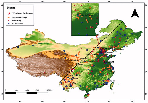
The observation wells (Figure 1) are mainly distributed in the lower right corner, to the right of the black dashed line, while the Qinghai–Tibet Plateau and its margins have only a few wells though there is strong seismic activity in the region. The inset diagram shows the capital region with the maximum density of wells. The yellow rhombuses indicate the step-like (including step-like rise and step-like fall) changes in water level, the red triangles indicate the oscillatory changes in water level, and the blue circles represent no changes in water level at the time when the Wenchuan earthquake occurred. The red pentagram shows the epicenter of the Wenchuan earthquake, which is located on the edge of the Qinghai–Tibet Plateau. The stations mentioned in this paper are shown and labelled with the station name.

Groundwater level monitoring is implemented using two types of instruments. The first instrument is an analogue water level recorder that provides a continuous curve; with this instrument, the observer reads 24-hour data daily. The second instrument is a digital piezometer, and data are logged in 1-min intervals. These instruments have an accuracy of 1 cm and a resolution of 1 mm. Obviously, these instruments cannot record hydroseismograms (He et al. 2017a) since the periods of hydroseismograms range from several seconds to tens of seconds. In this article, we do not pay attention to the hydroseismograms process; instead, we have only considered co-seismic and post-seismic events.

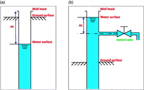
There are two types of groundwater level observation wells in mainland China. The first type is the non-artesian well, and the second type is the flowing artesian well (Figure 2). For the non-artesian well, the water level is defined as the distance from the water surface of the borehole to the well head (Figure 2a). In contrast, for the artesian well, the water flow is controlled by a control valve that maintains the water surface within a certain range (i.e. the water surface remains at the axis of the control valve if the flow discharge is too high, or the water will be output from the well head and the water surface remains at the well head if the flow discharge is too low). The water level is defined as the distance between the well water surface and the axis of the valve (Figure 2b).

Figure 2. Two types of observation wells in mainland China (a) Non-artesian well: the observed water level is defined as the distance between the well head and the water surface. In general, the Y-axis need be reversed when the water level of a non-artesian well is plotted. (b) Artesian well: the observed water level is determined as the distance between the axis of the valve and the water surface.

3. Methods

3.1. Eliminating of disturbance components

The water level dynamic can often be expressed as (Matsumoto 1992; Matsumoto et al. 2003; He et al. 2016): (1) $$y_n=x_n+P_n+T_n+{\epsilon }_n$$(1)

where$y_n$ is the observed water level value, $x_n$ is the final water level value (and includes rainfall and earthquake activities), $P_n$ is associated with the atmospheric pressure, $T_n$is the earth tidal effect, and ${\epsilon }_n$ is the measurement noise. ${\epsilon }_n$ is assumed as the Gauss white noise, of which the average is zero with a variance ${\sigma }^2$. In this paper, we used the partial least squares (PLS) method to remove the earth tidal and atmospheric pressure effects on water level (He et al. 2016).

The $T_n$ and $P_n$ data expressed in Equation (1)(1) $$y_n=x_n+P_n+T_n+{\epsilon }_n$$(1) can be expressed as Equation (2)(2) $$\{\begin{array}{c}{T}_n=k_t*t_n+b_t\\ P_n=k_p*p_n+b_p\end{array}$$(2) : (2) $$\{\begin{array}{c}{T}_n=k_t*t_n+b_t\\ P_n=k_p*p_n+b_p\end{array}$$(2)

where $k_t$ is the earth tidal response coefficient, $t_n$ is the theoretical value of the volumetric tidal strain, $k_p$ is the atmospheric pressure response coefficient, $p_n$ is the observed atmospheric pressure value, $b_t$ and $b_p$are constants.

First, it is necessary to select a data observational period ($\ge 30$days) that is free from anthropogenic disturbances and seismic actives to compute the effect factors. Second, the significant error data must be removed (e.g. the single jump point), the missing data must be complemented by cubic polynomial interpolation, and the linear trend must be removed (Figure 3a). Third, the earth tidal effect must be eliminated, and the tidal factor,$k_t$, must be calculated by PLS (Figure 3b). Fourth, the atmospheric pressure effect must be removed, and the air pressure factor, $k_p$, must be calculated by PLS (Figure 3c). In fact, we need to simultaneously remove the tidal and air pressure effects (i.e. combine the third and the fourth steps) because the atmospheric pressure often includes the tidal influence. After the above steps are complete, we can determine the ‘pure’ water level fluctuations (Figure 3d) and the effect factors (Kt, Kp) for the subsequent calculation.

Figure 3. Eliminating disturbance components.

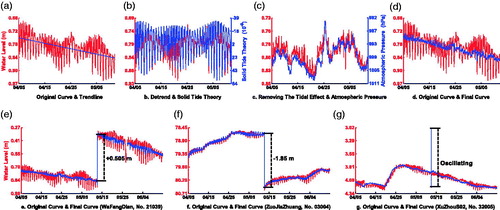
Using the above factors (Kt, Kp), the disturbance components of the water level can be eliminated, and the type of co-seismic response, i.e. step-like change (includes step-like rise (Figure 3e) and step-like fall (Figure 3f)), oscillation (Figure 3g), and no response, can be identified. To search for any potential spatially coherent signals, we quantitatively analyzed the step-like changes, in which a positive result indicated a step-like rise and a negative result indicated a step-like fall.

We have eliminated disturbances following steps:

1. Step 1: select the original observation data and plot the trend line. In this paper, we selected the WaFangDian station for illustrating this calculation.

2. Step 2: after removing the linear trend, we can clearly see the tidal effect on the water level (red line – water level; blue line – earth tide), and we can use PLS to remove the tidal component.

3. Step 3: after removing the tidal effect, we can clearly see the atmospheric pressure effect on the water level (red line – water level; blue line –atmospheric pressure), and we can use PLS to remove the air pressure component.

4. Step 4: we obtain the final water level and the effect factors (Kt, Kp). In fact, we need to simultaneously remove the tidal and air pressure effects (by combining the third and the fourth steps) because the atmospheric pressure often includes the tidal influence.

5. The step-like co-seismic change (i.e. a step-like rise) is shown at the WaFangDian station (station code: 21039). The term ‘+0.505 m’ indicates the water level step-rise was 0.505 m when the Wenchuan earthquake occurred.

6. The step-like co-seismic change (i.e. a step-like fall) is shown at the ZuoJiaZhuang station (station code: 03004). The term ‘−1.85 m’ indicates the water level step-fell by 1.85 m when the Wenchuan earthquake occurred.

7. The oscillation is shown at the XinZhouS02 station (station code: 32005). The amplitude of oscillation is distorted because the sampling rate ranges from less than several seconds to more than tens of seconds, which is based on the period of hydroseismograms.

3.2. Comparison of tidal parameters between pre- and post-seismic conditions

Short-period earth tides (Table 1) mainly include semi-diurnal waves (M₂, S₂, N₂, K₂) and diurnal waves (K₁, O₁, P₁) (Wallima 2007). In this paper, we consider only the M₂ wave to quantitatively calculate the change in amplitude and the phase shift (Bredehoeft 1967; Carr and Van Der Kamp 1969; Bower and Heaton 1978).

Table 1. The main earth tidal waves.

	Symbol	Period		Symbol	Period
Semi-diurnal	M2	12 h 25 m	Diurnal	K1	23 h 56 m
	S2	12 h 00 m		O1	25 h 49 m
	N2	12 h 39 m		P1	24 h 04 m
	K2	11 h 58 m

We adopted the t_tide toolbox, which was provided by Pawlowicz et al. (2002), to compute the amplitude and the phase of the M₂ wave, and we used Equation 3(3) $$\mathrm{r}=\frac{{\mathrm{A}}_{\text{po}}-{\mathrm{A}}_{\text{pr}}}{{\mathrm{A}}_{\text{pr}}}\times 100\%$$(3) to compute the change ratio of the amplitude: (3) $$\mathrm{r}=\frac{{\mathrm{A}}_{\text{po}}-{\mathrm{A}}_{\text{pr}}}{{\mathrm{A}}_{\text{pr}}}\times 100\%$$(3)

where $\mathrm{r}$ is the change ratio of the amplitude, and ${\mathrm{A}}_{\text{po}}$ and ${\mathrm{A}}_{\text{pr}}$ are the amplitudes before and after the Wenchuan earthquake, respectively. We selected the observation data from 12 April to 11 May, 2008 as pre-seismic data and from 12 May to 11 June, 2008 as post-seismic data for calculations.

3.3 Post-seismic groundwater recession

The post-seismic water level adjustment or recovery (Stein and Lisowski 1983) is called ‘post-seismic groundwater recession’ (Wang and Manga 2010). After a sufficient period of time, the water level has a time-dependent relation (Wang and Manga 2010): (4) $$\text{log}\hspace{0.17em}h=a-bt$$(4)

Here, $h$ is the post-seismic water level residual, $a$ and $b$ are obtained by linear fitting of the post-seismic water level with time, and the negative sign in front of $b$ indicates that $b$ is a positive number itself. The terms $b$ and $c$ (the base flow recession constant) are physically equivalent, and the characteristic time is: (5) $$\tau \equiv 1/b$$(5)

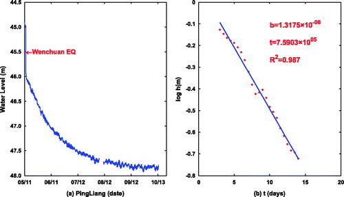
Using PingLiang station as an example, we can calculate the recession constant and the characteristic time by the least squares fit (Figure 4), and the coefficient of determination (R²) is 0.987.

Figure 4. Post-seismic groundwater recession (a) The blue line is the original water level at the PingLiang station from 11 May to 15 October, 2008. The direction of the y-axis is reversed to indicate a non-artesian well. (b) The logarithmic post-seismic residual of water level against time for PingLiang station. The red dots are daily averages, and the blue straight line is the least square linear fit to the data.

4. Results and analysis

4.1. The spatial characteristic of the co-seismic response

There were 280 wells to analyse, including 138 wells (49%) with step-like changes, 69 wells (25%) with oscillations and 73 wells (26%) with no response. The spatial quantifications of step-like changes are shown in Figure 5.

Figure 5. Diagrams showing the spatial quantifications of step-like changes.

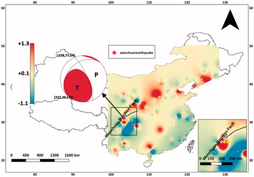
Red means step-like rises, and blue represents step-like decline in water level when the Wenchuan earthquake occurred; additionally, the shade of the colour represents the change in amplitude (see the colour band). The red pentagram is the epicenter, and the ball is the focal mechanism solution of the Wenchuan earthquake. The inset displays the epicenter region, and the black line is the Wenchuan–MaoWen fault. No spatially coherent signal was found—even around the epicenter—through the spatial interpolation analysis. We did not analyse the spatial characteristics in western China because this area has only a few observation wells.

Spatial interpolation analysis was carried out, except in region with few wells (e.g. western China) (Figure 5). The randomness of the step-like change is seen clearly, and no spatially coherent signal was found, even around the epicenter.

In addition, the relationship between amplitude and well-epicenter distance is shown in Figure 6. There were only two wells within 200 km of the epicenter, and all other wells belonged to the intermediate field. The step-like changes were strongly random when the epicenter distance was less than 1800 km, but almost all values were positive when the distance was greater than 1800 km; this characteristic was either independent or needs more data to confirm. The amplitudes of the step-like changes were mainly distributed between −0.5 m and 0.5 m, but this range did not depict a completely normal distribution.

Figure 6. The relationship between amplitude and well-epicenter distance (a) In terms of the y-axis (amplitude), a positive value is a step-like rise, and a negative value is a step-like fall. The blue dotted line marks 1800 km of epicentral distance. The distribution of positive or negative is random when the well-epicenter distance was less than 1800 km, but almost all values were positive when the distance was greater than 1800 km. (b) The probability distribution is shown. The amplitude of step-like changes was mainly within [−0.5 m to 0.5 m].

4.2. The changes in tidal parameters between pre- and post-seismic conditions

The phase shifts in the water level response to the tidal strain (M₂ wave) of post-seismic conditions always occur before seismic conditions (Elkhoury et al. 2006), but the changes in amplitude (M₂ wave) were random (Figure 7). In addition, the phase shifts were concentrated at $0.23\pi \sim 0.4\pi$ (i.e. the pink frame in Figure 7), regardless of the epicenter distance. The tidal effect disappeared in a few wells (e.g. the QiXian well) due to the Wenchuan earthquake.

Figure 7. The changes in tidal parameters between pre- and post-seismic conditions.

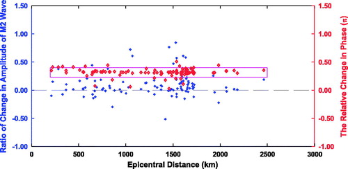
Blue dotes represent the ratio of change in water level of the amplitude of M₂ wave, as calculated by Equation 3(3) $$\mathrm{r}=\frac{{\mathrm{A}}_{\text{po}}-{\mathrm{A}}_{\text{pr}}}{{\mathrm{A}}_{\text{pr}}}\times 100\%$$(3) . Positive values indicate an increase, and negative values indicate a decrease in the amplitude. The red dots show the phase shift, and positive values mean advances, and negative values mean lags. The random changes in amplitude are seen clearly, and the phase shift is concentrated at $0.23\pi \sim 0.4\pi$ (i.e. the pink frame).

4.3. The results of post-seismic groundwater recession

Some recession constants ($b$) and characteristic times ($\tau$), which were calculated by Equation 4(4) $$\text{log}\hspace{0.17em}h=a-bt$$(4) , are shown in Table 2.

Table 2. A selection of recession constants and characteristic times.

Station code	Station name	$b$	$\tau$	$R^2$	Station code	Station name	$b$	$\tau$	$R^2$
13105	HuangHua	4.36E-06	2.29E + 05	0.976	51069	NanXi	9.93E-07	1.01E + 06	0.97
14028	QiXian	−4.34E-07	−2.30E + 06	0.98	53053	PuEr	8.13E-07	1.23E + 06	0.998
14036	JieXiu	1.34E-06	7.48E + 05	0.99	53142	MiLe	−9.71E-07	−1.03E + 06	0.98
35045	PingTan	−3.96E-07	−2.52E + 06	0.99	61009	XiGuang	−5.52E-07	−1.81E + 06	0.995
44022	MeiZhou	−2.83E-07	−3.54E + 06	0.97	61059	LuoNan	6.92E-07	1.44E + 06	0.993
50504	DaZu	−8.87E-07	−1.13E + 06	0.99	62009	PingLiang	5.65E-07	1.77E + 06	0.987
51065	XiChang	1.22E-06	8.21E + 05	0.99	62132	QingShui	−3.08E-07	−3.25E + 06	0.997
51068	PanZhiHua	−3.89E-07	−2.57E + 06	0.99

5. Theoretical analysis and discussion

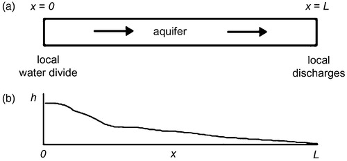
In mainland China, most observation wells are equipped with casing that is $70\sim 100\mathrm{m}$ from the ground surface, and wells have an impermeable grout seal around the casing that can prevent the interference of surface water. In general, the water level in a well is mainly determined by the main-confined aquifer, although the observation well may penetrate many aquifers due to permeability or thickness. Therefore, we can simplify the well-aquifer system to a one-aquifer model and ignore the non-dominant aquifers. Here, we adopted a first-order approximation, i.e. a one-dimensional aquifer model (Figure 8), which was provided by Wang and Manga (2010).

Figure 8. The simplified one-aquifer model (Wang and Manga 2010) (a) The geometry of the model aquifer and its boundaries: a local water divide (recharge area) is located at $x=0$, and a local discharge is located at $x=L$. (b) Schematic drawing to show the boundary conditions used to solve Equation 6: head ‘$h$’ is zero at the local discharge ($x=L$), and the gradient of the head is zero at the local water divide ($x=0$).

We assumed the length of the aquifer was $L$, the characteristic time was $\tau$ (computed from the recession analysis), and the water head was $h$ (Figure 8). The boundaries were a local water divide (recharge) located at $x=0$, and a local discharge was located at $x=L$. The boundary conditions were $h=0$ at the local discharge ($x=L$), and the gradient of the water head was zero at the local water divide ($x=0$). The water head at $x$ against time $t$ can be calculated as: (6) $$h\left(x,t\right)=\frac{4A_0}{\pi S_s}\sum _{r=1}^{\infty }\frac{{\left(-1\right)}^{r+1}}{\left(2r-1\right)}\text{cos}\hspace{0.17em}\frac{\left(2r-1\right)\pi x}{2L}\text{exp}\hspace{0.17em}\left[-{\left(2r-1\right)}^2\frac{t}{\tau }\right]$$(6)

where $A_0$ is the amount of earthquake-induced recharge to the aquifer per unit volume, $S_s$ is the specific storage, and $x/L$ indicates the observation well situation at the aquifer.

Using this single-aquifer model, Wang et al. (2004) compared the predictions (color curves in Figure 9) using Equation 6(6) $$h\left(x,t\right)=\frac{4A_0}{\pi S_s}\sum _{r=1}^{\infty }\frac{{\left(-1\right)}^{r+1}}{\left(2r-1\right)}\text{cos}\hspace{0.17em}\frac{\left(2r-1\right)\pi x}{2L}\text{exp}\hspace{0.17em}\left[-{\left(2r-1\right)}^2\frac{t}{\tau }\right]$$(6) and the observation data (i.e. the black dots in Figure 9) at the Yuanlin I well, and $\mathrm{x}/\mathrm{L}=0.5$ was considered an excellent fit; this represents the observation well in the middle of the aquifer.

Figure 9. Comparing the prediction by Equation 6 and the observation data at the Yuanlin I well (Wang et al. 2004).

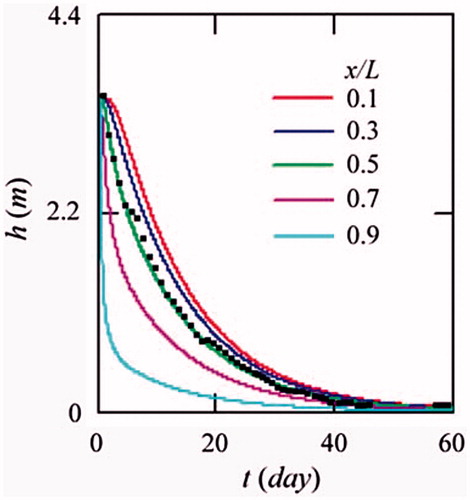
Black dots show data points. Model prediction of post-seismic changes in h are shown by the coloured curves for several values of x/L. An excellent fit between the data and the curve occurs at x/L = 0.5.

Meanwhile, we conclude that the smaller $x/L$ values have a smaller radian of the prediction curve, and the larger $x/L$ values have a larger radian of the prediction curve. In fact, the radian implicates the recharge or discharge ability of the observation well through the aquifer, i.e. a smaller radian means stronger recharge ability from the water divide (recharge area) to the observation well through the aquifer, and a larger radian indicates stronger discharge ability from the observation well to the discharge area (river, stream, reservoir, etc.) through the aquifer. These different abilities (i.e. recharge or discharge) will play a dominant role in the co-seismic response of water levels in the observation wells.

According to the Darcy’s Law: (7) $$Q=KA\frac{H1-H2}{L}=KAI$$(7)

where $Q$ is the total discharge (${\mathrm{m}}^3/\mathrm{d}$), $\mathrm{K}$ is the hydraulic conductivity ($\mathrm{m}/\mathrm{d}$), $\mathrm{A}$ is the cross-sectional area to flow (${\mathrm{m}}^2$), $H1-H2$ is the hydraulic head drop (m), $\mathrm{L}$ is the length over which the head drop is taking place (m), and $I$ is the hydraulic gradient.

The seismic waves enhanced the permeability ($k,K=\frac{\rho g}{u}k$) by removing precipitates and colloidal particles from clogged fractures, which caused the total discharge, $Q,$ to increase. Meanwhile, the water must overcome the friction between the water and the ‘tube wall’ as well as the water particles of different velocities when it flows in the gaps of the aquifer. The friction will increase with the increase in groundwater flow velocity and consume the mechanical energy of the water flow. The effect of the increase in permeability will be neutralized with the friction if the flow-path is of sufficient length.

The radian of the prediction curve of the post-seismic adjustment (Figure 9) will be smaller when the observation well is closer to the recharge area and farther from the discharge area. In other words, the recharge ability between the observation well and the recharge area will significantly improve as the permeability is enhanced, which is induced by the seismic wave. However, the discharge ability between the observation well and the discharge area will be almost maintained at the pre-seismic level because the friction neutralizes the increase in permeability. As a result, the excess water will be stored around the observation well and will induce a step-like rise when the seismic waves arrive.

The seismic waves enhance the permeability, which means that the water from the local water source (recharge area) will be transmitted to the observation well easier if the observation well is closer to the recharge area and farther away from the discharge area (Figure 10). Meanwhile, the transmission capability between the well and the discharge area almost remain at the original (pre-seismic) level because the friction neutralizes the increase in permeability due to the long seepage flow-path. Obviously, the excess recharge will be stored around the observation wells for a period of time (hours, days, or even months) (Roeloffs et al. 2003; Ogawa and Heki 2007; Cox et al. 2012). In this case, the co-seismic response of water level will show the ‘step-like rise’ and may maintain the rise or the recovery of the post-seismic adjustment (Sil and Freymueller 2006); this is determined by the distance between the well and the discharge area. There is a special case, i.e. the QiongLai well, which is located in Sichuan Province with a distance to the epicenter of the Wenchuan earthquake of approximately 267 km; this well was a flowing artesian well before 2007 and become a non-flow well. However, the QiongLai well resumed flow after the Wenchuan earthquake.

Figure 10. The step-like co-seismic changes determined by the proximity of wells to recharge or discharge areas.

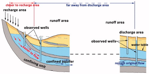
In contrast, the observation well will undergo excessive discharge but will maintain its original recharge through increases in permeability if the observation well is closer to the discharge area and farther away from the recharge area. In this case, the co-seismic response of water level will show the ‘step-like’ fall and may maintain the falling or the recovery of the post-seismic adjustment.

The discharge or recharge capability of an observation well will not be affected when the observation well is farther away from the recharge area and the discharge area, even if the seismic waves enhance permeability. In this case, the water level will oscillate as the groundwater flows in and out of the aquifer when the seismic waves arrive (Cooper et al. 1965; Liu et al. 1989; Kitagawa et al. 2006). Of course, the water level will remain constant if the observation well does not penetrate any confined aquifer, even in the presence of strong ground shaking.

These conclusions are consistent with the calculation results of a one-dimensional aquifer model (Equation 6(6) $$h\left(x,t\right)=\frac{4A_0}{\pi S_s}\sum _{r=1}^{\infty }\frac{{\left(-1\right)}^{r+1}}{\left(2r-1\right)}\text{cos}\hspace{0.17em}\frac{\left(2r-1\right)\pi x}{2L}\text{exp}\hspace{0.17em}\left[-{\left(2r-1\right)}^2\frac{t}{\tau }\right]$$(6) ), the post-seismic phase shifts of the M₂ wave, and the similar morphological change in water level associated with multiple earthquakes in the one observation well (Yang 2004; Weingarten and Ge 2014; Lai et al. 2016).

Acknowledgments

The authors thank the China Earthquake Network Center for providing the groundwater level data and station information. The original data can be found in zenodo (DOI:zenodo.1038140).

Disclosure statement

No potential conflict of interest was reported by the authors.

Additional information

Funding

The present study was financially supported by the National Natural Science Foundation of China (No. 41772256) and the Research grants from Institute of Crustal Dynamics, China Earthquake Administration (No. ZDJ2017-25).

References

- Akita F, Matsumoto N. 2004. Hydrological responses induced by the Tokachi–Oki earthquake in 2003 at hot spring wells in Hokkaido, Japan. Geophys Res Lett. 31(16):371–375.
- Blanchard FB, Byerly P. 1935. A study of a well gauge as a seismograph. Bull Seismol Soc Am. 25(4):313–321.
- Bower DR, Heaton KC. 1978. Response of an aquifer near Ottawa to tidal forcing and the Alaskan earthquake of 1964. Can J Earth Sci. 15(3):331–340.
- Bredehoeft JD. 1967. Response of well—aquifer systems to Earth tides. J Geophys Res. 72(12):3075–3087.
- Brodsky EE, Roeloffs E, Woodcock D, Gall I, Manga M. 2003. A mechanism for sustained groundwater pressure changes induced by distant earthquakes. J Geophys Res. 108(B8):503–518.
- Carr PA, Van Der Kamp GS. 1969. Determining aquifer characteristics by the tidal method. Water Resour Res. 5(5):1023–1031.
- Chan CH, Wang Y, Almeida R, Yadav RBS. 2017. Enhanced stress and changes to regional seismicity due to the 2015 M w 7.8 Gorkha, Nepal, earthquake on the neighbouring segments of the Main Himalayan thrust. J Asian Earth Sci. 133:46–55.
- Chia Y, Wang YS, Chiu JJ, Liu CW. 2001. Changes of groundwater level due to the 1999 Chi-Chi earthquake in the Choshui River alluvial fan in Taiwan. Bull Seismol Soc Am. 91(5):1062–1068.
- Cooper HH, Bredehoeft JD, Papadopulos IS, Bennett RR. 1965. The response of well-AQUIFER systems to seismic waves. J Geophys Res. 70(16):3915–3926.
- Cox SC, Rutter HK, Sims A, Manga M, Weir JJ, Ezzy T, White PA, Horton TW, Scott D. 2012. Hydrological effects of the Mw 7.1 Darfield (Canterbury) earthquake, 4 September 2010, New Zealand. New Zealand J Geolog Geophys. 55(3):231–247.
- Cui XF, Hu XP, Yu CQ, Tao K, Wang Y, Ning J. 2011. Research on focal mechanism solutions of Wenchuan earthquake sequence. Acta Sci. Nat. Univ. Pekinensis. 6:1063–1072.
- Dobry R, Ladd RS, Yokel FY, Chung RM, Powell D. 1982. Prediction of pore water pressure buildup and liquefaction of sands during earthquakes by the cyclic strain method (Vol.138). Gaithersburg (MD): National Bureau of Standards.
- Elkhoury JE, Brodsky EE, Agnew DC. 2006. Seismic waves increase permeability. Nature. 441(7097):1135.
- Ge S, Stover SC. 2000. Hydrodynamic response to strike- and dip-slip faulting in a half-space. J Geophys Res. 105(B11):25513–25524.
- Geballe ZM, Wang CY, Manga M. 2011. A permeability-change model for water-level changes triggered by teleseismic waves. Geofluids. 11(3):302–308.
- Grecksch G, Roth F, Kümpel HJ. 1999. Coseismic well-level changes due to the 1992 roermond earthquake compared to static deformation of half-space solutions. Geophys J Int. 138(2):470–478.
- Gulley AK, Ward NFD, Cox SC, Kaipio JP. 2013. Groundwater responses to the recent Canterbury earthquakes: a comparison. J Hydrol. 504:171–181.
- He A, Fan X, Zhao G, Liu Y, Singh RP, Hu Y. 2017a. Co-seismic response of water level in the Jingle well (China) associated with the Gorkha Nepal (Mw 7.8) earthquake. Tectonophysics. 714–715:82–89.
- He A, Singh RP, Sun Z, Ye Q, Zhao G. 2016. Comparison of regression methods to compute atmospheric pressure and earth tidal coefficients in water level associated with Wenchuan Earthquake of 12 May 2008. Pure Appl Geophys. 173(7):2277–2294.
- He A, Zhao G, Sun Z, Singh RP. 2017b. Co-seismic multilayer water temperature and water level changes associated with Wenchuan and Tohoku-Oki earthquakes in the Chuan no. 03 well, China. J Seismol. 21(4):719–734.
- Hsu CC, Vucetic M. 2004. Volumetric threshold shear strain for cyclic settlement. J Geotech Geoenviron Eng. 130(1):58–70.
- Itaba S, Koizumi N, Matsumoto N, Takahashi M, Sato T, Ohtani R. 2008. Groundwater level changes related to the ground shaking of the Noto Hanto earthquake in 2007. Earth Planet Space. 60(12):1153–1159.
- Jonsson S, Segall P, Pedersen R, Bjornsson G. 2003. Post-earthquake ground movements correlated to pore-pressure transients. Nature. 424(6945):179.
- King CY, Azuma S, Igarashi G, Ohno M, Saito H, Wakita H. 1999. Earthquake-related water-level changes at 16 closely clustered wells in Tono, Central Japan. J Geophys Res. 104(B6):13073–13082.
- Kitagawa Y, Koizumi N, Takahashi M, Matsumoto N, Sato T. 2006. Changes in groundwater levels or pressures associated with the 2004 earthquake off the west coast of northern Sumatra (M9. 0). Earth Planet Sp. 58(2):173–179.
- Koizumi N, Lai W, Kitagawa Y, Matsumoto N. 2004. Comment on “Coseismic hydrological changes associated with dislocation of the September 21, 1999 Chichi earthquake, Taiwan” by Min Lee et al. Geophys Res Lett. 31(13):n/a.
- Lai W-C, Koizumi N, Matsumoto N, Kitagawa Y, Lin C-W, Shieh C-L, Lee Y-P. 2004. Effects of seismic ground motion and geological setting on the coseismic groundwater level changes caused by the 1999 Chi-Chi earthquake, Taiwan. Earth Planet Sp. 56(9):873–880.
- Lai G, Jiang C, Han L, Sheng S, Ma Y. 2016. Co-seismic water level changes in response to multiple large earthquakes at the LGH well in Sichuan, China. Tectonophysics. 679:211–217.
- Lee M, Liu TK, Ma KF, Chang YM. 2002. Coseismic hydrological changes associated with dislocation of the September 21, 1999 Chichi earthquake, Taiwan. Geophys Res Lett. 29(17):5-1–5-4.
- Lee M, Liu TK, Ma KF, Chang YM. 2004. Reply to comment by N. Koizumi et al. on “Coseismic hydrological changes associated with dislocation of the September 21, 1999 Chichi earthquake, Taiwan. Geophys Res Lett. 31(13):n/a.
- Liu L, Tan G, Luan F, Tang X, Kang P, Tu C, Pei F. 2012. The use of external fixation combined with vacuum sealing drainage to treat open comminuted fractures of Tibia in the Wenchuan earthquake. Int Orthopaedic. 36(7):1441–1447.
- Liu LB, Roeloffs E, Zheng XY. 1989. Seismically induced water level fluctuations in the Wali Well, Beijing, China. J Geophys Res. 94(B7):9453–9462.
- Ma Y, Huang F. 2017. Coseismic water level changes induced by two distant earthquakes in multiple wells of the Chinese mainland. Tectonophysics. 694:57–68.
- Matsumoto N. 1992. Regression analysis for anomalous changes of ground water level due to earthquakes. Geophys Res Lett. 19(12):1193–1196.
- Matsumoto N, Kitagawa G, Roeloffs EA. 2003. Hydrological response to earthquakes in the Haibara well, central Japan–I. Groundwater level changes revealed using state space decomposition of atmospheric pressure, rainfall and tidal responses. Geophys J Int. 155(3):885–898.
- Merifield PM, Lamar DL. 1984. Possible strain events reflected in water levels in wells along San Jacinto fault zone, Southern California. Pure and Applied Geophysics. 122(2–4):245–254.
- Molnar P, Lyon-Caent H. 1989. Fault plane solutions of earthquakes and active tectonics of the tibetan plateau and its margins. Geophys J Int. 99(1):123–153.
- Montgomery DR, Manga M. 2003. Streamflow and water well responses to earthquakes. Science. 300(5628):2047–2049.
- Nur A, Booker JR. 1972. Aftershocks caused by pore fluid flow? Science. 175(4024):885–887.
- Ogawa R, Heki K. 2007. Slow postseismic recovery of geoid depression formed by the 2004 Sumatra – Andaman earthquake by mantle water diffusion. Geophys Res Lett. 34(6):n/a.
- Pawlowicz R, Beardsley B, Lentz S. 2002. Classical tidal harmonic analysis including error estimates in MATLAB using T_TIDE. Comput Geosci. 28(8):929–937.
- Peltzer G, Rosen P, Rogez F, Hudnut K. 1996. Postseismic rebound in fault step-overs caused by pore fluid flow. Science. 273(5279):1202–1203.
- Piombo A, Martinelli G, Dragoni M. 2005. Post-seismic fluid flow and Coulomb stress changes in a poroelastic medium. Geophys J Int. 162(2):507–515.
- Quilty EG, Roeloffs EA. 1997. Water-level changes in response to the 20 December 1994 earthquake near Parkfield, California. Bull Seismol Soc Am. 87(2):310–317.
- Radhakrishnan N, Patel P, Kulkarni MN. 2010. Post-seismic effect of Sumatra-Andaman earthquake on the western part of Indian plate. IUP J Earth Sci. 4(3):45–55.
- Ramana DV, Chadha RK, Singh C, Shekar M. 2007. Water level fluctuations due to earthquakes in Koyna-Warna region, India. Nat Hazards. 40(3):585–592.
- Roeloffs E. 1996. Poroelastic techniques in the study of earthquake-related hydrologic phenomena. In: Dmowska R, editor. Advances in geophysics. San Diego (CA): Academic Press; pp. 135–195.
- Roeloffs EA. 1998. Persistent water level changes in a well near Parkfield, California, due to local and distant earthquakes. J Geophys Res. 103(B1):869–889.
- Roeloffs E, Sneed M, Galloway DL, Sorey ML, Farrar CD, Howle JF, Hughes J. 2003. Water-level changes induced by local and distant earthquakes at long valley Caldera, California. J Volcanol Geothermal Res. 127(3–4):269–303.
- Rojstaczer S, Wolf S. 1992. Permeability changes associated with large earthquakes: An example from Loma Prieta, California. Geol. 20(3):211–214.
- Shi ZM, Wang GC, Liu CL, Mei JC, Wang JW, Fang HN. 2013. Coseismic response of groundwater level in the three gorges well network and its relationship to aquifer parameters. Chin Sci Bull. 58(25):3080–3087.
- Shi Z, Wang G. 2016. Aquifers switched from confined to semiconfined by earthquakes. Geophys Res Lett. 43(21):11,166–11,172. doi: 10.1002/2016GL070937.
- Sil S, Freymueller JT. 2006. Well water level changes in Fairbanks, Alaska, due to the great sumatra-andaman earthquake. Earth Planet Sp. 58(2):181–184.
- Stein RS, Lisowski M. 1983. The 1979 Homestead Valley earthquake sequence, California: Control of aftershocks and postseismic deformation. J Geophys Res. 88(B8):6477–6490.
- Sun X, Wang G, Yang X. 2015. Coseismic response of water level in Changping well, China, to the Mw 9.0 Tohoku earthquake. J Hydrol. 531:1028–1039.
- Vucetic M. 1994. Cyclic threshold shear strains in soils. J Geotech Eng. 120(12):2208–2228.
- Wakita H. 1975. Water wells as possible indicators of tectonic strain. Science. 189(4202):553–555.
- Wallima L. 2007. Fundamentals of geophysics. New York: Cambridge University Press.
- Wang CY, Cheng LH, Chin CV, Yu SB. 2001. Coseismic hydrologic response of an alluvial fan to the 1999 Chi-Chi earthquake, Taiwan. Geol. 29(9):831–834.
- Wang CY, Chia Y. 2008. Mechanism of water level changes during earthquakes: Near field versus intermediate field. Geophys Res Lett. 35(12):109.
- Wang CY, Manga M. 2010. Earthquakes and water. Lecture Notes in Earth Sciences 114, Berlin: Springer-Verlag.
- Wang CY, Wang CH, Kuo CH. 2004. Temporal change in groundwater level following the 1999 (Mw =7.5) Chi-Chi earthquake, Taiwan. Geofluids. 4(3):210–220.
- Weingarten M, Ge S. 2014. Insights into water level response to seismic waves: A 24 year high-fidelity record of global seismicity at Devils Hole. Geophys Res Lett. 41(1):74–80.
- Xu X, Wen X, Yu G, Chen G, Klinger Y, Hubbard J, Shaw J. 2009. Coseismic reverse-and oblique-slip surface faulting generated by the 2008 Mw 7.9 Wenchuan earthquake, China. Geology. 37(6):515–518.
- Xue L, Brodsky EE, Erskine J, Fulton PM, Carter R. 2016. A permeability and compliance contrast measured hydrogeologically on the San Andreas fault. Geochem Geophys Geosyst. 17(3):858–871.
- Yang ZZ. 2004. Water-level changes induced by earthquakes and a preliminary study of their mechanism [Doctoral dissertation]. Beijing: Institute of Geology, CEA.
- Yoshimi Y, Oh-Oka H. 1975. Influence of degree of shear stress reversal on the liquefaction potential of saturated sand. Soil Foundation. 15(3):27–40.
- Zhang Y, Fu LY, Huang F, Chen X. 2015. Coseismic water-level changes in a well induced by teleseismic waves from three large earthquakes. Tectonophysics. 651–652:232–241.
- Zheng J, Jiang H, He Z. 2012. Analysis of the co-seismic responses of the fluid well pattern system in Jiangsu Province to the Wenchuan and Tohoku earthquakes. Earthq Sci. 25(3):263–274.