Modelling temporal variation of fire-occurrence towards the dynamic prediction of human wildfire ignition danger in northeast Spain

Abstract

Models of human-caused ignition probability are typically developed from static or structural points of view. This research analyzes the intra-annual dimension of fire occurrence and fire-triggering factors in NE Spain and moves forward towards more accurate predictions. Applying the Maximum Entropy algorithm (MaxEnt) and using wildfire data (2008–2011) and GIS and remote sensing data for the explanatory variables, we construct eight occurrence data scenarios by splitting wildfire records into the four seasons and then separating each season into working and non-working days. We assess model accuracy using a cross-validation k-fold procedure and an operational validation with 2012 data. Results report a substantial contribution of accessibility across models, often coupled with Land Surface Temperature. In addition, we observe great temporal variability, with WAI strongly influencing winter models, whereas distance to roads stands out during working days. Model performances stand consistently above 0.8 AUC in all temporal scenarios, with outstanding predictive effectiveness during summer months. The comparison among static-to-dynamic approaches reveals superior performance of simulations considering temporal scenarios, with AUC values from 0.7 to 0.85. Overall, we believe our approach is reliable enough to derive dynamic predictions of human-caused fire occurrence.

Highlights

• Wildfires exhibit differential spatial patterns at seasonal and daily levels.

• Accessibility by road and human pressure on wildlands govern ignition probability.

• Dynamic modelling through temporal scenarios enhances prediction.

• Winter fires display a stronger relationship to agricultural activities (WAI).

Keywords:

• Wildfire
• ignition danger
• human drivers
• temporal dimension
• MaxEnt
• Spain

1. Introduction

According to MAPAMA (2012), preventive measures of wildfire suppression deserve increased attention both in national and international forums after having achieved high development and adequate efficacy over the last decade. In the same line, FAO’s Fire Management Voluntary Guidelines state that ‘Fire prevention may be the most cost-effective and efficient mitigation programme an agency or community can implement’ (FAO 2006, p. 28). In a broad sense, preventing a fire means stopping it before it ever happens. When it comes to wildfire prevention, several strategies such as awareness campaigns, preventive silviculture, or risk mitigation are usually employed (MAPAMA 2012). A key resource for risk mitigation is risk zoning and mapping (Koutsias et al. 2016), a subject in which Geographic Information Systems (GIS) (Chuvieco et al. 2003; Martínez et al. 2004; Vilar del Hoyo et al. 2008; Chuvieco et al. 2010, 2014), remote sensing (Allgöwer et al. 2003; Sesnie et al. 2008; Chowdhury and Hassan 2013) and spatial statistics and models (Bar Massada et al. 2013; Martínez-Fernández et al. 2013; Rodrigues et al. 2014; Rodrigues and de la Riva 2014a) have been traditionally involved.

The term ‘wildfire risk’ refers to the chance of fire starting and spreading (danger), as well as its potential damage over environmental and human resources (vulnerability). The concept of ‘wildfire danger’ describes the ‘factors affecting the inception, spread and resistance to control’. Therefore ‘wildfire danger’ is a component of ‘wildfire risk’ (NWCG 2018). Following this approach, we assess wildfire danger ignition, which is often influenced by various factors: weather conditions, causative agents and even potential damage, but most commonly the latter is not considered in operational wildfire danger assessments (San Miguel-Ayanz et al. 2003).

Wildfire ignition modelling has evolved over time and nowadays a number of models combine geographic information with remote sensing data in order to produce dynamic fire ignition predictions (Chowdhury and Hassan 2013, 2015). Many of these operational wildfire ignition forecasting systems across the world are primarily based on meteorological variables (Allgöwer et al. 2003; Abbott et al. 2007; Jolly et al. 2015) or related inputs like Fire Weather Index (FWI; Chelli et al. 2015). Human influence on fire ignition is usually disregarded, even though it is widely recognized that human beings act as fire initiators of most fire events in Mediterranean environments (Martínez et al.,2009). Human-related drivers of wildfires contain a temporal dimension which often requires a historical/temporal perspective (Zumbrunnen et al. 2011; Carmona et al. 2012). Nonetheless, the temporal perspective of human-related drivers is frequently neglected and these drivers enter the modelling as structural ‘static’ components, which means they have no temporal variation in its influence as fire-triggering factors. Recent studies by Rodrigues et al. (2016) and Vilar et al. (2016) report changes in human-related drivers over time and across space. According to this, the common approach for modelling human-caused wildfire ignition probability based on ‘static’ human factors may not be the most adequate solution. For instance, wildfire occurrence in Spain experiences two main peaks of activity within the year, one around the beginning of the spring (March) and the other during the summer (July) (MAPAMA 2012). Daily variations have been also observed, with preference towards wildfire occurrence during weekends (San-Miguel Ayanz and Camia 2009). Altogether, we believe there is sufficient evidence for moving towards the dynamic prediction of fire ignition, not only regarding its environmental component but considering the spatiotemporal variability of human activity.

Chuvieco et al. (2014) developed an operational framework for integrated wildfire risk assessment (danger plus vulnerability) based on GIS and remote sensing. The study presented dynamic (daily) risk maps for mainland Spain. However, the conceptual approach of Chuvieco et al. (2014) still relied on static human drivers based on long-term historical wildfire records. In recent years, several methods for human-caused wildfire risk assessment have been developed using historical records, although based on different methodological schemes, variables and scales. Without being exhaustive, some of the more recent efforts in Spain have explored logistic regression (Vilar del Hoyo et al. 2008; Martínez et al. 2009; Padilla and Vega-García 2011; Costafreda-Aumedes et al. 2018), Classification and Regression Trees (Amatulli et al. 2006; Verdú et al. 2012), Geographically Weighted Regression (Martínez-Fernández et al., 2013; Rodrigues et al. 2014) and Machine Learning approaches such as Random Forest, Boosted Regression Trees, Support Vector Machines (Rodrigues and de la Riva 2014b) or Maximum Entropy Models (MaxEnt; Vilar et al., 2016). A recent work by Costafreda-Aumedes et al. (2017) provides an up-to-date review of the main methods and variables available. As fire regimes are strongly dependent on human activities (Archibald et al. 2013; Salis et al. 2014), introducing this extensive knowledge of human drivers of wildfire danger into dynamic predictions is an opportunity still largely unexplored.

This work is therefore based on the notion of the differential temporal patterns of human-caused wildfires. We understand that time (month, day of the week, etc.) plays a substantial role in the overall ignition probability, as well as in the factors that condition this probability. This is driven by spatio-temporal dimensions of human activities, as these are determined by daily cycles (commuting), weekly cycles (working day vs. non-working day) and monthly and seasonal cycles (winter vs. summer, wildfire season, etc.). The aim of this study is the creation of seasonal (winter, spring, summer and fall) and day-type (working day vs. non-working day) models that account for the differential spatio-temporal behaviour of human-related driving factors over wildfire ignition probability in the northeast of Spain. Our work therefore intends to move one-step forward towards achieving more accurate predictions and ultimately developing more efficient dynamic predictive models. To do so, we propose a new methodological approach combining the dynamism of some fire drivers (fuel conditions) with the specific temporal variability of human activity. The novelty of our proposal lies in the design and application of dynamic models based on specific scenarios of fire occurrence, presence-only methods (MaxEnt) and high resolution spatial datasets to account for fire ignitions and human-related wildfire drivers. The performance of these dynamic models was evaluated against random background samples (wildfire absence) and throughout a comparison of their predictive capacity with static models using wildfire data from 2012. Overall, dynamic models outperform the static (and semi-static) approach, reporting AUC values consistently above 0.85 compared to 0.7 observed in static models.

2. Materials and methods

The methodology for the creation of dynamic models of human wildfire ignition probability was developed in three stages. First, (i) we constructed eight intra-annual occurrence scenarios based on the observed distribution at seasonal – winter, spring, summer and fall – and daily levels – working vs. non-working days. Then, (ii) we calibrated and validated a predictive model for each scenario. Finally, (iii) we performed dynamic predictions at a daily level which are, in turn, validated from an operational standpoint using real wildfire occurrence data.

Model calibration and validation was based on the Maximum Entropy model (MaxEnt). Specifically, we used MaxEnt software, version 3.4.1k (Phillips et al. 2006, https://www.cs.princeton.edu/∼schapire/maxent/). We developed the operational prediction and validation using the equivalent MaxEnt R package.

2.1. Study area

The study area covers an extensive area of the northeast of Spain. The selection of the Spanish provinces of Huesca, Zaragoza, Lleida, Barcelona and Tarragona (Figure 1) includes different environments -both human and natural- that can be found in the Mediterranean region. These 59,081 km², representing 11.7% of the Spanish national territory, comprise traditional rural areas, especially notable in the provinces of Zaragoza and Huesca, and highly populated and urbanized regions such as the Mediterranean coast and the metropolitan area of Zaragoza. It also contains mountain areas with peaks over 3000 meters above sea level and a fair portion of Mediterranean coastline, which accounts for ecological and climatic variations ranging from mountain ecosystems to sub-arid Mediterranean environments. Table 1 shows the variability of the study area. This spatial heterogeneity of natural and socioeconomic conditions, which determines the differential patterns of human ignition factors, is therefore well reflected and considered in this article, leaving for further research the possibility of extending the study region.

Figure 1. Study area. Source: National (Spain) Geographic Institute.

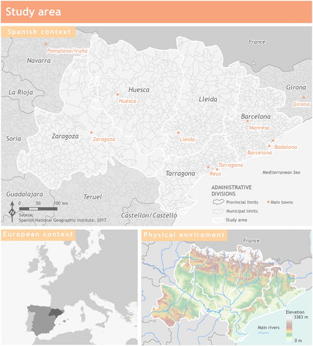
Table 1. Characteristics of the provinces comprising the study area.

	Area (km²)	Population (2017)	Population density (inh/km²)	GDP	Mean altitude (m)
Barcelona	7782	5,576,037	716.53	27,813	516
Huesca	15,626	219,702	14.06	25,386	851
Lleida	12,028	432,384	35.95	28,360	934
Tarragona	6303	791,693	125.61	28,122	339
Zaragoza	17,274	953,486	55.20	25,423	714

2.2. Overview of the MaxEnt algorithm and software

MaxEnt is a general-purpose algorithm that assists in the creation of models with incomplete information. Applied to wildfire modelling, MaxEnt is able to run with presence data, without needing a random point cloud as absence background (Bar Massada et al. 2013). MaxEnt models are based on the iterative comparison of the predictive (independent) variable values in the locations of occurrence (presence) with a vast subsample extracted from the study area, and that is used as non-occurrence values (Phillips et al. 2006; Elith et al. 2011). MaxEnt has already been used in modelling ignition probability studies in the United States (Parisien and Moritz 2009), in India (Renard et al. 2012), and China (Chen et al. 2015), among other regions.

MaxEnt estimates the target distribution probability of an event by adjusting the probability distribution of the maximum entropy. In other words, it adjusts the probability to the most uniform or spread out distribution according to the independent variables in each point of observation (Phillips et al. 2006). Therefore, similar to other probability modelling algorithms, MaxEnt requires two sets of data. First, a dependent variable is needed, which in our case is wildfire presence/occurrence data. Second, a set of predictor variables (independent variables) is required.

One of the essential characteristics of MaxEnt is the capacity of adjusting highly complex response functions combining several types of functions (linear, quadratic, product, threshold and hinge). This allows modelling discontinuous responses that the most flexible regression models cannot adjust. In this sense, within the different modelling options available that are able to run with only presence data, MaxEnt has shown more accuracy in the forecast, especially with small sample sizes (Pearson et al. 2007; Elith et al. 2011).

MaxEnt software allows the user to generate probability (i.e. logistic) models producing several numerical and graphical outputs. MaxEnt can be set according to several parameters such as the number of iterations or the learning rate of the algorithm. It also performs a validation and sensitivity analysis based on AUC (Area Under the Curve) measures and a jack-knife procedure. The importance of the independent variables in each model is quantified and the software returns a raw probability model, including both the average predicted probability and the standard deviation of the prediction over the pre-set number of iterations. In our case, it produces the averaged probability or likelihood – ranging from 0 to 1 – of wildfire occurrence across the study region. The standard deviation of the likelihood values permits addressing prediction uncertainty. For further information about the characteristics of MaxEnt, Phillips et al. (2004, 2006) and Elith et al. (2011) are recommended.

2.3. Wildfire data

Wildfire data were extracted from the Spanish General Statistics of Wildfires (EGIF), compiled by the Ministry of Environment, Rural and Marine Affairs (MARM) using Forest Fire Reports from the autonomous regions (Moreno et al. 2011). This dataset started in 1968 and is one of the oldest in the European context (Vélez 2001), although the records are not considered fully reliable until 1988 (Martínez et al. 2009). Fire events within the period 2008–2012 were selected, using 2008–2011 for model calibration and leaving 2012 as a sample for the operational validation. Additionally, we filtered by causality, only keeping human-caused wildfires (arson and negligence). Then, we performed a cleaning and debugging process to eliminate significant location errors from the database (misassigned huse or wrong coordinates). 2580 and 970 wildfires were therefore collected over the 4-year (2008–2011) and 2012 periods, respectively.

As with intra-annual and daily behaviour of fire occurrence, the influence of fire drivers is expected to change over time. In other words, these factors do not contribute equally in the 1990s and today, as suggested by Rodrigues et al. (2016), nor do they perform homogeneously during the year. Bearing this in mind, we limited the temporal span of our study to four years (2008–2011). Moreover, in this work, accurate spatial locations (coordinate pairs) were required for each recorded wildfire. Reliable information on fire location is only available for the last records of the EGIF database, roughly since 2000, when fire ignition locations were obtained using Global Positioning System (GPS) procedures (Rodrigues and de la Riva 2014a). By limiting the time period of our wildfire data sample, we guaranteed both the spatial accuracy necessary for this research and the integrity in the human driver factors.

2.4. Temporal scenario definition

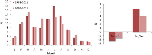
Figure 2 reveals the uneven temporal distribution of human-caused wildfires at both a monthly and a daily scale for two different time spans: 1988–2011 and 2008–2011. The monthly distribution shows a bimodal pattern with peaks in March and July, highly conditioned by the seasonality of human behaviour (winter) and weather conditions (summer). The daily distribution presents an acute deviation from a hypothetical even distribution (biased towards weekends), again revealing a differential temporal pattern in human-caused wildfire ignitions.

Figure 2. Left: Monthly distribution of human-caused wildfire. Right: Deviation (%) from even daily distribution.

According to the preliminary evidence of dissimilar intra-annual behaviour at different temporal scales, eight scenarios were created. First, we defined seasonal models, distinguishing winter (December, January and February), spring (March, April and May), summer (June, July and August) and fall (September, October and November) seasons. Additionally, working days (WD; Monday to Friday) were separated from non-working days (NWD), essentially weekends (Saturday and Sunday) and bank holidays. This led to eight intra-annual scenarios (Table 2).

Table 2. Temporal scenarios.

	Name	Description
1	WIN_WD	Working days of winter
2	WIN_NWD	Non-working days of winter
3	SPR_WD	Working days of spring
4	SPR_NWD	Non-working days of spring
5	SUM_WD	Working days of summer
6	SUM_NWD	Non-working days of summer
7	FALL_WD	Working days of fall
8	FALL_NWD	Non-working days of fall

2.5. Model calibration

2.5.1. Dependent variable

The dependent variable was constructed with wildfire data from the EGIF database (see Section 2.3). Consequently, it accounts for true cases of wildfire occurrence. As we are exploring eight scenarios of occurrence data, we split the fire events accordingly. Thus, we obtain a final set of eight subsets that make up the dependent variable across scenarios. Bearing in mind that background or ‘no occurrence’ cases are not a requirement for MaxEnt, our dependent variables only consisted of presence locations.

2.5.2. Independent variables

A set of explanatory variables was selected according to author experience (Chuvieco et al. 2014; Rodrigues et al. 2014, 2016; Rodrigues and de la Riva, 2014a, 2014b) and on other models at regional and national scales (Martínez et al. 2009; Chuvieco et al. 2010; Padilla and Vega-Garcıa 2011; Costafreda-Aumedes et al. 2017, 2018), on the basis of variable performance, and according to their relationship with wildfire ignition factors (Leone et al. 2003, 2009).

Factors related to socioeconomic changes. Human presence, population increase and urban growth. Greater pressure on wildlands.

1. Wildland-Urban Interface (WUI). Distance in metres to the intersection between any kind of natural vegetation susceptible to ignition (codes 31X and 32X) and an urban-industrial-construction area (codes 111, 112 and 121). Data was extracted from Corine Land Cover (CLC) 2006.

Factors related to traditional economic activities in rural areas. Use of fire to eliminate harvesting wastes and to clean cropland borders. These procedures are a potential source of ignition due to spread of fire to forest areas in the vicinity.

• 2. Wildland-Agricultural Interface (WAI). Distance in metres to the intersection between any kind of natural vegetation susceptible to ignition (codes 31X and 32X) and an agricultural and/or livestock area (codes 2XX). Data were extracted from 2006 CLC.

Factors which could cause fire mainly by accident or negligence. Possible cause of ignition by accident and increased human pressure on wildland.

• 3. Power lines (PWL). Distance in metres to the power line network obtained from the national cartographic database 1:25,000 (BCN25).

• 4. Roads (ROADS). Distance in metres to the road network obtained from the BCN25

• 5. Tracks (TRACKS). Distance in metres to the forestry track network obtained from the BCN25.

Factors which could hamper fires. Increasing concern about forest protection.

• 6. Protected areas (PROT_A). Categorical variable (0 = Not protected areas/1 = protected areas) obtained from obtained from the BCN25. The expected relationship to fire ignition is negative.

Fuel conditions. Finally, one MODIS product was included to determine a fair approximation of the temperature of the fuel, therefore including additional temporal variability beyond the selected temporal scenarios (Chowdhury and Hassan 2013). In this sense, we understand that the temperature of the fuel complements the influence of human activities favouring or determining if an accident or negligence leads to an actual wildfire (i.e. ignites and propagates). We are fully aware that several works use other remote sensing products such as NDVI, MOD16 or derived indexes to address Dead and Live fuel moisture content (Chuvieco et al. 2014; Chowdhury and Hassan 2015). We explored some of them and decided to employ MOD11A2 because of the temporal resolution of the product and its performance in the models.

• 7. MODIS/Terra Land Surface Temperature and Emissivity (MOD11A2 – LST). This MODIS product offers 1 km² of spatial resolution and eight-day temporal resolution. The seasonal averages were computed aggregating the monthly products of the period of study (LST_WIN, LST_SPR, LST_SUM and LST_FALL).

All variables were spatialized in raster format with a spatial resolution of 250 × 250 metres. LST products were resampled using a Nearest Neighbor approach to keep the original values (Table 3). To ensure consistency of results, we conducted an analysis of collinearity in the explanatory variables using the non-parametric Spearman’s Rho correlation index. No collinear variables were found except between LST variables, which is not a concern as these variables did not enter the model at the same time (Table 4). Supplemental material contains maps of the independent variables.

Table 3. Descriptive statistics of independent variables.

	Mean	SD	Min	Max
WUI	5041.4	3986.2	0.0	25,947.1
WAI	1609.3	2617.0	0.0	23,384.0
PWL	3873.3	3820.4	0.0	29,344.9
ROADS	1464.9	1470.7	0.0	10,636.0
TRACKS	479.3	538.5	0.0	8602.3
LST_WIN	14,025.7	175.7	13,132.5	14,372.4
LST_SPR	14,663.2	231.0	13,551.9	15,156.8
LST_SUM	15,020.3	247.2	13,897.7	15,543.5
LST_FALL	14,563.4	173.5	13,683.2	14,911.2

Table 4. Results from the collinearity analysis. Spearman’s Rho rank correlation index.

	PWL	WAI	WUI	TRACKS	ROADS	PROT_A	LST_FALL	LST_SUM	LST_SPR	LST_WIN
PWL	1.000	–0.003	0.315	0.005	0.122	0.028	–0.118	0.118	–0.064	–0.262
WAI	–0.003	1.000	0.224	–0.002	0.025	0.040	0.186	0.132	0.148	0.086
WUI	0.315	0.224	1.000	0.140	0.227	–0.002	–0.026	0.292	0.038	–0.266
TRACKS	0.005	–0.002	0.140	1.000	0.045	–0.035	0.022	0.091	0.036	–0.049
ROADS	0.122	0.025	0.227	0.045	1.000	0.062	–0.055	–0.019	–0.077	–0.041
PROT_A	0.028	0.040	–0.002	–0.035	0.062	1.000	–0.084	–0.155	–0.103	–0.027
LST_FALL	–0.118	0.186	–0.026	0.022	–0.055	–0.084	1.000	0.705	0.766	0.673
LST_SUM	0.118	0.132	0.292	0.091	–0.019	–0.155	0.705	1.000	0.724	0.131
LST_SPR	–0.064	0.148	0.038	0.036	–0.077	–0.103	0.766	0.724	1.000	0.598
LST_WIN	–0.262	0.086	–0.266	–0.049	–0.041	–0.027	0.673	0.131	0.598	1.000

2.5.3. Model development

Once the dependent and independent variables were obtained, we were able to calibrate our models for each temporal scenario. The workflow followed is summarized in Figure 3. As already stated, we did not expect the same behaviour among driving factors in the different scenarios/models since both human activities and fuel conditions are subject to temporal variation. Therefore, we ran a trial calibration in MaxEnt to check the potential contribution of our predictors. This allowed testing their relative contribution to each model, thus keeping for the final models only those variables whose combined performance explained up to 95% of the variance (Table 5). We thought the remaining variables were not representative enough and that they might add noise or unnecessary complexity.

Figure 3. Workflow followed for temporal ignition danger model.

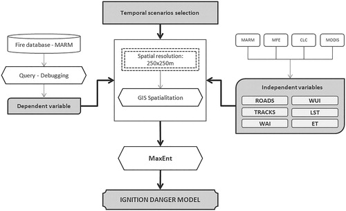
Table 5. Contribution of independent variables. grey shade indicates selected variables (up to 95% of combined explanatory power).

% contribution	WIN_WD	SPR_WD	SUM_WD	FALL_WD	WIN_WH	SPR_WH	SUM_WH	FALL_WH
ROADS	35.2	36.7	40.8	29.6	32.2	34.5	37.7	44.9
WAI	31.4	19.7	30	24.7	28.9	32.7	19.7	23
LST	13.6	24.7	9.9	17.7	15.7	23.2	13.3	10.6
WUI	10.8	3.6	10.8	19.7	9.6	5.4	13.6	16.7
PWL	6.3	14.3	6	5.1	13.4	3.3	13.5	4.3
TRACKS	1.5	0.9	1.5	3.2	0.1	0.7	1.1	0.4
PROT_A	1.1	0	1	0	0	0.2	1.1	0

2.6. Model validation and performance

Two processes for model validation were conducted. First, a model validation procedure was carried out ‘internally’ using MaxEnt software. This process was based on a cross-validation by bootstrapping and subsampling the dependent variable. Additionally, an operational validation based on a wildfire ignition probability simulation for 2012 was conducted.

Both validation procedures were quantified according to the Area Under the Receiver Operating Characteristic (ROC) curve (AUC) to evaluate model performance (Hanley and McNeil 1982). The ROC curve is a graphical representation of the false-positive error (1 - specificity, where specificity is the proportion of incorrect predictions) versus the true positive rate (also known as sensitivity or the proportion of correct predictions) for a binary classifier system and for different values of the discrimination threshold (Zhou et al. 2009). The AUC is a threshold-independent metric because it evaluates the performance of a model at all possible threshold values by adding up the area between the ROC and the random performance line (Franklin 2010). AUC values ranged from 0.5 to 1, where 0.5 is analogous to a completely random prediction (random performance line) and 1 implies perfect prediction. AUC values between 0.5 and 0.7 denote poor to low performance, values between 0.7 and 0.9 denote moderately good performance and values larger than 0.9 denote excellent model performance (McCune et al. 2002).

2.6.1. Model validation and variable contribution

We used a k-fold (k = 4) cross validation to estimate errors around fitted functions and predictive performance of models. Thus, MaxEnt randomly withheld 25% of the occurrence points for testing. AUC values were then calculated for each fold and scenario model. Therefore, four AUC values are obtained for each model.

In addition, the final contribution of each explanatory variable was estimated from a jack-knife procedure similar to Bar Massada et al. (2013). The foundation of this method relies on the fact that a binary classification system can be used to calculate ROC curves and to determine the precision of a diagnostic test (Ordóñez et al. 2012). By measuring the AUC changes to the inclusion of each variable, MaxEnt is thereby able to estimate the percentage of contribution of each variable to the model. This method is therefore valid to estimate the importance and sensitivity of the model to the unique information of each variable and compare the influence of the variables in the different temporal scenarios.

2.6.2. Operational validation

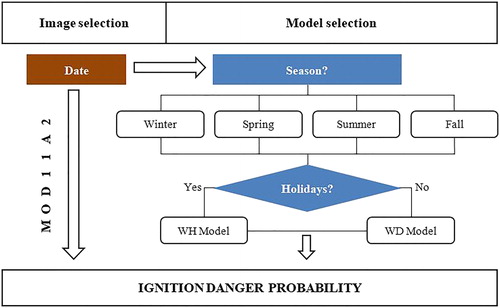
Wildfire data from 2012 were used to conduct an operational validation and testing of the predictive performance of our models. Essentially, this process is a simulation of ignition prediction at a daily scale, updating the LST layer (note that this is an eight-day temporal resolution product) and using the matching scenario. The workflow for the generation of our dynamic ignition probability approach is found in Figure 4.

Figure 4. Workflow for the dynamic prediction of wildfire ignition probability.

For in-depth validation purposes and to ascertain whether the predictions based on our dynamic approach would outperform static and semi-static approaches we compared the performance of the three solutions. The semi-static approach considers a single model (neither season nor day-type differentiation) with the updated LST product for each day. The traditional static approach was constructed without taking into consideration seasons or day-type (i.e. without temporal scenarios) and with an annual average of the LST product. This comparison will allow us to determine whether the effort of developing dynamic models is worthwhile (predictions are improved) or if semi-static models such as Chuvieco et al. (2014) perform adequately enough.

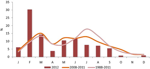
It is worth noting the special characteristics of 2012. This year is particularly interesting as a control/validation sample as it shows a slightly different intra-annual distribution when compared to the average pattern, with the peak occurrence during February (Figure 5). In addition, an extraordinary heat wave episode took place during the early fall (AEMET 2012).

Figure 5. Monthly distribution of human-caused wildfire in 2012, 2008–2011 and 1988–2011.

To evaluate the predictive performance of each approach we have calculated the AUC and constructed several boxplots to compare the predicted probability of ignition in occurrence and pseudo-absence location. AUC was evaluated separately for each season and for the entire year whereas boxplots were built per each month.

To do so, we constructed four random pseudo-background samples, creating pseudo-absence points mirroring the temporal distribution of fire occurrence observed in 2012. In other words, for each day of 2012 we created four samples of random points equal to the amount of wildfire events triggered that day, thereby obtaining four background samples (folds) matching the total amount and temporal distribution of the actual observed occurrence. The AUC was then calculated for each combination of actual fire events during 2012 and pseudo-background sample.

The operational validation was carried out using the R environment so that the entire process can be automated. The maxent package (which is an adaptation of the MaxEnt software) was used to replicate the models for each scenario.

3. Results

3.1. Variable contribution to the predicted models

Overall, as shown in Figure 6, ROADS was appreciably the most important variable in all the models with percentages ranging from 49.5% in FALL_NWD to 33.2% in SUM_WD. WAI performed as the second contributor in five models while WUI held a differential contribution across the year. LST maintained a moderate contribution in all the models. Finally, the importance of PWL was residual in most of the models, only above 10% in two of them. The AUC values presented in Table 6 support this overview, although introducing some important nuances. For instance, although the explanatory capacity of LST performing by itself is the weakest one among the variables, without its participation the models lose considerable predictive performance. Also, even though there is a relatively high contribution percentage of WAI, the models suffer the least when excluding WAI from the prediction.

Figure 6. Independent variable contributions.

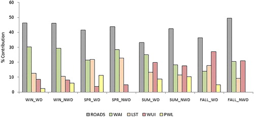
Table 6. AUC values of models with and without the participation of independent variables.

		Lost of AUC without					AUC with only
	Mean AUC	LST	ROADS	WAI	WUI	PWL	LST	ROADS	WAI	WUI	PWL
WIN_WD	0.815	–0.015	–0.017	–0.003	–0.004	0.001	0.691	0.778	0.712	0.732	0.709
WIN_WH	0.835	–0.010	–0.029	–0.004	0.001	–0.005	0.691	0.794	0.708	0.750	0.734
SPR_WD	0.843	–0.029	–0.019	–0.003	–0.002	–0.009	0.713	0.781	0.709	0.719	0.739
SPR_WH	0.852	–0.032	–0.029	–0.007	–0.006	–	0.724	0.791	0.701	0.727	–
SUM_WD	0.853	–0.016	–0.018	–0.003	–0.011	–0.005	0.681	0.791	0.727	0.761	0.751
SUM_WH	0.860	–0.013	–0.023	–0.003	–0.014	–0.005	0.679	0.805	0.713	0.753	0.762
FALL_WD	0.840	–0.018	–0.019	–0.001	–0.010	–0.001	0.704	0.782	0.693	0.766	0.741
FALL_WH	0.859	–0.007	–0.041	–0.002	–0.018	–	0.677	0.816	0.705	0.773	–
Mean	0.844	–0.017	–0.024	–0.003	–0.008	–0.004	0.695	0.792	0.709	0.748	0.739

Taking a coarse look at the different scenarios, we observe a fairly similar distribution of the variables in the winter models, with a strong importance of the ROADS followed by the WAI, reaching together around 75% of contribution to the models. In SPR_WD and SPR_NWD the importance of ROADS slightly decreases in favour of LST, which performs a key role during the spring. ROADS importance during the summer continues elevated, although it does not reach winter values, especially in working days. Summer and fall scenarios share a moderate importance of the WUI. PWL influence seems to be more relevant during the warmest scenarios, although it did not enter the models in SPR_NWD and FALL_NWD.

3.2. Model performance

Table 7 presents AUC results of the models. According to AUC values, the highest prediction capacity is reached in the summer, especially during non-working days (0.860), while the lowest is found during winter working days (0.815). However, the overall performance of the models is moderately good, according to the accuracy thresholds proposed by McCune et al. (2002). The operative validation conducted with wildfire data from 2012 confirmed the high prediction capacity of the dynamic approach, with an excellent prediction during summer and winter months and performing significantly better than the semi-static and the static approach (Table 8). The differences were especially considerable during winter and summer, when the dynamic models reached an excellent prediction capacity. The semi-static approach poorly explained the wildfire distribution during the winter, although it performed better than the static during the summer and the fall.

Table 7. AUC values of models computed in MaxEnt.

	Test AUC (min)	Test AUC (max)	Test AUC (mean)	AUC StdDev (mean)
WIN_WD	0.770	0.834	0.815	0.020
WIN_WH	0.813	0.849	0.835	0.024
SPR_WD	0.829	0.850	0.843	0.012
SPR_WH	0.837	0.870	0.852	0.014
SUM_WD	0.833	0.867	0.853	0.012
SUM_WH	0.835	0.877	0.860	0.019
FALL_WD	0.824	0.866	0.840	0.021
FALL_WH	0.848	0.875	0.859	0.031

Table 8. AUC values of models from operational validation with 2012 wildfire data.

	AUC (mean)
	WIN	SPR	SUM	FALL	Year
Dynamic approach	0.89	0.83	0.92	0.84	0.85
Semi-static approach	0.65	0.77	0.82	0.81	0.70
Static-approach	0.79	0.79	0.80	0.76	0.79

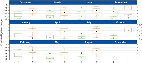
The satisfactory performance of the dynamic models is easily appreciable in Figure 7. The boxplots show how the predicted ignition probability is significantly higher for the actual location of wildfires during 2012 than for the random samples. February and March, the months with the highest number of wildfires that year, confirm this assumption, as the actual ignitions are placed in areas with a moderate-high ignition probability whereas the random sample was found, in average, in low probability areas. This pattern is similar throughout the year. September, a month abnormally warm in 2012 in the study area (AEMET 2012), shows increased values of probability. However, true cases of wildfires are still found in more prone areas (greater ignition probability) than the random samples. The lowest prediction capacity of the dynamic models is found in May, where the difference between random sample and the occurrences is the shortest.

Figure 7. Boxplot of predicted ignition probability for wildfires in 2012 (1-orange) and a random absence sample (0-green).

3.3. Spatial distribution of occurrence probability

Figures 8–11 display the logistic output for the eight temporal scenarios, with probability values ranging from 0 (null ignition risk) to 1 (maximum ignition risk), along with the uncertainty of each model, measured by the coefficient of variation (standard deviation of the 4-folds divided by the average). For representation purposes and in order to reduce the amount of output maps and to allow a comprehensive interpretation we mapped at the same time the ignition probability and the uncertainty – bivariate mapping. For this purpose, we resampled (bilinear interpolation) the cell size of the rasters to 5000 m. Then, we vectorized the outputs to obtain a point shapefile and mapped the ignition probability using a colour scheme and uncertainty using size. We must note that the size scale is inverted to represent locations with low uncertainty with larger symbols and vice versa.

Figure 8. Ignition probability and uncertainty of winter working days and non-working days. Source: National (Spain) Geographic Institute.

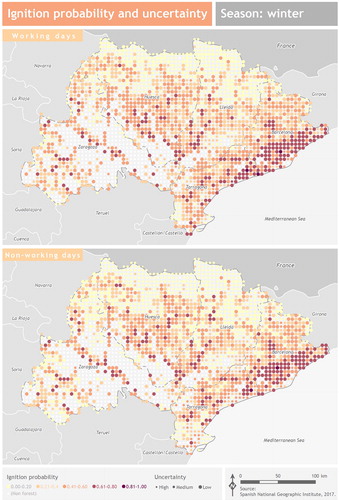
Figure 9. Ignition probability and uncertainty of spring working days and non-working days. Source: National (Spain) Geographic Institute.

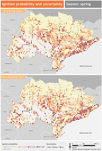
Figure 10. Ignition probability and uncertainty of summer working days and non-working days. Source: National (Spain) Geographic Institute.

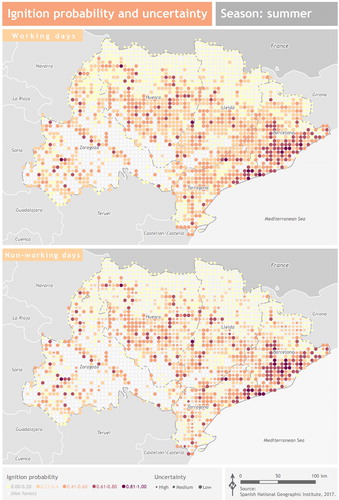
Figure 11. Ignition probability and uncertainty of fall working days and non-working days. Source: National (Spain) Geographic Institute.

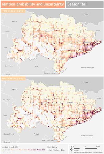
In a general overview we can observe the highest ignition probability over the easternmost portion of the area of study (i.e. the Mediterranean coast) and the south and east of the province of Huesca. Lowly populated areas such as the Pyrenees (north of Huesca and Lérida) or the Iberian range (south of Zaragoza) present the lowest probability. Overall, the areas with largest uncertainty coincide with low probability values while the uncertainty of areas with moderate or high ignition probability is limited. Due to the resampling and the fact that these are averaged models (LST of the season) do not reflect a large spatial variability and the patterns of high/low probabilities are roughly similar. The main difference is when comparing opposed seasons (winter versus summer). The moderate probability values during the winter scenarios appear more spread than during the summer, where fewer locations have moderate probability but there are more high probability areas (>0.8). In order to fully appreciate the differences that the models – along with the updating of the LST product – induce we recommend visiting the following link for an animated recreation of the 2012 wildfire season and the dynamic prediction: http://geoonline.es/simulation2012/.

4. Discussion

Modelling ignition probability by means of temporal scenarios enhances our understanding of anthropogenic drivers and, potentially, wildfire prevention. The proposed approach also improves prediction over traditional approaches. Our proposal clearly outperforms those approaches based on ‘yearly’ models (i.e. considering the occurrence as a whole and disregarding intrannual variability). For instance, Rodrigues and de la Riva (2014a, 2014b) reported AUC values around 0.74, using historical fire data in the period 1988–2007, validating their Random Forest approach with fire records from 2008 to 2011. To some extent, existing operational models such as Chuvieco et al. (2014) or Padilla and Vega-García (2011) reported satisfactory results. They propose a daily fire danger ignition framework using data from 2002 to 2004, validating with 2005. Their method is based on fitting several models, splitting the study region (mainland Spain) into 53 homogeneous ecoregions reporting AUC values ranging from 0.52 to 0.78. It should be noted that Chuvieco et al. (2014) do not report specific figures of fire ignition probability but went far beyond our approach, developing a full framework for forest fire risk modelling, combining ignition, propagation and vulnerability using what we refer to as a semi-static approach. They considered variability in fuel conditions mostly for ignition and propagation but did not account for variation in causal agents (neither natural nor human). In any case, the reported performance of these models is clearly below that from our dynamic proposal (AUCs of 0.78 in the best-case scenario in Padilla and Vega-García (2011) compared to 0.85 from our approach). Thus, we believe this kind of framework would benefit from scenario definition, at least separating the winter season from summer. From an operational perspective, the simulation of 2012 reveals how the proposed approach provides fair predictions (0.85 of yearly AUC in the dynamic simulation compared to 0.79 or 0.70 in semi-static and static approaches, respectively). Furthermore, the simulation displays acute temporal changes between seasons and days (working vs. non-working). In addition, the method highlights anomalous behaviours such as the impact of an extreme heat wave during the last week of September and the first of October. This is quite important when it comes to wildfire management since we can detect extreme conditions or at least uncommon situations of increased ignition probability. Moreover, low ignition likelihood is predicted during November, which in fact did not experience any fire.

Accessibility variables such as ROADS have been confirmed as the key factor to explain ignition probability in the area of study, which agrees with previous studies in the region (e.g. Garcia et al. 1995; Vasconcelos et al. 2001; Padilla and Vega-García 2011; Costafreda-Aumedes et al. 2018). Just like these studies, the distance to the road network is inversely related with the ignition probability – the closer to the road network, the higher the probability. Roads vicinity is a potential cause of accidents and increases the likelihood of either arson or negligence. ROADS is consistently the highest contributor to the models throughout the year. However, it shows a differential behaviour in the WD-NWD models. As we observed in Figure 6, the contribution of ROADS during weekends and holidays is notably higher compared to the working days of the same season scenario. This can be explained by the traffic increase experienced during weekends and holidays, as people tend to travel more frequently during these days, and especially in forested environments. The difference is especially relevant during the summer and fall models, which may be related to the enjoyable weather and long daytimes of the summer and with the beauty of the landscape, as well as activities such as mushroom or wild fruit picking, during the fall (Tardío et al. 2006; Martínez de Aragón et al. 2011). The second-most important variable in the models is the wildland-agricultural interface. WAI is also inversely related to the ignition risk. This pattern has also been identified in the literature (Costafreda-Aumedes et al. 2017). Rodrigues et al. (2014) highlighted the importance of this variable in the Spanish context and linked it to the synergy between agricultural and forestry activities, which often use fire for clearing forest and pasture establishment. Additionally, practices such as stubble or weeds burning or the use of fire burners as a frost-protection method are behind accidental or negligent fire ignitions (Martínez et al. 2009). Law and regulatory enforcement for these practices is strict during the wildfire high-risk season, which in Spain often starts in March and extends until the end of October. This might explain the higher importance of the WAI variable during the winter scenarios. The relatively high importance in SUM_WD might be related to the harvesting period and the likelihood of accidents involving harvest machinery (Calderón Cortés and Mateo Fernández 2017) which is frequently very old and prone to accidental sparks (MAPA 2006). The distance to the wildland-urban interface also presents an inverse relationship with fire ignition probability and its importance has been extensively discussed in the literature (e.g. Syphard et al. 2007; Chuvieco et al. 2010). Urban sprawl has been a dynamic process, especially in the Mediterranean coast during the 2000’s, which contributes to a closer contact with forested areas and therefore increases wildfire probability. WUI finds its maximum contributions to the models during the fall, followed by the summer scenarios. Again, this coincides with the time of highest recreation activity in natural areas and with the driest period of the year for Mediterranean ecosystems, which can lead to accidental or negligent ignitions. Land surface temperature was used as an ignition susceptibility variable of the fuel, following studies such as Guangmeng and Mei 2004 and Chaparro et al. 2016. The relation with the models is positive, meaning that the higher the land surface temperature is, the more likely is a fire to occur. LST shows a higher contribution during transition seasons (spring and fall), where the status of the fuel may have a greater influence over the likelihood of ignition in comparison with the winter scenarios – where the natural conditions for ignition are often not favourable – and the summer – where conditions are mostly favourable. Finally, the distance to power lines, with a negative relationship to ignition probabilities, has an overall low contribution along the models. However, it seems to be more important when the environment and atmospheric circumstances might be conducive to the occurrence of an accidental or negligent ignition, namely the summer scenarios.

From a spatial standpoint, we observe a similar pattern of ignition probability across scenarios (Figures 8–11) with an increased chance of ignition in highly populated areas such as the metropolitan area of Barcelona along the Mediterranean and the vicinity of Zaragoza in the Ebro basin, decreasing in rural settlements. The increased accessibility (ROADS) and urban sprawl (WUI) are behind the underlying spatial pattern. From a spatiotemporal perspective, the influence of WAI is noteworthy during winter scenarios, adding a ‘spray’ effect which extends areas in danger. This coincides with the notion of winter wildfires in Spain being traditionally related to agricultural activities (Martínez et al. 2009). Fire has typically been the preferred tool to eliminate stubble, weeds, field margins, hedges and shrubs. Increased agricultural activity promoted by mechanization over time, or the need to prune and burn stubble and agricultural residues, only allowed during winter months, might be behind the augmented contribution of WAI to winter fire occurrence (Martínez et al. 2009).

5. Conclusions

The consideration of the temporal dimension in modelling the human ignition probability is a step forward towards the creation of more accurate and dynamic forecasts. By integrating the temporal cycles that drive human activity within wildfire ignition probability models we overcome and outperform traditional prediction approaches that only took into consideration the temporality of the environmental factors. The methodology developed in this work and based on the Maximum Entropy algorithm has allowed evaluating the performance of the different temporal scenarios as well as the contribution of the explanatory variables in the different models. The k-fold cross-validation reported AUC around 0.85, which stands close to an excellent performance. This was confirmed by the operational validation with 2012 wildfire data. This validation also confirmed the improvement that the created dynamic models offer by comparing their performance with semi-static and static approaches. Overall, this work evidences the opportunity of improving our wildfire forecasts and reducing the risk of these hazards. From a management perspective, our proposal brings in new possibilities in terms of pre-planning by considering short-term fluctuations not only in fuel conditions, but in human activities (working vs. non-working days). This is particularly interesting during winter months, when burning and cleansing permits are usually granted.

However, we believe more research is needed, potentially extending both the spatial and the temporal scope of the project. Additionally, as technology improves and more products become available we see potential enhancements in improving the spatial resolution to fully harness the accuracy of GPS at georeferencing the location of ignitions. Finally, the inclusion of more robust variables or indexes for modelling the environmental factors could also improve the performance of the forecasts presented here.

Disclosure statement

No potential conflict of interest was reported by the authors.

Additional information

Funding

This research was funded jointly from a predoctoral Fulbright-Iberdrola grant, a ‘Juan de la Cierva’ postdoctoral fellowship grant (FJCI-2016-31090) at the Univesity of Lleida, and the research group GEOT, from the University of Zaragoza.

References

- Abbott KN, Leblon B, Staples GC, Maclean DA, Alexander ME. 2007. Fire danger monitoring using RADARSAT‐1 over northern boreal forests. Int J Remote Sens. 28(6):1317–1338. https://doi.org/10.1080/01431160600904956
- Agencia Estatal de Meteorología (AEMET). 2012. Informe mensual climatológico. Octubre de 2012. Available at:http://www.aemet.es/documentos/es/serviciosclimaticos/vigilancia_clima/resumenes_climat/mensuales/2012/res_mens_clim_2012_10.pdf
- Allgöwer B, Carlson JD, van Wagtendonk JW. 2003. Introduction to fire danger rating and remote sensing — will remote sensing enhance wildland fire danger rating? In: Chuvieco E, editor. Wildland fire danger estimation and mapping. The role of remote sensing data. Singapore: World Scientific Publishing; pp. 1–19. https://doi.org/10.1142/9789812791177_0001
- Amatulli G, Rodrigues MJ, Trombetti M, Lovreglio R. 2006. Assessing long-term fire risk at local scale by means of decision tree technique. J Geophys Res Biogeosci. 111:G04S05. https://doi.org/10.1029/2005JG000133
- Archibald S, Lehmann CER, Gomez-Dans JL, Bradstock RA. 2013. Defining pyromes and global syndromes of fire regimes. Proc Natl Acad Sci USA. 110(16):6442–6447. https://doi.org/10.1073/pnas.1211466110
- Bar Massada A, Syphard AD, Stewart SI, Radeloff VC. 2013. Wildfire ignition-distribution modelling: a comparative study in the Huron? Manistee National Forest, Michigan, USA. Int J Wildland Fire. 22(2):174. https://doi.org/10.1071/WF11178
- Calderón Cortés D, Mateo Fernández JF. 2017. Prevención de incendios en labores de recolección de cereal en Castilla-La Mancha. 7° Congreso Forestal Español. Gestion del monte: servicios ambientales y bioeconomía. Available at: http://7cfe.congresoforestal.es/sites/default/files/actas/7CFE01-439.pdf.
- Carmona A, González ME, Nahuelhual L, Silva J. 2012. Spatio-temporal effects of human drivers on fire danger in Mediterranean Chile. Bosque (Valdivia). 33(3):31–32. https://doi.org/10.4067/S0717-92002012000300016
- Chaparro D, Piles M, Vall-Llossera M, Camps A. 2016. Surface moisture and temperature trends anticipate drought conditions linked to wildfire activity in the Iberian Peninsula. Eur J Remote Sens. 49(1):955–971. https://doi.org/10.5721/EuJRS20164950
- Chelli S, Maponi P, Campetella G, Monteverde P, Foglia M, Paris E, Lolis A, Panagopoulos T. 2015. Adaptation of the Canadian fire weather index to Mediterranean forests. Nat Hazards. 75(2):1795–1810. https://doi.org/10.1007/s11069-014-1397-8
- Chen F, Du Y, Niu S, Zhao J. 2015. Modeling forest lightning fire occurrence in the Daxinganling mountains of Northeastern China with MAXENT. Forests. 6(12):1422–1438. https://doi.org/10.3390/f6051422
- Chowdhury EH, Hassan QK. 2013. Use of remote sensing-derived variables in developing a forest fire danger forecasting system. Nat Hazards. 67(2):321–334. https://doi.org/10.1007/s11069-013-0564-7
- Chowdhury EH, Hassan QK. 2015. Development of a new daily-scale forest fire danger forecasting system using remote sensing data. Remote Sens. 7(3):2431–2448. https://doi.org/10.3390/rs70302431
- Chuvieco E, Aguado I, Yebra M, Nieto H, Salas J, Martín MP, Vilar L, Martínez J, Martín S, Ibarra P, et al. 2010. Development of a framework for fire risk assessment using remote sensing and geographic information system technologies. Ecol Model. 221(1):46–58. https://doi.org/10.1016/j.ecolmodel.2008.11.017
- Chuvieco E, Aguado I, Jurdao S, Pettinari ML, Yebra M, Salas J, Hantson S, de la Riva J, Ibarra P, Rodrigues M, et al. 2014. Integrating geospatial information into fire risk assessment. Int J Wildland Fire. 23(5):606. https://doi.org/10.1071/WF12052
- Chuvieco E, Allgöwer B, Salas J. 2003. Integration of physical and human factors in fire danger assessment. In: Chuvieco E, editor. Wildland fire danger estimation and mapping. The role of remote sensing data. Singapore: World Scientific Publishing; pp. 197–218. https://doi.org/10.1142/9789812791177_0007
- Costafreda-Aumedes S, Comas C, Vega-Garcia C. 2017. Human-caused fire occurrence modelling in perspective: a review. Int J Wildland Fire. 26(12):983. https://doi.org/10.1071/WF17026
- Costafreda-Aumedes S, Vega-Garcia C, Comas C. 2018. Improving fire season definition by optimized temporal modelling of daily human-caused ignitions. J Environ Manage. 217:90–99.
- Elith J, Phillips SJ, Hastie T, Dudík M, Chee YE, Yates CJ. 2011. A statistical explanation of MaxEnt for ecologists. Divers Distrib. 17(1):43–57. https://doi.org/10.1111/j.1472-4642.2010.00725.x
- Food and Agriculture Organization (FAO). 2006. Fire management: voluntary guidelines. Principles and strategic actions. Fire Management Working Paper 17. Rome, Italy: FAO. Available at http://www.fao.org/docrep/pdf/009/j9255e/j9255e00.pdf
- Franklin J. 2010. Mapping species distributions. New York: Cambridge University Press.
- Garcia CV, Woodard PM, Titus SJ, Adamowicz WL, Lee BS. 1995. A logit model for predicting the daily occurrence of human caused forest-fires. Int J Wildland Fire. 5(2):101. https://doi.org/10.1071/WF9950101
- Guangmeng G, Mei Z. 2004. Using MODIS land surface temperature to evaluate forest fire risk of Northeast China. IEEE Geosci Remote Sens Lett. 1(2):98–100. https://doi.org/10.1109/LGRS.2004.826550
- Hanley JA, McNeil BJ. 1982. The meaning and use of the area under a receiver operating characteristic (ROC) curve. Radiology. 143(1):29–36.
- Jolly WM, Cochrane MA, Freeborn PH, Holden ZA, Brown TJ, Williamson GJ, Bowman DMJS. 2015. Climate-induced variations in global wildfire danger from 1979 to 2013. Nat. Commun. 6:7537. https://doi.org/10.1038/ncomms8537
- Koutsias N, Allgöwer B, Kalabokidis K, Mallinis G, Balatsos P, Goldammer J. 2016. Fire occurrence zoning from local to global scale in the European Mediterranean basin: implications for multi-scale fire management and policy. iForest. 9(2):195–204. https://doi.org/10.3832/ifor1513-008
- Leone V, Koutsias N, Martínez J, Vega-García C, Allgöwer B, Lovreglio R. 2003. The human factor in fire danger assessment. In: Chuvieco E, editor. Wildland fire danger estimation and mapping. The role of remote sensing data. Singapore: World Scientific Publishing; pp. 143–196.
- Leone V, Lovreglio R, Martín MP, Martínez J, Vilar L. 2009. Human factors of fire occurrence in the Mediterranean. In: Chuvieco E, editor. Earth observation of wildland fires in Mediterranean ecosystems. Berlin: Springer Berlin Heidelberg; pp. 149–170. https://doi.org/10.1007/978-3-642-01754-4_11
- Maingi JK, Henry MC. 2007. Factors influencing wildfire occurrence and distribution in eastern Kentucky, USA. Int J Wildland Fire. 16(1):23. https://doi.org/10.1071/WF06007
- Martínez J, Chuvieco E, Martín MP. 2004. Estimating human risk factors in wildland fires in Spain using logistic regression. International symposium on fire economics, planning and policy: A global vision. April 9–22; Córdoba: University of Córdoba.
- Martínez J, Vega-Garcia C, Chuvieco E. 2009. Human-caused wildfire risk rating for prevention planning in Spain. J Environ Manage. 90(2):1241–1252. https://doi.org/10.1016/j.jenvman.2008.07.005
- Martínez de Aragón J, Riera P, Giergiczny M, Colinas C. 2011. Value of wild mushroom picking as an environmental service. Forest Pol Econ. 13(6):419–424. https://doi.org/10.1016/j.forpol.2011.05.003
- Martínez-Fernández J, Chuvieco E, Koutsias N. 2013. Modelling long-term fire occurrence factors in Spain by accounting for local variations with geographically weighted regression. Nat Hazards Earth Syst Sci. 13(2):311–327. https://doi.org/10.5194/nhess-13-311-2013
- McCune B, Grace JB, Urban DL. 2002. Analysis of ecological communities. Glenden Beach: MJM Software Design.
- Ministerio de Agricultura Pesca y Alimentación (MAPA). 2006. Análisis del Parque Nacional de Tractores Agrícolas. 2005–2006. Madrid (Spain): Secretaría General de Agricultura y Alimentación. Available at: https://www.mapa.gob.es/va/agricultura/publicaciones/parque_tractores_tcm39-57883.pdf
- Ministerio de Agricultura y Pesca Alimentación y Medio Ambiente (MAPAMA). 2012. Los Incendios Forestales en España. Decenio 2001–2010. Madrid (Spain): Área de Defensa contra lncendios Forestales (ADCIF) del Ministerio de Agricultura, Alimentación y Medio Ambiente. Available at: http://www.prodetur.es/prodetur/AlfrescoFileTransferServlet?action=download&ref=a318783c-223d-4540-86ed-3837e0841679
- Moreno MV, Malamud BD, Chuvieco EA. 2011. Wildfire frequency-area statistics in Spain. Procedia Environ Sci. 7:182–187. https://doi.org/10.1016/j.proenv.2011.07.032
- National Wildfire Coordinating Group (NWCG). 2018. Glossary of wildland fire terminology. Available at: https://www.nwcg.gov/glossary/a-z.
- Ordóñez C, Saavedra A, Rodríguez-Pérez JR, Castedo-Dorado F, Covián E. 2012. Using model-based geostatistics to predict lightning-caused wildfires. Environ Model Softw. 29(1):44–50. https://doi.org/10.1016/j.envsoft.2011.10.004
- Padilla M, Vega-García C. 2011. On the comparative importance of fire danger rating indices and their integration with spatial and temporal variables for predicting daily human-caused fire occurrences in Spain. Int J Wildland Fire. 20(1):46. https://doi.org/10.1071/WF09139
- Parisien M-A, Moritz MA. 2009. Environmental controls on the distribution of wildfire at multiple spatial scales. Ecol Monogr. 79(1):127–154. https://doi.org/10.1890/07-1289.1
- Pearson RG, Raxworthy CJ, Nakamura M, Townsend Peterson A. 2007. Predicting species distributions from small numbers of occurrence records: A test case using cryptic geckos in Madagascar. J Biogeogr. 34:102–117.
- Phillips SJ, Anderson RP, Schapire RE. 2006. Maximum entropy modeling of species geographic distributions. Ecol Model. 190(3–4):231–259. https://doi.org/10.1016/j.ecolmodel.2005.03.026
- Phillips SJ, Dudík M, Schapire RE. 2004. A maximum entropy approach to species distribution modeling. Twenty-First International Conference on Machine Learning - ICML ’04. ACM Press, New York, NY; p. 83. https://doi.org/10.1145/1015330.1015412
- Renard Q, Pélissier R, Ramesh BR, Kodandapani N. 2012. Environmental susceptibility model for predicting forest fire occurrence in the Western Ghats of India. Int J Wildland Fire. 21(4):368. https://doi.org/10.1071/WF10109
- Rodrigues M, de la Riva J. 2014a. An insight into machine-learning algorithms to model human-caused wildfire occurrence. Environ Model Softw. 57:192–201. https://doi.org/10.1016/j.envsoft.2014.03.003
- Rodrigues M, de la Riva J. 2014b. Assessing the effect on fire risk modeling of the uncertainty in the location and cause of forest fires. In: Advances in forest fire research. Coimbra: Imprensa da Universidade de Coimbra; pp. 1061–1072. https://doi.org/10.14195/978-989-26-0884-6_116
- Rodrigues M, de la Riva J, Fotheringham S. 2014. Modeling the spatial variation of the explanatory factors of human-caused wildfires in Spain using geographically weighted logistic regression. Appl Geogr. 48:52–63. https://doi.org/10.1016/j.apgeog.2014.01.011
- Rodrigues M, Jiménez A, de la Riva J. 2016. Analysis of recent spatial–temporal evolution of human driving factors of wildfires in Spain. Nat Hazards. 84(3):2049–2070. https://doi.org/10.1007/s11069-016-2533-4
- Salis M, Ager AA, Finney MA, Arca B, Spano D. 2014. Analyzing spatiotemporal changes in wildfire regime and exposure across a Mediterranean fire-prone area. Nat Hazards. 71(3):1389–1418. https://doi.org/10.1007/s11069-013-0951-0
- San Miguel-Ayanz J, Carlson JD, Alexander M, Tolhurst K, Morgan G, Sneeuwjagt R, Dudley M. 2003. Current methods to assess fire danger potential. In: Chuvieco E, editor. Wildland fire danger estimation and mapping. The role of remote sensing data. Singapore: World Scientific.
- San-Miguel Ayanz J, Camia A. 2009. Forest fires at a glance: facts, figures and trends in the EU. In: Birot Y, editor. Living with wildfires: what science can tell us. A contribution to the science-policy dialogue. Joensuu, Finland: European Forest Institute; pp. 11–18.
- Sesnie SE, Gessler PE, Finegan B, Thessler S. 2008. Integrating Landsat TM and SRTM-DEM derived variables with decision trees for habitat classification and change detection in complex neotropical environments. Remote Sens Environ. 112(5):2145–2159. https://doi.org/10.1016/j.rse.2007.08.025
- Syphard AD, Clarke KC, Franklin J. 2007. Simulating fire frequency and urban growth in southern California coastal shrublands. Landscape Ecol. 22(3):431–445. https://doi.org/10.1007/s10980-006-9025-y
- Tardío J, Pardo-de-Santayana M, Morales R. 2006. Ethnobotanical review of wild edible plants in Spain. Bot J Linn Soc. 152(1):27–71. https://doi.org/10.1111/j.1095-8339.2006.00549.x
- Vasconcelos MJP, Silva S, Tomé M, Alvim M, Pereira JMC. 2001. Spatial prediction of fire ignition probabilities: comparing logistic regression and neural networks. Photogramm Eng Remote Sens. 5:101–111.
- Vélez R. 2001. Fire situation in Spain. In: Goldammer JG, Mutch RW, Pugliese P, editors. Global forest fire assessment 1990-2001. Roma: FAO.
- Verdú F, Salas J, Vega-García C. 2012. A multivariate analysis of biophysical factors and forest fires in Spain, 1991–2005. Int J Wildland Fire. 21(5):498–509.
- Vilar L, Camia A, San-Miguel-Ayanz J, Martín MP. 2016. Modeling temporal changes in human-caused wildfires in Mediterranean Europe based on land use-land cover interfaces. Forest Ecol Manage. 378:68–78. https://doi.org/10.1016/j.foreco.2016.07.020
- Vilar L, Gómez I, Martínez-Vega J, Echavarría P, Riaño D, Martín MP. 2016. Multitemporal modelling of socio-economic wildfire drivers in central Spain between the 1980s and the 2000s: comparing generalized linear models to machine learning algorithms. PLoS One. 11(8):e0161344.
- Vilar del Hoyo L, Martín Isabel MP, Martínez Vega J. 2008. Empleo de técnicas de regresión logística para la obtención de modelos de riesgo humano de incendio forestal a escala regional. Boletín de la Asociación de Geógrafos Españoles, 47(2008): 5–29.
- Zhou, X-H, McClish DK, Obuchowski NA. 2009. Statistical methods in diagnostic medicine. Vol. 569. John Wiley & Sons. Hoboken, New Jersey.
- Zumbrunnen T, Pezzatti GB, Menéndez P, Bugmann H, Bürgi M, Conedera M. 2011. Weather and human impacts on forest fires: 100 years of fire history in two climatic regions of Switzerland. Forest Ecol Manage. 261(12):2188–2199. https://doi.org/10.1016/j.foreco.2010.10.009