Assessment of post-wildfire debris flow occurrence using classifier tree

Abstract

Besides the dangers of an actively burning wildfire, a plethora of other hazardous consequences can occur afterwards. Debris flows are among the most hazardous of these, being known to cause fatalities and extensive damage to infrastructure. Although debris flows are not exclusive to fire affected areas, a wildfire can increase a location’s susceptibility by stripping its protective covers like vegetation and introducing destabilizing factors such as ash filling soil pores to increase runoff potential. Due to the associated dangers, researchers are developing statistical models to isolate susceptible locations. Existing models predominantly employ the logistic regression algorithm; however, previous studies have shown that the relationship between the predictors and response is likely better predicted using nonlinear modeling. We therefore propose the use of nonlinear C5.0 decision tree algorithm, a simple yet robust algorithm that uses inductive inference for categorical data modelling. It employs a tree-like decision making system that makes conditional statements to split data into homogeneous classes. Our results showed the C5.0 approach to produce stable and higher validation metrics in comparison to the logistic regression. A sensitivity of 81% and specificity of 78% depicts improved predictive capability and gives credence to the hypothesis that data relationships are likely nonlinear.

Keywords:

• Burn severity
• debris flow
• decision tree
• hazard assessment
• machine learning

1. Introduction

An average of 350 million hectares of land are affected annually by wildfires worldwide (van der Werf et al., 2006). There are predictions of even further increase in these occurrences with increasing trends in temperature (Westerling et al., 2006; Bond-Lamberty et al., 2007; Flannigan et al., 2009). The hazards associated with a wildfire continue even after it is contained. Its aftermath can yield itself to a spectrum of post-effects, of which debris flows are at the most disastrous end (Brock et al., 2007; Cannon et al., 2010). Debris flows are fast-moving, high-density slurry of water, sediments and debris that travels under gravity and are endued with enormous destructive power (Cannon and Gartner 2005; Cannon et al., 2010; Staley et al., 2017). They usually occur after periods of intense, short duration precipitation on steep hillslopes covered with loose erodible material (Cannon et al., 2010). They are very destructive to anything in their paths and are usually associated with fatalities. A recent event occurring on 9 January 2018 in Montecito, California resulted in 21 confirmed deaths, hundreds of injuries, and extensive damage to infrastructure including roadways, causing major freeways to be closed for days (CNN, 2018; Fox News, 2018). This debris flow event occurred following the largest fire in California’s recent past, Thomas Fire, which had been ignited a month prior and consumed a little over 280,000 acres of land.

Although debris flows are not exclusive to fire affected areas, wildfires have been known to increase the susceptibility of otherwise stable locations (Cannon et al., 2010). With the upward trend in wildfire frequencies, it is likely these events will also be on the rise. The threat of debris flow occurrence can persists for years after wildfires. A 2015 study showed that a location that experiences a wildfire event can be at risk of producing debris flows for an average of up to 2 years after the fire after which period the risk reduces due to repopulation of vegetation (DeGraff et al., 2015). A wildfire increases the susceptibility of a basin to debris flow occurrences by several mechanisms, which all work to decrease infiltration and increase the runoff generated. Some of these factors include the burning off of the rainfall intercepting vegetation (Wondzell and King, 2003; Kinner and Moody, 2008; Cannon et al., 2010), sealing of the soil pores from the generated ash (Cannon and Gartner, 2005; Larsen et al., 2009), and predominantly, the condensation of water repellent organic compounds which leave in their wake a water repellent soil that is primed for the movement of large volumes of erodible material (DeBano, 2000; Doerr et al., 2000; Cannon and Gartner, 2005; Moody and Ebel, 2012).

Accurately predicting the behavior of debris flow is decidedly difficult due to their complex physical structure, triggering mechanisms, and regional variability. There are records of studies dating as far back as the 1980s that began the onerous task of detailing the physical behavior and impact of debris flows (Hungr et al., 1984; Bovis and Jakob, 1999; Gartner et al., 2008; Cannon et al., 2010; Staley et al., 2017). With the knowledge that wildfires increase a location’s susceptibility, scientists in the past have utilized this information to develop statistical models to isolate these potentially hazardous locations. Using information on the severity of the wildfire together with other pertinent descriptors of the affected location such as basin morphology, rainfall characteristics, and soil properties have been utilized in developing these predictive models (Hungr et al., 1984; Bovis and Jakob, 1999; Gartner et al., 2008; Cannon et al., 2010; Staley et al., 2017).

Generally, there are two different approaches for predicting the likelihood of post-wildfire debris flow occurrences: deterministic (Hungr et al., 1984; Johnson et al., 1991) and probabilistic (Cannon et al., 2010; Staley et al, 2017). Researchers at the United States Geological Survey (USGS) have spearheaded work using the probabilistic approach since it provides objective results even with scanty or low-quality datasets (Hammond et al., 1992; Donovan and Santi, 2017). They have developed probability models using datasets on past debris flow events such as basin morphology, burn severity, rainfall characteristics, and soil properties to build logistic regression models that predict the statistical likelihood of post-fire debris flow occurrence in western United States (Cannon et al., 2010, Staley et al., 2013; Staley et al., 2017). This work began in 2005 but there have been several refinements to the models over the years (Cannon and Gartner 2005; Cannon et al., 2010; Staley et al., 2017). The logistic regression approach is advantageous mostly because it considers simple linear relationships which are computationally faster and easy to interpret. Up until 2017, the best available logistic regression model developed by USGS researchers for the intermountain west United States reported a sensitivity of 44% (Cannon et al., 2010) — this translates to an approximate of 4 out of 10 potential hazardous debris flow events being correctly predicted. This classifier had each of the input predictors modelled to influence the response variable independently, as such, probabilities greater than the cutoff points occurred even when the rainfall input was zero (Cannon et al., 2010). This was problematic because it is impossible for debris flows to occur in the absence of a driving high intensity, short duration rainfall (Gartner et al, 2005; Cannon et al., 2010). In a bid to improve upon this, in 2016, USGS researchers added more samples to the initial 2010 dataset to investigate if the now data-rich database could improve the initial model (Staley et al., 2016). The data size was increased from 388 samples in 2005 (Gartner et al., 2005) to 1550 samples in 2016 (Staley et al., 2016). Also, this new study introduced a link function whereby the critical inputs of the basin characteristics were multiplied by the rainfall inputs to ensure that the response probability was close to zero when there was no rainfall event. The best of these updated models had an improved sensitivity of 83% as compared to the previous 44%, with a corresponding specificity of 58% (Staley et al., 2017).

Other researchers have also looked into nonlinear probability modeling approach to investigate if more of the complex relationships between basin predictors and debris flow occurrence, which might not be discernible to linear models, can be captured with the nonlinear approach. Kern et al., 2017 explored the use of machine learning algorithms to model debris flow response. Their study explored both linear and nonlinear relationships between the predictors and response variable. They compared the accuracies offered by different linear and nonlinear models using the same dataset in Cannon et al. 2010’s study. Their results showed the nonlinear models outperformed the linear ones by as much as ∼64% giving credence to their hypothesis that the relationship between basin predictors and the debris flows occurrence might be a nonlinear one. The top model identified from the Kern et al. (2017) study was one that was built using the Naïve Bayes algorithm. This model resulted in a sensitivity of 72%, an improvement on the 44% that was initially obtained from Cannon et al., 2010’s study, and a corresponding specificity of 90% showing improved ability to predict these debris flow locations with the nonlinear model.

We are therefore proposing the application of nonlinear modeling to the 2016 dataset as well to further improve the debris flow prediction. Preliminary analyses done with the Naïve Bayes algorithm resulted in a sensitivity 75% of and a specificity of 81%, showing improved results. However, in this current study, we propose the use of the nonlinear C5.0 tree algorithm (Quinlan, 1993) as opposed to the Naïve Bayes algorithm because the Naïve Bayes model is a black box model whose inner workings are unknown. It does not offer any insight into the relationships of the predictors as they relate to the response. The C5.0 tree algorithm, was therefore chosen in particular was chosen because it is one of the simplest nonlinear algorithms with transparent outputs. It affords a nonlinear approach by identifying unique cutoffs in the different distributions of the predictors as they relate to the response. The algorithm works by splitting the data into smaller, more homogeneous groups. Stepwise decisions are made on predictors at different levels to iteratively determine unique breakpoints as they relate to the different classes of the response variable. C5.0 builds trees from a set of training data using concepts from information theory. The algorithm makes different decisions at different nodes in an attempt to sort the response variable into its homogenous classes. To determine which predictor to choose to ask which question at each node, it uses a concept called information entropy (H), a statistic measure for the average rate at which information is produced by a stochastic source of data (Shannon, 2001). Essentially, H calculates the uncertainty in any particular decision at each node. Shannon defined Η of a discrete random variable, X, with possible values (x₁, x_2,… x_n) and probability mass function P(x) as: (1) $$H=-\sum _{i=1}^{n}P\left(x_i\right){\log }_{b}P\left(x_i\right)$$(1)

where b is usually taken as base 2. For a binary response like in this project’s case, ‘no’ debris flow and ‘yes’ debris flow, the entropy distribution looks like Figure 1 below:

Figure 1. A plot of a binary entropy function showing the distribution of entropy (uncertainty) with changes in the probability of response classes. Uncertainty is lowest when the probability approaches 0 or 1, and reaches maximum when probability is 0.5.

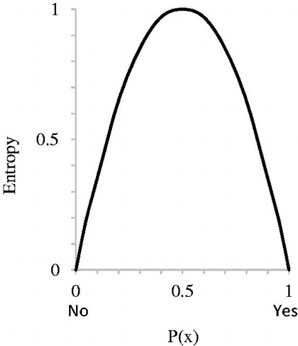
Entropy reaches a maximum at the halfway point when the probability is 0.5; i.e., there is a 50-50 chance that it could go either way (‘no’ or ‘yes’), uncertainty is at its maximum. It is lowest when the probability approaches 0 or 1. The goal is to choose the predictor which gives us the lowest entropy. Moving on from there the process is repeated for the node below; however, this time the gain, measure of entropy change, is also determined. This is to assess the magnitude of information increase in comparison to a prior node (Mitchell, 1997; Shannon, 2001). (2) $$\mathit{\text{Gain}}={\mathit{\text{Entropy}}}_{\mathit{\text{prior}}}-{\mathit{\text{Entropy}}}_{\mathit{\text{current}}}$$(2)

All candidate predictors are considered and the one with the largest information gain is chosen for the decision using a greedy system. This process is applied recursively from the root node down until a subset contains only samples of a single class, or the partitioning tree has reached a predetermined maximum depth. The C5.0 tree algorithm uses boosting in its model training process, which works by combining average model decisions together to improve overall model performance of the final output. The particular objective of this study was to investigate the applicability of the nonlinear C5.0 tree algorithm in predicting the likelihood of post-wildfire debris flow occurrences in the western U.S. and to determine if there is any advantage to be obtained over the linear logistic regression approach with this new dataset.

2. Method

2.1. Data

Data for this study were obtained from USGS’ open file report 2016-1106 (Staley et al., 2016). It comprises descriptive information on 1550 burned basins in western United States (Figure 2).

Figure 2. Map showing the 1550 burned basins considered in this study. Red dots show locations that experienced debris flows and the green dots show locations that experienced none. Source: World Terrain Base by Esri. http://downloads2.esri.com/ArcGISOnline/docs/tou_summary.pdf and https://www.arcgis.com/home/item.html?id=c61ad8ab017d49e1a82f580ee1298931

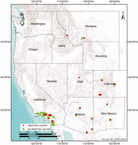
Besides the response variable, there were a total of 16 predictors, which included information on the basin morphology, burn severity, soil properties, rainfall characteristics, and other ancillary data. Brief summaries of predictors have been provided in Table 1.

Table 1. Brief descriptions of model predictors.

Predictor	Description
Acc015	Peak 15-minute rainfall accumulation of storm, in millimeters
Acc030	Peak 30-minute rainfall accumulation of storm, in millimeters
Acc060	Peak 60-minute rainfall accumulation of storm, in millimeters
Area	Contributing area of observation location, in square kilometers
dNBR	Average differenced normalized burn ratio of watershed
GaugeDist	Distance from rain gauge to documented response location, in meters
Iave	Average storm intensity, in millimeters per hour
KF	Average KF-factor a basin. Also known as the erodibility factor. It is the susceptibility of soil particle to detached and get transported by rainfall.
Peak_I15	Peak 15-minute rainfall intensity of storm, in millimeters per hour
Peak_I30	Peak 30-minute rainfall intensity of storm, in millimeters per hour
Peak_I60	Peak 60-minute rainfall intensity of storm, in millimeters per hour
PropHM23	Proportion of watershed burned at high or moderate severity and with slope >23°
Soil	Thickness of soil to the closest ‘restrictive layer’ that significantly impede the movement of water and air through the soil.
StormAccum	Total rainfall accumulation of storm, in millimeters
StormDate	Date of storm that produced the debris-flow response
StormDur	Total duration of storm, in hours

2.2. Model development

The data from Staley et al., 2016 were all given as independent predictors. As was done in Staley et al., 2017, we introduced a link function by multiplying the morphological and burn properties predictors by rainfall predictors, since debris flows cannot occur in the absence of a driving storm. A total of 35 compound predictors were obtained after this. Preliminary data pre-processing steps taken to ensure optimal model performance included omitting observations with missing values and assessing predictor degeneracy. We also observed the existence of correlations between predictors so we performed a pairwise collinearity test. The results showed that 15 predictors had 99% or more correlations with other predictors. These were regarded as redundant information and were thus deleted, leaving 20 predictors for further analyses. We run a predictor selection routine that tested the performance of candidate models with successively fewer predictors (Dillon et al., 2011; Birch et al., 2015). By this, we assessed the influence of each individual predictor on the model as a whole. We examined the variable importance from the C5.0 Tree modeling process. With each model run, C5.0 tree calculates variable importance by randomly permuting the values of each variable, one at a time, and assessing the overall improvement in the optimization criteria (accuracy, in this case). We determined the rankings of stable predictor importance by running 10 reproducible C5.0 tree models with all the 20 remaining predictors. From here, we determined a single value of importance for each predictor from the mean variable importance of all 10 candidate models and ranked them (1 = highest importance; 20 = least importance). A threshold of 50 was applied, narrowing down the predictor size to five most informative. Finally, to ensure that predictors were truly independent we performed a pairwise collinearity test once more and applied a cutoff of 60%. This resulted in these three final predictors for modelling: Soil* peakI30, PropHM23*peakI30, and KF*peakI30.

Using the final three predictors, we split the data into 70% training and 30% validation sets using stratified random sampling to ensure that representative distributions of the response variable were represented in each set, since the data were skewed towards the ‘no debris flow’ response at about 3:1. A repeated 10-fold cross validation resampling was applied to determine the number of trials needed to achieve optimal model performance. An interval of 1–30 was set as the candidates for this process. The results from the resampling were then aggregated into a performance profile which revealed optimal number of trials to be 11. Setting this as the optimum number of trials, the model was developed a final time using the entire training data.

2.3. Model evaluation

The developed model was then tested on the initial 30% validation set that was retained after preprocessing. To define the performance profile, we first generated a confusion matrix (Table 2) to summarize how the model’s predictions performed against the actual data.

Table 2. Confusion matrix.

		Predicted class
		Yes	No
Actual class	Yes	True positives (TP)	False negatives (FN)
	No	False positives (FP)	True negative (TN)

From this we determined the sensitivity (Equation (1)(1) $$H=-\sum _{i=1}^{n}P\left(x_i\right){\log }_{b}P\left(x_i\right)$$(1) ), which measures the fraction (or percentage) of debris flow producing locations that were correctly predicted by the model. This metric was given the highest priority because it gives a direct measure of the objective of the study. It runs from 0 to 1, with 1 representing a perfect model that correctly classifies all the debris flow locations. The specificity (Equation (2)(2) $$\mathit{\text{Gain}}={\mathit{\text{Entropy}}}_{\mathit{\text{prior}}}-{\mathit{\text{Entropy}}}_{\mathit{\text{current}}}$$(2) ) was also determined as the measure of the fraction (or percentage) of locations that did not produce any debris flows that were correctly predicted by the model. This metric also runs from 0 to 1, with 1 representing a perfect model that correctly classifies all the no debris flow locations. We were also interested in this metric since it assesses the model’s robustness in preventing false positives.

The third metric was the overall accuracy (Equation (3)(3) $$\mathit{\text{Sensitivity}}\mathrm{}=\mathrm{}\frac{TP}{TP+FN}$$(3) ), which measures the overall performance of the model in correctly distinguishing between debris flow and no debris flow locations. A score of 1 indicates a perfect model and 0 indicates a model with no predictive capability. Threat score (Equation (4)(4) $$\mathit{\text{Specificity}}\mathrm{}=\mathrm{}\frac{TN}{TN+FP}$$(4) ), also known as the critical success index (Schaefer, 1990), was also considered. It is another metric that measures a model’s overall performance. It is especially used when the class distributions of the response variable are as skewed toward one class, as is present in our data. This metric, however, does not consider true negative (TN) events. Cohen’s Kappa (Equation (5)(5) $$\mathit{\text{Accuracy}}\mathrm{}=\mathrm{}\frac{TP+TN}{TP+FP+TN+FN}$$(5) ), also provides a measure of the overall performance of the model by measuring the similarity between predictions and observations while correcting for agreement that occurs by chance (Cohen, 1960). The kappa statistic tends to be quite conservative but it is a more robust measure than the overall accuracy since it takes into account the possibility of chance predictions. Therefore typically, values within 0.30–0.50 on a scale of –1 to 1 indicate reasonable agreement (Kuhn and Johnson, 2013). (3) $$\mathit{\text{Sensitivity}}\mathrm{}=\mathrm{}\frac{TP}{TP+FN}$$(3)

(4) $$\mathit{\text{Specificity}}\mathrm{}=\mathrm{}\frac{TN}{TN+FP}$$(4) (5) $$\mathit{\text{Accuracy}}\mathrm{}=\mathrm{}\frac{TP+TN}{TP+FP+TN+FN}$$(5) (6) $$\mathit{\text{Threat}}\mathrm{}\mathit{\text{score}}\mathrm{}=\mathrm{}\frac{TP}{TP+FP+FN}$$(6) (7) $$\mathit{\text{Kappa}}\mathrm{}=\mathrm{}\frac{p_0-p_e}{1-p_e}$$(7)

where p₀ is the total accuracy given as: $p_0\mathrm{}=\mathrm{}\frac{TP+TN}{TP+FP+TN+FN}$, and p_e is the random accuracy given as: $p_e=\frac{\left(TN+FP\right)+\left(TN+FN\right)+\left(FN+TP\right)+\left(FP+TP\right)}{{\left(TP+FP+TN+FN\right)}^2}$

We evaluated the validation data on all these five metrics together because each of these metrics has its own biases, hence, using them together gave a better picture of the model’s performance. For example, by virtue of the skewed nature of the data, if we consider the threat score metric, it will afford us the ability to prioritize the low-frequency debris flow locations, since it ignores the TNs in its computation. However, considering this metric alone would have meant that we would not have been able to fully assess the influence of the false positives in relation to how many no-debris flow locations were present. That information is necessary to assess whether or not the model holds the risk of desensitizing the public, showing the need for considering all these metrics. To further test robustness and stability, the entire modeling process from resampling, training, and validation was repeated for ten different combinations of data samples and the best among these was selected.

3. Results and discussion

In this study, we used C5.0 decision tree algorithm to develop predictive models with the aim of isolating locations in western U.S. that will likely produce post-wildfire debris flows. Ten candidate models were built in order to investigate the robustness and stability of the algorithm. The average of validation metrics for the candidate models have been presented in Table 3. The results gave stable as well as high metrics for all 10 candidates with an average sensitivity of 77%, which is an improvement on the 66% from the logistic regression method (Table 4), thereby giving confidence in the use of the nonlinear C5.0 algorithm for our study. This algorithm was robust in distinguishing between the two classes of the response, even though the data distribution was skewed towards the ‘no debris flow’ class. The 2017 study done on this same dataset using logistic regression approach (Staley et al., 2017) reported validation outputs as TPs, TNs, FPs, and FNs hence, we have computed the corresponding sensitivities, specificities, kappas, and accuracies (Table 4), to allow for direct comparison of the two different approaches.

Table 3. Validation metrics of the 10 candidate models developed with the C5.0 tree algorithm.

Model	Validation metrics
	Accuracy	Sensitivity	Specificity	Kappa	Threat score
1	0.77	0.82	0.75	0.47	0.45
2	0.80	0.71	0.83	0.49	0.46
3	0.78	0.81	0.78	0.49	0.47
4	0.81	0.74	0.84	0.53	0.49
5	0.76	0.78	0.75	0.45	0.44
6	0.78	0.78	0.78	0.49	0.46
7	0.80	0.77	0.81	0.52	0.48
8	0.80	0.76	0.81	0.51	0.47
9	0.79	0.75	0.80	0.49	0.46
10	0.76	0.74	0.77	0.44	0.43
Average	0.79	0.77	0.79	0.49	0.46

Table 4. Validation metrics computed from the results of the logistic regression models developed by Staley et al., 2017.

Model	Validation metric
	Accuracy	Sensitivity	Specificity	Kappa	Threat Score
M1_15	0.64	0.81	0.58	0.30	0.39
M1_30	0.67	0.71	0.66	0.29	0.34
M1_60	0.73	0.46	0.81	0.26	0.27
M2_15	0.64	0.81	0.57	0.30	0.38
M2_30	0.67	0.74	0.65	0.30	0.35
M2_60	0.74	0.46	0.82	0.27	0.28
M3_15	0.60	0.84	0.52	0.26	0.36
M3_30	0.62	0.82	0.56	0.27	0.34
M3_60	0.71	0.48	0.76	0.20	0.24
M4_15	0.61	0.79	0.54	0.25	0.36
M4_30	0.61	0.67	0.58	0.20	0.31
M4_60	0.69	0.37	0.79	0.16	0.23
Average	0.66	0.66	0.65	0.26	0.32

Comparing Table 3 to Table 4, we can see that the logistic regression algorithm produces generally lower metrics than the C5.0 approach. Its highest sensitivity of 84% corresponded to a specificity of 52%, which goes with the general theme of its results, where high sensitivities corresponded to low specificities, and vice versa. In other words, the model had a harder time isolating actual debris flow locations without lumping some of the no debris flow locations (false positives) with them. This is likely due to the linear nature of the logistic regression algorithm being unable to capture much of the complex relationships to discern between little nuances as they relate to the likelihood of debris flow occurrence.

The C5.0 tree, on the other hand, affords a nonlinear approach by identifying unique cutoffs in the different distributions of the predictors as they relate to the response. Model 3 from Table 3 was chosen to be the overall best model since it had a high sensitivity with an equally high specificity, as well as a simple tree structure. A confusion matrix of the resulting classification of the test data for this model is presented in Table 5. The resulting sensitivity is 81% and the specificity is 78%, which shows an increased capacity to correctly identify ∼8 out of 10 of these hazardous debris flow locations with a very low risk (∼22%) of collating numerous false positives in the process.

Table 5. Confusion matrix of the top model using the C5.0 tree algorithm.

Actual class	Predicted class
		Yes	No
	Yes	75	18
	No	67	234

The comprehensive list of rainfall predictors investigated in this study include rainfall accumulations in 15, 30, and 60 min, respectively, peak rainfall intensities in 15, 30, and 60 min, respectively, total rainfall accumulation as well as average rainfall intensity. A look at the decision tree plot (Figure 3), however, reveals that it was only the peakI30 rainfall predictor that the model found to be most informative. This suggests that it does not take much time (at most 30 min) for a post-wildfire debris flows to be triggered once an intense storm (peak) starts, which agrees with what is found in literature (Cannon et al., 2010).

Figure 3. Graphical representation of the adopted C5.0 tree model.

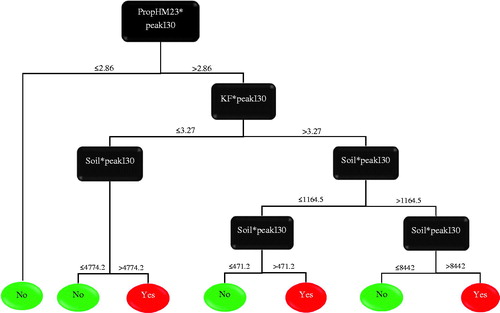
As was discussed earlier, the rainfall predictors are very essential because debris flows cannot occur in the absence of a triggering storm event. However, since the peakI30 predictor was multiplied to each of the other predictors used in the study, it will be considered as a constant in the following discussion of the tree decisions. The generated simple tree comprised a root, five branch nodes and seven leaf nodes; therefore there were seven different decision paths. The accuracy of the decisions were individually ∼60% or better. The most important predictors were the PropHM23, which indicates the proportion of moderate-high burn severity locations that have slopes that are 23% or higher, as well as the Soil predictor, which measures the overburden thickness over a ‘restrictive layer’ such as bedrock, cemented layers, frozen layers, etc. The PropHM23 was the root of the tree and thus formed the basis of every decision made, whereas the soil was the ‘tie-breaker’ for ∼86% of the decisions.

A quick overview of the seven decision nodes showed that the model was flexible enough to discourage the training data from overfitting to it. Taking the decision path from the root to leaf node 1, shows that fire affected location that are on higher elevations (slope >23%) but sustained mostly lower severity burns, i.e., lower moderate-high burn severity burn (PropHM23*peak_I₃₀ < 2.9) will likely not produce any debris flows. This decision was especially reassuring because it agrees with the main premise of this study that wildfires increase the susceptibility of a location to debris flow occurrences. A look at decisions 2 through to 7 seem to suggest that the thicker the soil overburden over a ‘restrictive layer’ (Soil*peak_I₃₀), the higher a location’s chance of generating post-wildfire debris flows. A speculation can be drawn that this is likely due to the fact that the basin will now have a greater supply of loose sediment primed for movement by a triggering rainfall. Decisions 4 and 6 further buttress this point by suggesting that even with a higher erodibility factor (KF), a basin might not be susceptible to post-fire debris flows, if it has little supply of loose material to move. In summary, the comprehensive tree seems to suggest that:

• Post-wildfire debris flows are triggered by high intensity storms that occur over short periods.

• Any location with an ample steepness in terrain (slope >23) that experiences moderate to high severity burns (PropHM23) has an increased capacity to produce debris flows.

• Coupled with this, the thicker the soil overburden over a ‘restrictive layer’, the higher the chances of generating these events.

These are in no way new discoveries as past studies have reported or alluded to them. In fact, the recent logistic regression modeling identified these similar predictors as well (Staley et al., 2017). The agreement confirms the importance of these predictors and gives rise to the recommendation to focus future studies on the cutoff points identified by the C5.0 tree algorithm. This will further our understanding of the triggering and driving forces to better prepare and mitigate future hazardous events.

4. Conclusions and future work

The main focus of this study has been to investigate the use of nonlinear C5.0 tree algorithm in predicting the likelihood of post-wildfire debris flow occurrences in the western U.S. and compare it to the results obtained from the logistic regression approach. The results showed the C5.0 approach to produce stable and higher validation metrics in comparison to the logistic regression. It had an average sensitivity of 77%, which is an improvement on the 66% from the logistic regression approach. Analyzing the resulting tree of the adopted C5.0 tree model buttressed the intuitive hypotheses that a location with a steep terrain (slope >23) that experiences moderate to high burn severity fires and laden with thick overburden soil is highly susceptible to such events. All these give rise to the conclusion that the relationship between the predictors and the response is nonlinear as opposed to the linear one offered by the logistic regression.

Disclaimer

The views, opinions, findings, and conclusions reflected in this paper are the responsibility of the authors only and do not represent the official policy or position of the USDOT/OST-R or any State or other entity.

Acknowledgments

The authors would also like to thank the following individual and institution for their contributions and roles in making this work possible: Caesar Singh, USDOT program manager and the USGS for making the data freely available online.

Disclosure statement

No potential conflict of interest was reported by the authors.

Additional information

Funding

This project was funded by the US Department of Transportation (USDOT) through the Office of the Assistant Secretary for Research and Technology,USDOT Cooperative Agreement No. OASRTRS-14-H-UARK.

References

- Birch DS, Morgan P, Kolden CA, Abatzoglou JT, Dillon GK, Hudak AT, Smith A. 2015. Vegetation, topography and daily weather influenced burn severity in central Idaho and western Montana forests. Ecosphere. 6(1):1–23.
- Bond-Lamberty B, Peckham SD, Ahl DE, Gower ST. 2007. Fire as the dominant driver of central Canadian boreal forest carbon balance. Nature. 450(7166):89–92.
- Bovis MJ, Jakob M. 1999. The role of debris supply conditions in predicting debris flow activity. Earth Surf Process Landforms. 24(11):1039–1054.
- Brock RJ, Cannon SH, Gartner J, Santi PM, Higgins JD, Bernard DR. 2007. An ordinary storm with an extraordinary response: Mapping the debris-flow response to the December 25, 2003 storm on the 2003 Old and Grand Prix fire areas in southern California. In 2007 GSA Denver Annual Meeting. Colorado: Geological Society of America.
- Cannon SH, Gartner JE. 2005. Wildfire-related debris flow from a hazards perspective. In Debris-flow hazards and related phenomena (pp. 363–385). Berlin, Heidelberg: Springer.
- Cannon SH, Gartner JE, Rupert MG, Michael JA, Rea AH, Parrett C. 2010. Predicting the probability and volume of postwildfire debris flows in the intermountain western United States. Geol Soc Am Bull. 122(1-2):127–144.
- Cohen J. 1960. A coefficient of agreement for nominal scales. Educ Psychol Meas. 20(1):37–46.
- CNN 2018. California mudslides: Death toll rises to 20, 4 still missing. January 15, 2018.
- DeBano LF. 2000. The role of fire and soil heating on water repellency in wildland environments: a review. J Hydrol. 231-232:195–206.
- DeGraff JV, Cannon SH, Gartner JE. 2015. The timing of susceptibility to post-fire debris flows in the Western United States. Environ Eng Geosci. 21(4):277–292.
- Dillon GK, Holden ZA, Morgan P, Crimmins MA, Heyerdahl EK, Luce CH. 2011. Both topography and climate affected forest and woodland burn severity in two regions of the western US, 1984 to 2006. Ecosphere. 2(12):1–33.
- Doerr SH, Shakesby RA, Walsh R. 2000. Soil water repellency: its causes, characteristics and hydro-geomorphological significance. Earth-Sci Rev. 51(1-4):33–65.
- Donovan IP, Santi PM. 2017. A probabilistic approach to post-wildfire debris-flow volume modeling. Landslides. 14(4):1345–1360.
- Flannigan MD, Krawchuk MA, de Groot WJ, Wotton BM, Gowman LM. 2009. Implications of changing climate for global wildland fire. Int J Wildland Fire. 18(5):483–507.
- Fox News 2018 February 9. California mudslides: Where and why they happen. Fox News.
- Gartner JE, Cannon SH, Bigio ER, Davis NK, Parrett C, Pierce KL, Rupert MG, Thurston BL, Trebish MJ, Garcia SP, et al. 2005. Compilation of data relating to the erosive response of 608 recently-burned basins in the western United States. No. 2005-1218. Virginia: US Geological Survey.
- Gartner JE, Cannon SH, Santi PM, Dewolfe VG. 2008. Empirical models to predict the volumes of debris flows generated by recently burned basins in the western US. Geomorphology. 96(3-4):339–354.
- Hammond CJ, Prellwitz RW, Miller SM. 1992. February. Landslide hazard assessment using Monte Carlo simulation. Proceedings of 6th International Symposium On Landslides, Christchurch, New Zealand, Balkema (Vol. 2, pp. 251–294).
- Hungr O, Morgan GC, Kellerhals R. 1984. Quantitative analysis of debris torrent hazards for design of remedial measures. Can Geotech J. 21(4):663–677.
- Johnson PA, McCuen RH, Hromadka TV. 1991. Magnitude and frequency of debris flows. J Hydrol. 123(1-2):69–82.
- Kern A, Addison P, Oommen T, Salazar S, Coffman R. 2017. Machine learning based predictive modeling of debris flow probability following wildfire in the intermountain Western United States. Math Geosci. 49(6), 717–735.
- Kinner DA, Moody JA. 2008. Infiltration and runoff measurements on steep burned hillslopes using a rainfall simulator with variable rain intensities. Virginia: U.S. Geological Survey.
- Kuhn M, Johnson K. 2013. Applied predictive modeling. New York, NY: Springer.
- Larsen IJ, MacDonald LH, Brown E, Rough D, Welsh MJ, Pietraszek JH, Libohova Z, de Dios Benavides-Solorio J, Schaffrath K. 2009. Causes of post-fire runoff & erosion: water repellency, cover, or soil sealing?. Soil Sci Soc Am J. 73(4):1393–1407.
- Mitchell TM. 1997. Machine learning. 1997. Burr Ridge, IL: McGraw Hill, 45(37), pp.870–877.
- Moody JA, Ebel BA. 2012. Hyper-dry conditions provide new insights into the cause of extreme floods after wildfire. Catena. 9358–63.
- Quinlan JR. 1993. Constructing decision tree. C4.5. San Francisco, USA : Morgan Kaufmann Publishers Inc. pp.17–26.
- Schaefer JT. 1990. The critical success index as an indicator of warning skill. Wea Forecast. 5(4):570–575.
- Shannon CE. 2001. A mathematical theory of communication. Sigmobile Mob Comput Commun Rev. 5(1):3–55.
- Staley DM, Kean JW, Cannon SH, Schmidt KM, Laber JL. 2013. Objective definition of rainfall intensity–duration thresholds for the initiation of post-fire debris flows in southern California. Landslides. 10(5):547–562.
- Staley DM, Negri JA, Kean JW, Laber JL, Tillery AC, Youberg AM. 2017. Prediction of spatially explicit rainfall intensity–duration thresholds for post-fire debris-flow generation in the western United States. Geomorphology. 278149–162.
- Staley DM, Negri JA, Kean JW, Laber JL, Tillery AC, Youberg AM. 2016. Updated logistic regression equations for the calculation of post-fire debris-flow likelihood in the western United States. Virginia: U.S. Geological Survey. No. 2016-1106.
- van der Werf GR, Randerson JT, Giglio L, Collatz GJ, Kasibhatla PS, Arellano AF. Jr, 2006. Interannual variability in global biomass burning emissions from 1997 to 2004. Atmos Chem Phys. 6(11):3423–3441.
- Westerling AL, Hidalgo HG, Cayan DR, Swetnam TW. 2006. Warming and earlier spring increase western US forest wildfire activity. Science. 313(5789):940–943.
- Wondzell SM, King JG. 2003. Postfire erosional processes in the Pacific Northwest and Rocky Mountain regions. For Ecol Manag. 178(1-2):75–87.