Positive and negative ionospheric disturbances prior to the 2016 christmas earthquake in Chile

Abstract

Global ionospheric maps (GIMs) provided by the Center for Orbit Determination in Europe (CODE) served to analyze ionospheric disturbances prior to the December 25, 2016 earthquake in Chile. Generating global two-dimensional differential vertical total electron content (VTEC) maps it was possible to detect three ionospheric disturbances. Eleven days (December 14, 2016) before the seismic event a positive ionospheric anomaly was detected. On the other hand, 8, 7 and 6 days prior to the earthquake, two negative ionospheric anomalies were also observed. All three anomalies were seen to fall inside the earthquake preparation region. Because during the days in which all three anomalies were observed, the geomagnetic and solar conditions were rather quiet and also the anomalies were localized, it can be suggested that they are seismo-ionospheric signatures due to the Chiloé earthquake. Moreover, it could be also indicated that the possible physical mechanism that originates these three anomalies is air ionization due to the emanation of radon from the Earth’s crust. It is very likely that for the negative ionospheric anomaly observed between December 18 and December 19, 2016, the fountain effect of the Equatorial Ionization Anomaly (EIA) plays a role as well in its generation.

Keywords:

• Ionospheric anomalies
• earthquakes
• vertical total electron content
• global ionospheric maps
• differential vertical total electron content maps

1. Introduction

Because of its location, atop of the subducting Nazca plate, earthquakes are constantly happening in Chile (Lomnitz 2004; Reddy et al. 2016; Ruiz and Madariaga 2018). Some of the major ones in the recent years, for instance, the September 16, 2015 Mw 8.3 (Ren et al. 2017) and the April 1, 2014 Mw 8.2 (Thorne et al. 2014) earthquakes, were the cause of many fatalities according to the media.

In an effort to look for precursors to seismic events, many studies on seismo-ionospheric signatures have been carried out (e.g. Liu et al. 2004; Zakharenkova et al. 2006, 2008; Mubarak et al. 2009; Zhu et al. 2010; Zou and Zhao 2010; Yao et al. 2012; Zhu et al. 2013; Wang et al. 2014; Xinzhi et al. 2014; Li et al. 2015; Guo et al. 2015; Pundhir et al. 2015; Alcay 2016). The methods to identify ionospheric anomalies prior to an earthquake are various. One of the most used ones (e.g. Zhou et al. 2009; Oikonomou et al. 2017), consists in looking at the time series of the Vertical Total Electron Content (VTEC) derived from Global Positioning System (GPS) data. Another widely spread technique (e.g. Zhao et al. 2008; Zhu et al. 2010, 2013; Li et al. 2015; Guo et al. 2015) consists in the analysis of two-dimensional differential VTEC (ΔVTEC) maps, which are created using Global Ionospheric Maps (GIMs). A third, well-known method, is in the case when an earthquake occurs at low-latitudes. Pulinets and Legen’ka (2002) have indicated that the Equatorial Ionization Anomaly (EIA, Appleton 1946) can undergo considerable modifications due to ionospheric anomalies. These effects were already observed prior to some low-latitude seismic events, for example, by Zakharenkova et al. (2006) and Zakharenkova et al. (2008).

Ionospheric disturbances were already detected for one of the most recent major earthquakes in Chile (Reddy et al. 2016; Daneshvar and Freund 2017). A coseismic ionospheric anomaly was detected by Reddy et al. (2016) 10 min after the Illapel earthquake in Chile of Mw 8.3 that happened on September 16, 2015. They detected this disturbance by deriving VTEC directly from GPS data. On the other hand, Daneshvar and Freund (2017) observed ionospheric anomalies 35–40 days prior to the seismic event. They achieved these detections by observing the VTEC time series, derived from GIMs, near the vicinity of the epicenter.

In this article, GIMs provided by the Center for Orbit Determination in Europe (CODE) were used in order to look for seismo-ionospheric signatures related to the 2016 Christmas earthquake that occurred in Chile.

2. The Chiloé earthquake

The Mw 7.6 earthquake, that occurred at 14:22 UT (09:00 local time; LT) on December 25, 2016 in Chile, had its epicenter (43.4°S 73.9°W) south of the Chiloé island and originated in the Earth’s crust (depth 38 km). According to Ruiz et al. (2017) and Lange et al. (2018), this subduction zone, the convergence of the Nazca and South American plates, is constantly generating seismic activity. In the recent years, a number of earthquakes of major (in this article major are considered as M ≥ 7) magnitude have happened in Chile (Figure 1). In Table 1 the major earthquakes that occurred since the beginning of 2011 in the Chilean margin are listed. Luckily for the Chiloé earthquake, no casualties were reported by the media.

Figure 1. The red circle indicates the epicenter of the Chiloé earthquake. The blue circles show the epicenters of Mw ≥ 7 earthquakes that struck the coast of Chile in the recent years (Table 1).

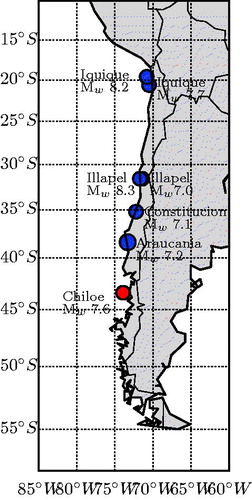
Table 1. List of M ≥ 7 earthquakes that occurred in Chile since 2011. The coordinates, the moment magnitudes and the depths were retrieved from the United States Geological Survey (USGS).

Earthquake	Coordinates	Date	Mw	Depth (km)
Chiloé	43.4°S 73.9°W	2016-12-25	7.6	38.0
Illapel	31.6°S 71.4°W	2015-09-16	7.0	28.4
Illapel	31.6°S 71.7°W	2015-09-16	8.3	22.4
Iquique	20.6°S 70.5°W	2014-04-03	7.7	22.4
Iquique	19.6°S 70.7°W	2014-04-01	8.2	25.0
Constitución	35.2°S 72.2°W	2012-03-25	7.1	40.7
Araucania	38.4°S 73.3°W	2011-01-02	7.2	24.0

3. Data analysis

3.1. Ionospheric data

IONEX files (Schaer et al. 1998), containing GIMs, were downloaded from the CODE ftp site (ftp://ftp.aiub.unibe.ch/CODE/). The retrieved files belonged to the range of days between December 9, 2016 and January 4, 2017. Each GIM consists of a 5° × 2.5° grid (longitude and latitude, respectively) of VTEC data. The units of the VTEC are given in TECU, where 1 TECU = 10¹⁶ electrons/m².

In order to identify ionospheric anomalies in the GIMs of the selected days, a sliding window of 8 days before the earthquake was used to calculate the median (X) and the interquartile range (IQR). Considering that the VTEC follows a normal distribution within the window (e.g. Liu et al. 2004; Zou and Zhao 2010; Hasbi et al. 2011; Li et al. 2015), the upper and lower bounds of the interquartile range are defined as: (1) $${\text{UB}}_{\text{IQR}}=\mu +1.34\sigma$$(1) (2) $${\text{LB}}_{\text{IQR}}=\mu +1.34\sigma$$(2) where μ is the mean and σ the standard deviation.

If the difference between the VTEC, for a certain day at a particular time, and the UB or LB is positive or negative (known also as differential VTEC; ΔVTEC), respectively, it is said that there is an ionospheric disturbance. At this point it is worth noting, that even though the accuracy of the GIMs are between 2 and 8 TECU; the tolerance of 1.34σ to define the UB and LB should make possible to detect ΔVTEC between 2 and 3 TECU, which has been indicated for instance by Ulukavak and Yalcinkaya (2017). According to the aforementioned tolerance, a positive or negative ionospheric disturbance is detected with a confidence level of 80–85%.

The UB and LB were calculated for every grid point in the GIMs. Subsequently, it was possible to construct a ΔVTEC cube, where the x and y axes are the longitude and latitude, respectively, and the z axis is the number of hours, 648 in total (between December 9, 2016 and January 4, 2017). If the ΔVTEC > UB or ΔVTEC < LB, a positive or negative ionospheric anomaly is identified, respectively. Otherwise, if UB > ΔVTEC > LB, then ΔVTEC = 0.

3.2. Geomagnetic and solar activity

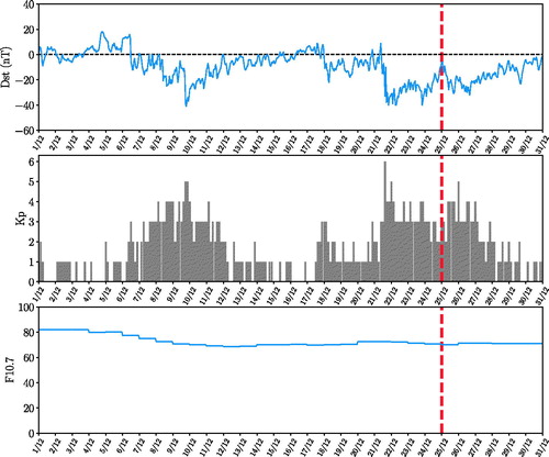
Geomagnetic and solar conditions can produce anomalies in the ionosphere (e.g. Jin et al. 2017). Thus, two important geomagnetic indices, Dst and Kp, were observed for the month of December 2016 (Figure 2). The Dst and Kp indices were downloaded from the World Data Center for Geomagnetism in Kyoto (http://wdc.kugi.kyoto-u.ac.jp/wdc/Sec3.html) and the German Research Center for Geosciences (https://www.gfz-potsdam.de/en/kp-index/), respectively. By looking at Figure 2, it can be easily observed that there is noticeably a period of days, December 12–20, 2016, in which the geomagnetic activity remained very quiet (Dst ≥ −20 nT and Kp ≤3). For the period between December 21 and 25, Kp >3 and Dst < −20 nT; hence, there were some weak geomagnetic storms for these days. Similarly, another period where weak storms can be identified is December 8–11, 2016 (Kp >3 and Dst < −20 nT). Additionally, Figure 2 also shows the solar radio flux at 10.7cm (F10.7 index). This index is a good indicator of solar activity and it can be seen that it remained stable during the month of December 2016, which points to low solar activity. Data for the F10.7 index was retrieved as daily averages from the OMNI database (https://omniweb.gsfc.nasa.gov/form/dx1.html).

Figure 2. Dst, Kp and F10.7 indices during the month of December, 2016. The vertical red dashed line points to the day that the earthquake happened.

4. Results and discussion

For the period of days: December 8–11 and December 12–20, 2016, where there was significant geomagnetic activity, the ΔVTEC maps were not further analyzed. Any ionospheric anomaly identification within these two windows of days are influenced by weak geomagnetic storms.

In order to define a boundary where to observe precursors of the Christmas earthquake, the radius of the earthquake preparation zone was calculated using the Dobrovolsky equation: R = 10^0.43M, where R is the radius given in kilometers and M is the earthquake’s magnitude (Dobrovolsky et al. 1979). For the Chiloé earthquake R is ∼1853 km.

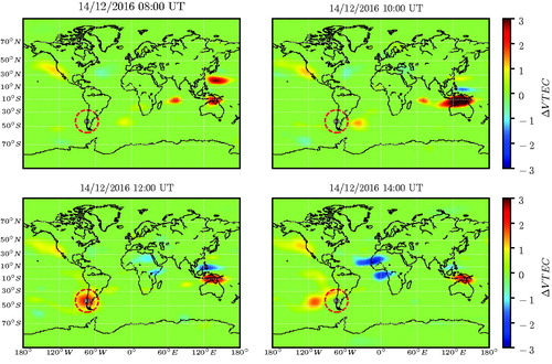
In Figure 3 it can be seen that at ∼10:00 UT (05:00 LT), a positive ionospheric anomaly appears to the west of the earthquake preparation zone. This disturbance at this time has an amplitude of ΔVTEC of 1.40 TECU. At 12:00 UT the anomaly appears right above the epicenter of the seismic event and strikingly covering the whole preparation region. The maximum ΔVTEC at 12:00 UT is 2.13 TECU. At 14:00 UT the ionospheric disturbance moved to the west and with a decrement in its VTEC. After this time, it slowly disappeared. Such a westward displacement was observed in other seismo-ionospheric signatures associated to other earthquakes (e.g. Jing et al. 2011; Yao et al. 2012; Guo et al. 2015). In order to give a possible explanation of how this anomaly arises, the model of Pulinets (2009) is put forward. He explains that radon emanation from the Earth’s crust will ionize the air in the lower atmosphere. If the level of ionization is high, then the air conductivity decreases, which will cause the ionospheric potential to increase, and hence, a positive anomaly would be observed. Enhancement of the radon concentration before strong earthquakes have been already observed (e.g. Inan et al. 2008; Riggio and Santulin 2015); thus, this mechanism could account for the positive ionospheric anomaly observed on December 14, 2016. It is worth mentioning that in Figure 3 there are some additional anomalies far away from the earthquake preparation zone. Especially to the north of Australia at low latitudes and which remained in the same position for several hours. Due to their distance from the earthquake these are considered to be unrelated to the seismic event, and thus their analysis do not fall within the scope of this article.

Figure 3. Differential VTEC maps for December 14, 2016. The grey circles indicate the epicenter of the Chiloé earthquake. The dashed red circles define the earthquake preparation region according to the Dobrovolsky equation (Dobrovolsky et al.1979).

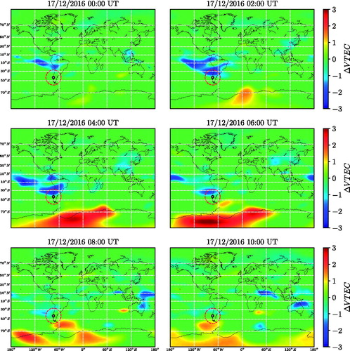
Figure 4 shows the global ΔVTEC for December 17, 2018 between 00:00 and 10:00 UT. It can be observed that at 00:00 UT a negative anomaly is located north of the earthquake preparation zone. This anomaly shows an extension to the west. However, inside the preparation region there is a lack of a disturbance. At 02:00 UT it can be seen that a negative anomaly appears inside the circle defined by the earthquake preparation radius (R), north from the epicenter. The minimum ΔVTEC at this time is of −2.67 TECU. The negative anomaly still remains in the same location at 04:00 UT, although at this time the minimum ΔVTEC decreased slightly, to −2.61 TECU. Starting at 06:00 UT the anomaly begins to weaken and moves westward. At 12:00 UT the anomaly has completely faded away. For a negative ionospheric anomaly to arise, the model of Pulinets (2012) could be followed as well. However, in this case, the ionization level due to radon being released from the Earth's crust will be low. This is going to produce light ions and thus, the air conductivity will increase. The increment in air conductivity will cause a decrease of the ionospheric potential and consequently a negative anomaly will be observed. The ionospheric negative disturbance observed in Figure 4 at low latitudes (north of the earthquake preparation zone) and the very large negative ionospheric disturbance over Antarctica due to their distance to the earthquake preparation zone are considered to be unrelated to the seismic event and originated due to some other physical mechanism.

Figure 4. Differential VTEC maps for December 17, 2016. The grey circles indicate the epicenter of the Chiloé earthquake. The dashed red circles define the earthquake preparation region according to the Dobrovolsky equation (Dobrovolsky et al.1979).

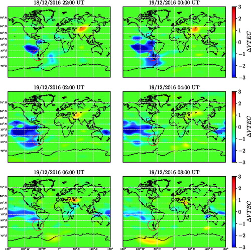
Finally, in Figure 5 between December 18 (22:00 UT) and December 19 (08:00 UT), a second negative anomaly can be observed. Initially, on December 18 at 22:00 UT a negative anomaly northwest from the earthquake preparation zone is clearly visible, while to the east there is also an incoming weak large-scale negative anomaly. On December 19 at 00:00 UT, the weak anomaly moved to the west and at this time, it is right above the earthquake preparation region showing a considerable decrease in VTEC. The minimum ΔVTEC inside the earthquake preparation region for this anomaly is of −2.68 TECU. Two hours after (02:00 UT) the negative anomaly moved to the west and in a similar fashion to the one in Figure 4, this one also started to fade away until ∼08:00 UT, when it disappeared. The mechanism that gave origin to this anomaly could be the same as the one already described for the negative anomaly observed on December 17, 2016 (Figure 4). As observed on December 17, 2016 (Figure 4), there is also on December 18 at 22:00 UT (Figure 5) a negative anomaly northwest to the earthquake preparation zone. This is a low-latitude ionospheric anomaly, and due to the time in which this anomaly was observed, it is very likely that it can be related to a physical mechanism like the fountain effect, which is the main generator of the Equatorial Ionization Anomaly. Hence, it can be suggested that the negative anomaly observed between December 18 (22:00 UT) and December 19 (08:00 UT), 2016 is associated to the earthquake but also has a contribution from the fountain effect, which could explain the extensions seen outside the boundaries of the earthquake preparation region.

Figure 5. Differential VTEC maps for December 18 and 19, 2016. The grey circles indicate the epicenter of the Chiloé earhquake. The dashed red circles define the earthquake preparation region according to the Dobrovolsky equation (Dobrovolsky et al.1979).

Due to the window of quiet geomagnetic activity (Dst ≥ −20 nT and Kp ≤3) between December 12 and 20, 2016, the low solar activity and also due to the fact that the observed disturbances are localized, it is very likely that the three ionospheric anomalies discussed here are associated to the earthquake preparation.

5. Conclusions

Global ionospheric maps from CODE served to analyze ionospheric disturbances prior to the 2016 December earthquake of Mw 7.6 in Chile. This seismic event is product of the subducting Nazca plate. By producing global two-dimensional ΔVTEC maps following a well-known statistical method, it was possible to identify three ionospheric disturbances that happened before the incident. On December 14, 2016, 11 days before the seismic event, a positive ionospheric anomaly was detected. This anomaly only lasted for a few hours and was well-localized, moving westwards during its duration. On the other hand, 8, 7 and 6 days (December 17, 18, and 19, 2016) prior to the earthquake, two negative ionospheric anomalies were also observed. On December 17, 2016 there were observed as well large-structure ionospheric anomalies well outside the earthquake preparation zone (north of it and over Antarctica). Due to their distance from the preparation region they are not considered to be related to the seismic event. On the very late hours of December 18 and early hours of December 19, 2016, a large negative ionospheric structure was also observed at low latitudes. It is suggested that this anomaly north to the preparation region is originated due to the fountain effect from the EIA. Moreover, it is possible that the fountain effect contributes to the generation of the negative anomaly that falls inside the earthquake preparation region between December 18 and December 19, 2016.

All three anomalies were seen to fall inside the earthquake preparation region. Because during the days in which all three anomalies were observed, the geomagnetic and solar conditions were rather quiet and also the anomalies were localized, it could be suggested that they are seismo-ionospheric signatures to the Chiloé earthquake. Furthermore, the origin for these three anomalies could be attributed to the air ionization coming from the Earth's crust.

Data availability statement

The data that support the findings of this study are openly available at ftp://ftp.aiub.unibe.ch/CODE/

Acknowledgments

The author is grateful to the Center for Orbit Determination in Europe for making IONEX files available to the community.

Disclosure statement

No potential conflict of interest was reported by the author.

References

- Alcay S. 2016. Analysis of ionospheric TEC variations response to the Mw 7.2 VAN-earthquake. Acta Geodynam Geomate. 13:257–262.
- Appleton EV. 1946. Two anomalies in the ionosphere. Nature. 157(3995):691.
- Daneshvar MRM, Freund FT. 2017. Remote sensing of atmospheric and ionospheric signals prior to the Mw 8.3 Illapel Earthquake, Chile 2015. New York: Springer International Publishing; p. 157–191.
- Dobrovolsky IP, Zubkov SI, Miachkin VI. 1979. Estimation of the size of earthquake preparation zones. Pure Appl Geophys. 117(5):1025–1044.
- Guo J, Li W, Yu H, Liu Z, Zhao C, Kong Q. 2015. Impending ionospheric anomaly preceding the Iquique Mw 8.2 earthquake in Chile on 2014 April 1. Geophys J Int. 203(3):1461–1470.
- Hasbi AM, Mohd Ali MA, Misran N. 2011. Ionospheric variations before some large earth-quakes over Sumatra. Nat Hazards Earth Syst Sci. 11(2):597–611.
- Inan S, Akgül T, Seyis C, Saatçilar R, Baykut S, Ergintav S, Baş M. 2008. Geochemical monitoring in the Marmara region (NW turkey): a search for precursors of seismic activity. J Geophys Res: Solid Earth. 113(B3):B03401
- Jin S, Jin R, Kutoglu H. 2017. Positive and negative ionospheric responses to the March 2015 geomagnetic storm from BDS observations. J Geodesy. 91:613–626.
- Jing X, Yiyan Z, Wu Yun W. 2011. Ionospheric VTEC anomalies before Ms7.1 Yushu earthquake. Geodesy Geodynam. 2(2):48–52.
- Lange D, Ruiz J, Carrasco S, Manrquez P. 2018. The Chiloé Mw 7.6 earthquake of 2016 December 25 in Southern Chile and its relation to the Mw 9.5 1960 Valdivia earthquake. Geophys J Int. 213(1):210–221.
- Li J, You X, Zhang R, Meng G, Shi H, Han Y. 2015. Ionospheric total electron content dis-turbance associated with May 12, 2008, Wenchuan Earthquake. Geodesy Geodyn. 6: 126–134.
- Liu JY, Chuo YJ, Shan SJ, Tsai YB, Chen YI, Pulinets SA, Yu SB. 2004. Pre-earthquake iono-spheric anomalies registered by continuous GPS TEC measurements. Ann Geophys. 22(5):1585–1593.
- Lomnitz C. 2004. Major earthquakes of Chile: a historical survey, 1535–1960. Seismol Res Lett. 75(3):368.
- Mubarak WA, Abdullah M, Misran N. 2009. Ionospheric TEC response over Simeulue earth-quake of 28 March 2005. In 2009 International Conference on Space Science and Communication; p. 175–178.
- Oikonomou C, Haralambous H, Muslim B. 2017. Investigation of ionospheric precursors related to deep and intermediate earthquakes based on spectral and statistical analysis. Adv Space Res. 59(2):587–602.
- Pulinets SA. 2009. Physical mechanism of the vertical electric field generation over active tectonic faults. Adv Space Res. 44(6):767–773.
- Pulinets SA. 2012. Low-latitude atmosphere-ionosphere effects initiated by strong earth-quakes preparation process. Int J Geophys. 2012:1.
- Pulinets SA, Legen’ka AD. 2002. Dynamics of the near-equatorial ionosphere prior to strong earthquakes. Geomagn Aeronomy. 42:227–232.
- Pundhir D, Singh B, Singh OP, Gupta SK. 2015. Study of ionospheric precursors related to an earthquake (M = 7.8) of 16 April, 2013 using GPS-TEC measurements: case study. J Geogr Nat Dis. 5(1):1–3.
- Reddy CD, Shrivastava MN, Seemala GK, González G, Baez JC. 2016. Ionospheric plasma response to Mw 8.3 Chile Illapel earthquake on september 16, 2015. Pure Appl Geo-Phys. 173(5):1451–1461.
- Ren Z, Yuan Y, Wang P, Fan T, Wang J, Hou J. 2017. The september 16, 2015 Mw 8.3 Illapel, Chile earthquake: characteristics of tsunami wave from near-field to far-field. Acta Oceanol Sin. 36(5):73–82.
- Riggio A, Santulin M. 2012. Earthquake forecasting: a review of radon as seismic precursor. Bollettino Geofisica Teorica Appl. 5(1):1–114.
- Ruiz R, Madariaga R. 2018. Historical and recent large megathrust earthquakes in Chile. Tectonophysics. 733:37–56.
- Ruiz S, Moreno M, Melnick D, Campo F, Poli P, Baez JC, Leyton F, Madariaga R. 2017. Reawakening of large earthquakes in south central Chile: the 2016 Mw 7.6 chilo event. Geophys Res Lett. 44(13):6633–6640.
- Schaer S, Gurtner W, Feltens J. 1998. IONEX: the ionosphere map exchange format version. 1:233–247.
- Thorne L, Yue H, Brodsky EE, Chao A. 2014. The 1 April 2014 Iquique, Chile, Mw 8.1 earthquake rupture sequence. Geophys Res Lett. 41(11):3818–3825.
- Ulukavak M, Yalcinkaya M. 2017. Precursor analysis of ionospheric GPS-TEC variations before the 2010 M7.2 Baja California earthquake. Geomatics. Nat Hazards Risk. 8(2):295–308.
- Wang L, Jinyun G, Xuemin Y, Honguan Y. 2014. Analysis of ionospheric anomaly preceding the Mw 7.3 Yutian earthquake. Geodesy Geodyn. 5(2):54–60.
- Xinzhi W, Junhui J, Dongjie Y, Fuyang K. 2014. Analysis of ionospheric VTEC disturbances before and after the Yutian Ms 7.3 earthquake in the Xinjiang Uygur Autonomous Region. Geodesy Geodyn. 57:8–15.
- Yao YB, Chen P, Wu H, Zhang S, Peng WF. 2012. Analysis of ionospheric anomalies before the 2011 Mw 9.0 Japan earthquake. Chin Sci Bull. 57(5):500–510.
- Zakharenkova IE, Krankowski A, Shagimuratov II. 2006. Modification of the low-latitude ionosphere before the 26 December 2004 Indonesian earthquake. Nat Hazards Earth Syst Sci. 6(5):817–823.
- Zakharenkova IE, Shagimuratov II, Tepenitzina NY, Krankowski A. 2008. Anomalous modification of the ionospheric total electron content prior to the 26 september 2005 Peru earthquake. J Atmos Sol-Terr Phys. 70(15):1919–1928.
- Zhao B, Wang M, Yu T, Wan W, Lei J, Liu L, Ning B. 2008. Is an unusual large enhancement of ionospheric electron density linked with the 2008 great Wenchuan earthquake? J Geophys Res-Space Phys. 113:A11304
- Zhou Y, Wu Y, Qiao X, Zhang X. 2009. Ionospheric anomalies detected by ground-based GPS before the Mw 7.9 Wenchuan earthquake of May 12, 2008, China. J Atmos Solar-Terr Phys. 71(8):959–966.
- Zhu F, Wu Y, Lin J, Zhou Y. 2010. Temporal and spatial characteristics of VTEC anomalies before Wenchuan Ms 8.0 earthquake. Geodesy Geodyn. 1:23–28.
- Zhu F, Zhou Y, Wu Y. 2013. Anomalous variation in GPS TEC prior to the 11 April 2012 Sumatra earthquake. Astrophys Space Sci. 345(2):231–237.
- Zou Y, Zhao T, 2010. Ionospheric anomalies detected by GPS-TEC measurements during the 15 august 2007 Peru earthquake. In: 2010 International Conference on Microwave and Millimeter Wave Technology; p. 1216–1219.